R E S E A R C H
Open Access
MEA: an energy efficient algorithm for dense
sector-based wireless sensor networks
Mohsen Nickray
1, Ali Afzali-Kusha
1*and Riku Jäntti
2Abstract
In this article, first the energy efficiency of sector-shaped wireless sensor networks is analytically investigated. Based on this study, it is shown that the efficiency of existing data propagation algorithms which consider equal ring width is not optimal and may be improved further. Then, we introduce an energy efficient algorithm for these networks which is called minimum energy algorithm (MEA). The detailed analysis verifies that the proposed algorithm has the minimum energy consumption. Although the main emphasis of the proposed technique is on minimizing the energy, it somehow balances the energy consumption in the sector-shaped network as well. In addition, it is shown that the proposed idea can be applied to all existing energy balancing algorithms. The efficacy of the proposed algorithm is studied for networks with different sizes and node densities. The results show that, for example, for a network with a radius of 440 m and four rings when the MEA algorithm is combined with an efficient full power control algorithm (based on equal ring width), the energy conservation increases 50% more. Finally, the results show that the energy conservation of the proposed algorithm increases with the network size.
Keywords:wireless sensor network, energy efficiency, energy balancing, power control
1. Introduction
Recent advances in wireless and electronic technologies have led to the emergence of wireless sensor networks (WSN) with large-scale nodes. They are used in a wide spectrum of applications from industrial and military applications to health and environmental monitoring. In this kind of networks, different small size sensor types are deployed in the area to monitor, e.g., temperature, motion, noise, and seismic activities. A good survey of WSNs is presented in [1,2]. The sensors are wireless nodes which transmit the collected data (hop-by-hop) to a central station called base station orsink node. Due to critical limitations of the node energy resources (e.g., battery), the nodes should minimize the energy con-sumption during their computation and communication. Therefore, low-power algorithms for WSNs are of prime interest. Among different WSN types, sector-shaped networks, where all the nodes send their data to a single base station, have various applications such as monitor-ing, data gathermonitor-ing, and surveillance [3-5]. In this type
of network, if hop-by-hop transmission is used, in addi-tion to the energy efficiency, the energy consumpaddi-tion balance throughout the network (energy balancing pro-blem) will be another noteworthy issue. In this kind of transmission, nodes which are away from the sink node, communicate to sink node via nodes which are near sink node. Thus, the sensor nodes near the sink node will run out of energy leading to the collapse of the entire network, while the nodes far from the base sta-tion may have a considerable amount of energy. The energy balancing problem for a sector-shaped network has been investigated in several works (e.g.,[3-5]). Authors in [5] proved that in a sector-shaped WSN, in order to minimize the total amount of energy consumed on routing, all the rings must have the same width. Then, to solve the energy balancing problem, they selected proper sizes of rings around the sink by assum-ing adjustable transmission radii for sensors. In [4], to achieve a nearly balanced energy depletion, a non-uni-form node distribution strategy was presented. The authors also proposed q-Switch Routing which was a distributed shortest path routing algorithm tailored for the proposed non-uniform node distribution strategy.
* Correspondence: [email protected]
1Nanoelectronic Center of Excellence, School of Electrical and Computer Engineering, College of Engineering, University of Tehran, P.O. Box 14395-515, Tehran, Iran
Full list of author information is available at the end of the article
In this article, we propose an energy-efficient algo-rithm for sector-shaped WSNs called minimum energy algorithm (MEA). The reduction of the energy sumption in the proposed algorithm is achieved by con-sidering rings with unequal widths and invoking power control algorithms within each ring. These two mea-sures not only reduce the energy consumption, but also help to balance the energy consumption throughout the network. The techniques proposed in this algorithm may be combined with other methods proposed to deal with the energy balancing problem for reducing their energy consumptions further. The rest of the article is organized as follows. In Section 2, we briefly review the related works while Section 3 describes the network model and some preliminary definitions. In Section 4, we present the proposed MEA algorithm with a detailed analysis. The results are discussed in Section 5. We dis-cuss the energy balancing in Section 6 and, finally, the paper is concluded in Section 7.
2. Related studies
In this section, we briefly review the previous studies which may be classifiedinto two categories, namely, minimizing energy consumption and the energy balan-cing problem.
2.1. Algorithms related to minimizing energy consumption
Many energy-saving techniques for wireless communica-tion systems(including WSNs) have been proposed (see, e.g.,[5-9]). Among them, transmission range adjustment or power control is one of the most important energy-saving approaches which have been the focus of many studies (see, e.g.,[7-9]). The proposed power control algorithms are either proposed and used in general topology control applications [7] or special applications, such as routing or data gathering in WSNs [8,9]. In [7], the algorithm was proposed for general many-to-many wireless ad-hoc networks (and not sector-shaped WSNs). The power control approach in [8] minimized the total consumed energy for reaching the destination by lowering the energy consumed per unit flow of pack-ets. In this article, static ad-hoc networks or networks with very slowly changing topology (which has enough time for optimally balancing the traffic in the periods between successive topology changes) were considered. In this study, also the topology of the network was assumed static (or very slowly changing) but for a sec-tor-shaped network. In [9], another power control for general wireless ad-hoc networks which considered link error rates on the effective energy consumption was proposed. Compared to the studies [7-9], our approach focuses on reducing the energy consumption of a sec-tor-shaped many-to-one network and introduces the
most energy-efficient algorithm using the power control algorithm. Olariu and Stojmenovic [5] presented some design guidelines for minimizing the energy consump-tion of a sector-shaped network. They considered uni-formly distributed sensors, each sending roughly the same number of reports toward the sink. This study was not based on a power control mechanism. In [6], the authors considered a sector-shaped many-to-one net-work with a uniform node distribution and constant data reporting rate. The algorithm presented in this study, which was based on a power control scheme, minimizes the energy consumption when the same width was used for all the rings and the transmission ranges of the nodes were adjustable. They also proposed a technique for eliminating the energy balancing pro-blem (see Section 2.2). To the best of the authors’ knowledge, the algorithm discussed in [6] leads to the lowest energy consumption for the sector-based net-works when compared to other algorithms. The main difference between our algorithm with that of [6] is the definition of new borders which are called hop borders, in addition to traditional network borders defined in [6]. Based on these hop borders, the number of relay hops are optimized minimizing the energy consumption. To assess the efficiency of our algorithm, we have compared the results of our algorithm with those of [6] as basic algorithm (BA).
2.2 Algorithms related to energy balancing problem The problem of overusing the nodes near the sink node has been studied with different terminologies. In [10], the problem has been investigated as an energy hole problem while the authors in [3] call this a doughnut problem. In [3,11], the problem is studied under the subject of balancing the lifetime and bottleneck pro-blem, respectively. Although the algorithm proposed in this article intends to minimize the energy consumption, it somehow lessens the energy balancing problem and may be combined with the existing algorithms dealing with the problem. Next, we review some of works related to the energy balancing problem which may be categorized into four approaches, namely, power control, mobility, multiple battery level, and non-uniform placement.
2.2.1. Power control approaches
cheap one-hop transmission and direct transmission which is more expensive but bypass the sensors near the sink node. To remedy the energy imbalance pro-blem, the technique in [5] assumed that the transmis-sion range of sensors are adjustable and attempt to balance the energy consumption among sensors by selecting proper sizes of rings around the sink node. The transmission radius of a given sensor is adjusted based on the width of the ring containing it. It is shown that the width of the rings in an energy-balanced sensor network should be increased with the distance to the sink. Finally, to solve the problem, Li and Mohapatra [13] proposed an algorithm based on the transmission range. Their analysis showed that decreasing the transmission range of the nodes as we move toward the BS decreases maximizes the lifetime of the nodes. Based on this analysis they calculated the exact transmission range of the nodes.
2.2.2. Mobility approaches
To solve the energy hole problem, the use of mobile sink, relay, and sensor nodes is suggested in [14-16]. The solution of using a mobile sink node which makes the nodes close to the sink node change over time is suggested in [14]. They optimize the proposed approach by considering both sink mobility and multi-hop routing algorithms simultaneously. Using a detailed analytical model, they showed that the algorithm provided five times network lifetime improvement. In [15], authors investigated the impact of relay and sink node mobility. They found that using the mobile sink node maximized the lifetime. Also, it was shown that for a very dense network, the lifetime may be improved four times if a static sink node and mobile relay nodes are used. Finally, the use of mobile sensor nodes in a hexagon mechanism (dividing the network area into six-side shapes) was proposed in [16].
2.2.3. Multiple battery level approach
Authors of [3,17,18] present a scheme to distribute the total energy budget in multiple battery levels where the closer a node is to the BS, the larger share of the total initial energy (battery) is allocated to this node. Under a total energy budget, they have shown a method to com-pute the optimal battery levels and number of nodes for each battery level. With this strategy, they have shown that lifetime of the network can be significantly improved, even if a small number of battery levels is used.
2.2.4. Nonuniform placement approach
In [11], in order to solve the doughnut problem, the use of higher node density close to the base station is sug-gested. They proposed that if the density of sensor nodes increased as we move toward to the base station, the doughnut effect could be minimized. They deter-mined the density of the sensor nodes at a particular
distance from the BS for avoiding the bottleneck phe-nomenon around it. In [5], for a sector-shaped network with a uniform node distribution and data reporting rate, it is proved that the hole problem for 7 >a(path loss factor) > 2 is preventable while fora = 2, uneven energy depletion is unavoidable regardless of the routing strategy. Then, the authors of [5,6] showed that the energy consumption for the data transmissions can be balanced when the node density of the ith ring is pro-portional to k - 1-i where k is the optimal number of coronas. In [4], the authors, first, analytically proved that a fully balanced energy depletion among all the nodes was impossible. Then, they proposed a node dis-tribution strategy for achieving suboptimal balanced energy depletion. The strategy was based on growing the number of nodes with a geometric proportion from outer (peripheral) to the inner. In this technique, the ratio between the node densities of the two adjacent coronas of (i+ 1)th andith is equal to (2i- 1)/q(2i+ 1), whereq is the geometric proportion mentioned above. A routing algorithm was also proposed for this non-uni-form node distribution strategy.
3. Preliminaries
In this section, we state some definitions and assump-tions used in this study. Then, the proposed algorithm is described and analyzed. Some of the main assump-tions in this study are
- The WSN network is a very dense composed of a large number of sensors.
- Nodes are uniformly distributed. Thus, the node density is obtained from r = n/A where n is the number of nodes andAis the network area.
- Sensors have an adjustable transmission range. - Each node continuously generates a constant bit rate ofLbits per time periodand sends data to the sink node through a multi-hop route.
- The events which should be reported to the sink node are happening uniformly too.
from the perspective of lifetime properties(N network cells) and is divided intokcells from the perspective of node density (knode cells). It should be noted that the network (node) cells have the same area and Nand k
may be different. Figure 1 shows ψ(π/6,R,4,16) which contains 4 network cells (Figure 1a) and 16 node cells (Figure 1b). If the number of node cells is assumed equal with the number of sensor nodes, then according to the assumption of the uniform placement of the nodes, for a very dense network, we can assume one node in each node cell. Now, we present some of the definitions used in our analysis:
Definition 1. Network annuluses and network cells The sector area is divided into ring slices with the same ring width which are called network annulus. The net-work annuluses in this study have the same meaning of corona in [4,5] or ring in [3]. The areas of these net-work annuluses are not equal. Each netnet-work annulus may be divided into network cells with equal areas. We will prove that each the annulusi may be divided into 2i- 1 cells with an equal area of. For example, Figure 1a shows a network with two annuluses which annulus 1 contains one cell and annulus 2 contains three cells. The borders between annuluses are called network borders.
Definition 2. Node annuluses and node cells
For the sake of analysis, we assume another ring-based division similar to Definition 1. The only obvious differ-ence is that the number of node annuluses depends on the number of nodes. For example, Figure 1b shows the same network area as that of Figure 1 abut with node annuluses and node cells. The parameterk is assumed to be equal to the number of nodes disseminated through the area.
Note that when we use annulus or cell without the word of network or node, we mean network annulus or network cell.
Definition 3.i-hop network
i-hop network is a network where the maximum num-ber of hops for the transmission is iprovided that the numbers of transmission hops be optimum (e.g., iis 4 in the network shown in Figure 2.)
Definition 4. Lifetime of network (LTψ)
We assume that a network will be alive until all the nodes in one of the network cells are depleted.
Definition 5. Critical cell
The first network cell whose all nodes go out of energy in the whole network area is called critical cell. And always the lifetime of a network is set by the lifetime of its critical cell (LTψ= LTcritical cell). In our sector-based network, the cell in annulus 1 would be the critical cell because not only it should send all the events in its sen-sing area but also should relay the data of all the upper cells to the sink node. Therefore, one may write
LTψ= LTannulus 1 (1)
Definition 6. Networkperiod(Tψ)
It is the time interval in which all the nodes(sequen-tially) in the network cell sense an event and report it to the next hop. Based on the assumption of the uniform distribution for the events, the energy consumption dur-ing this period could be a very good parameter for com-paring the network lifetime (see Definition 7.)
Definition 7. Period energy consumption (EPψ)
Let us assume that we have the network ψwith the per-iod of Tψ. The energy dissipated in the networkψ dur-ing Tψis called the Period energy consumption.
Note that Definitions 6 and 7 for the network period and the period energy consumption may be used for the network annuluses too, with the Tannulus, iandE
p annulus,i,
respectively.
Figure 1Network areaψ(π/6,R,4,16) (a)The network with 4 network cell.(b)The same network which is divided into 16 node cells.
According to the above definitions, we can declare LTψmore precisely
LTψ= LTcritical cell=
sum of initial energy of all nodes in critical cell EP
critcal cell
(2)
3.1. Energy model
Note that since in this study we focus on multi-hop sen-sor networks, we should also pay attention to the receive energies in the energy model. It originates from the fact for small size networks, due to extremely small transmission distances, the power consumed while receiving data can often be greater than the power con-sumed while transmitting packets [18]. Also, the over-head energy consumption for the node wake up cannot be assumed insignificant. In this article, we adopt the first-order radio model described using [19] as
Etxpacket(L,d) =Ew+L.Etxe +L.Er.dα (3)
Erxpacket(L, d) = L×Erxe (4)
The model express the network transmit and receive energy consumption for a linear communication as a function of path loss factor (a)distance between trans-mitter and receiver (d), the packet size (L), fixed energy overhead for the radio start up (Ew), electronic circuitry (Ee), and energy consumed by the power amplifierEr. We should notify that in these formula we assume EeTx =EeRx=Ee.
The parameter a can have a value between 2 and 6 [19]. For short distances, its value is assumed to be 2 (see, e.g., [20]). In this study, we have considered dense WSNs where the network nodes are very close to each other, and hence, we usedaas 2.
4. Minimum energy algorithm
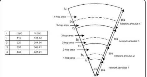
As mentioned previously, the authors of [4] show that the total energy spent per routing path is minimized when the network is set up with equal annulus width. Based on this, the sector-shaped algorithms presented in [3-5] used annuluses with the same width. Figure 2 shows the sector area for a 4-hop network whereb1 -b3 and r1 - r3 define the hop and network borders, respectively.
Definition 8. Hop border (bi)
Hop borders are circular borders which are set around the sink node in the sector (see, e.g., Figure 2). When a node is between the borders biand bi+1, it means that the energy consumption for the transmission from the node to the sink node could be minimized if i + 1
transmission hops are used. These borders are obtained from Equation (5).
Definition 9.i- 1-hop area andi-hop area
We will show that the hop borders biare always
posi-tioned inside annulus i (between ri and ri-1 borders). Therefore, bi-1 divides the annulusiarea into two sepa-rate areas. The area which is defined by ri-1<r < bi-1is calledi - 1-hop area whose nodes transmit data usingi
- 1-hop transmission and the area which is defined by
bi-1<r <riis calledi-hop area whose nodes useani-hop transmission to transmit the data to the sink node.
In the existing conventional algorithms for the sector-shaped networks (in this article we call them BA), the nodes use the network borders (in our example,r1tor3) to decide about the optimum number of hops. In the algorithm proposed in this study, these borders have another functionality which is calculating the lifetime. For instance, in Figure 2, all nodes in annulus 1 use a single-hop transmission while the nodes in the annulusi
(2 ≤i ≤4) use ani-hop transmission (all with a trans-mission range ofR/4) to report events to the sink node.
For two reasons the energy consumption of this BA is not optimum (minimum). First, all the nodes in each network annulus are adjusted with the same transmis-sion range (corresponding to the annulus width). The energy consumption in the network would be minimum if the nodes in annulus 1 adjust their transmission range proportional to their distances from the sink node and the nodes in the annulusi (2≤i≤4) adjust their trans-mission range relative to their distances from their next hop in annulus i - 1. Second, transmitting data usingi
hops is not necessarily optimum for all the nodes in the annulusias is assumed in the BA. For some nodes, the optimum number of hops could be i- 1 (see Figure 2). In our proposed algorithm (MEA) to guarantee the minimum energy consumption, we consider these two issues. Next, we discuss three algorithms for hop-by-hop data transmission in WSN. Table 1 presentsthe BA of the data propagation for a sector-shaped network. In a basic sector-shaped algorithm forψ(a, R, N, k) whichbi
<R<bi+1, the area will be divided intoiannuluses with
Table 1 Basic algorithm
Basic algorithm
- Annulus number is set toiwhenbi-1≤R≤bi(bkfork= 1,...,iis obtained from Equation (5))
- For each nodenin annulusj= 1..i,
Transmission is provided by aj-hop transmission. Transmission
range of node is adjusted based onR
the width ofR/i. All the nodes adjust their transmission range to R/i. Table 2 gives the basic power control (BPC) algorithm which is a modified BA equipped with the power control mechanism for all of the nodes. It has two main differences with BA. First, in annulus 1, the nodes will adjust their transmission range based on their individual distances from sink node. Second, the nodes in the annulus i(i≥ 2), select intermediate relay nodes such that the hop distances become the same. Hence, the nodes use the same transmission powers. Finally, Table 3 defines the MEA which is a modified BPC algo-rithm whose nodes use hop borders to decide about the number of hops and regulate distance from next hop. Using an efficient number of hops, MEA minimizes the total energy consumption of the network (EPψ) increas-ing the lifetime of the network. For example, while in MEA, the nodes in the one-hop region of annulus 2 (see Figure 2)transmit data directly to the base station. The same nodes in BA use a two-hop transmission causing some energy dissipation in annulus 1. This feature of MEA leads to lifetime increase of annulus 1 compared to the case of the BA. It should be noted that annulus 1 is the critical annulus.
Next, we show that MEA provides the minimum energy consumption.
Lemma 1: Assume that we have a large-scale sensor
network whose nodes use a multi-hop transmission to communicate with the sink node, the border for thei -hop, denoted bybi, is obtained from
bi=
mined as the point where ani-hop transmission con-sumes more energy than ani+ 1-hop transmission (E
i-hop> Ei+1-hop). Using the energy model presented in the previous section, one may write the energy consumption fori-hop andi+ 1-hop communications, respectively, as
Ei−hop= iEw+ i×L×Ee+ (i−1)×L×Ee+ i×L×Er×
Therefore, for Ei-hop(d) > Ei+1-hop(d), we should have
d>
i(i + 1)(Ew+ 2LEe)
LEr
(8)
It means for a node with distance greater thandfrom the sink node, ani+ 1-hop communication outperforms an i-hop one. This determines the border bi equal to
i(i + 1)(Ew+ 2LEe)
LEr
.
Lemma 2: In ani-hop sector-shaped network, always
we have (a)bj≥rjforj= 1...iand (b)rj+1≥bjfor j= 1...i
- 1.
Proof:(a) For ani-hop network, we havebi>R≥bi-1
where the maximum value forRis bi. Based on Equation (5), we may write
Considering bj=
minimum value forRis bi-1. Based on Equation (5) we have
Considering bj=
Lemma 3:In ani-hop communication, equal hop
dis-tances among the relay nodes lead to the minimum energy consumption (maximum network lifetime). The minimum energy consumption for linear networks is proved in [21,22].
Theorem 1: MEA algorithm is the minimum
algorithm.
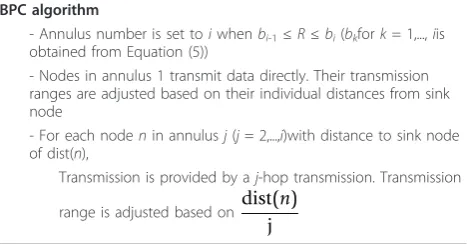
Table 2 BPC algorithm
BPC algorithm
- Annulus number is set toiwhenbi-1≤R≤bi(bkfork= 1,...,iis obtained from Equation (5))
- Nodes in annulus 1 transmit data directly. Their transmission ranges are adjusted based on their individual distances from sink node
- For each nodenin annulusj(j= 2,...,i)with distance to sink node of dist(n),
Transmission is provided by aj-hop transmission. Transmission
range is adjusted based ondist(n)
The communication energy consumption of the pro-posed algorithm is minimum if all the communications in network are performed using a data propagation technique with the minimum energy consumption. In other words, the algorithm will be minimum if the energy consumptions of all annuluses are minimum. Now, we study the proposed algorithm to see if it is an optimum algorithm. Let us assume that we have a net-work withiannuluses. Based on Lemma 2, alwaysb1 ≥ r1. Then, for the nodes in annulus1, a single-hop trans-mission guarantees the minimum energy consumption. The transmission ranges of these nodes are adjusted by their distances from the sink node. Thus, the algorithm provides the minimum energy consumption for the nodes in annulus1.
For annuluses 2 toi, based on Lemma 2, we haverj≤
bj ≤ rj+1 for j = 1,...,i - 1. Based on Definition 9, bj
divides the area of the annulusjinto twoj- 1-hop and
j-hop areas. Let us denote the distance of any arbitrary nodeq(p) in thej-hop (j- 1-hop) area byrj-hop,q(rj-1-hop,
p). For the nodes in the j-hop andj - 1-hop areas, we
will have rj+1 >r(j)-hop,q ≥ bj and bj >r(j - 1)-hop,p ≥ rj
which meansjandj- 1 are the optimum hop numbers for the nodes in j-hop andj- 1-hop areas, respectively. Based on Lemma 3, the energy consumption will be minimized if the distances between the intermediate
hops are equal to
r(j−1)−hop, p
j−1 and
r(j)−hop, p
j ,
respectively.□
Next, to evaluate the proposed algorithm more accu-rately, we analyze the period energy consumption of MEA and BPC algorithms. Assume that we have a sec-tor-shaped network containing knode cells. To be able to divide the sector area into k cells, k should be a square number. We divide the whole sector area into
√
k annuluses with the width of √R
k and 2i- 1 cells in the annulus i. If the number of the node areas is assumed equal with the number of the sensor nodes, then according to the assumption of uniform placement of the nodes, for a very dense network, we can expect
that have one node in each node cell. The number of node cells and distance of each node from the sink node is defined using Lemma 4.
Lemma 4:For the network ψ(a, R, N, k), (a) the
dis-tance of a node in the node annulus i from the sink
node is √iR
k and (b) the node annulusihas 2i- 1 node cell.
Proof:(a) For the network ψwhich containsknodes,
we will have an area withk equal node cells. The sec-tor-shaped area may be divided into √k node annuluses
with a radius of √R
k whichwe can number them from 1 to #√k. The maximum distances from the sink node
for a node in annulus1, 2, and annulus i are √R k,
2R
√
k,
and √iR
k, respectively. The maximum distance for the
nodes in the last annulus (annulus √k) is
√
k×√R k = R.
(b) In the analytic model, we assume that we havek
node cells where each cell contains one node. The area of annulus1 with only one cell is assumed as the unit cell and is given by
Area of annulus1 = Area of unit cell = α 2×
R
√
k 2
(11)
Based on this, the area of annulusiis given by
Area of annulus i =α 2
iR
√
k
2
−α
2
(i−1)R
√
k
2
=α 2
R
√
k
2
(2i−1)
= (2i−1)×area of unit cell
(12)
Therefore, we can conclude the annulusi has (2i- 1) equal node cells.□
In the BA algorithm, the transmission range of all the nodes in annulusi is adjusted toR/i which is equal to the annulus width. Then, traffic of data transmissions of the nodes in annulusiis distributed on the whole nodes
Table 3 Minimum energy algorithm
Minimum energy algorithm
- Annulus number is set toiwhenbi-1≤R≤bi(bkfork= 1,...,iis obtained from Equation (5))
- Nodes in annulus 1 transmit data directly. Their transmission ranges are adjusted based on their individual distances from sink node - For each nodenin annulusj(j= 2, ...,i) with distance to sink node of dist(n)
if ri-1≤dist(n) < bi
Transmission is provided byj- 1 hop communication. Transmission range is adjusted based ondist(n)
(j−1)
else
Transmission is provided byjhop communication. Transmission range is adjusted based ondist(n)
of the annulusi- 1. The traffic distribution in the MEA algorithm is different from BA owing to different beha-viors of nodes ini - 1-hop andi-hop areas in selecting the next hop. As is shown in Lemmas 5 and 6, the traf-fic of the nodes ini - 1-hop area andi-hop area of the annulusiis distributed ini- 1-hop area and i-hop area of the annulusi- 1, respectively.
Lemma 5:The traffic of all the nodes in thei-hop area
of annulusiis relayed by the nodes in thei-hop area of annuluses 1 toi- 1.
Proof:For a node at the distance rsuch thatbj<r ≤rj
+1, the optimum number of hops is j+ 1. Also, using Lemma 3, the best positions for the intermediate hops, denoted by disti (the distance of theith hop from sink
node) is obtained from
disti=
(j + 1−i)
j + 1 ×r i = 1. . .j (13)
To prove the lemma, we should show that for all the values of ibetween 1 and j, rj+1-i≥ disti> bj-i. First, we show the validity of disti> bj-i. Note that the minimum value of r will be bj, and hence, we may write
distmini = (j + 1−i)
j + 1 ×bj i = 1. . .j (14)
Plugging the minimum value for the intermediate hop positions and Equation (5) into the inequality of distmini >bj−i, we obtain
This equality is valid for i > 0 which is always true. Since distmini >bj−i, we can have disti> bj-i.
Next, the validity of rj+1-i≥distiis shown. We have
disti=j + 1−i
Lemma 6: The traffic of data transmission of all the
nodes ini - 1-hop area of the annulus i is relayed by nodes ini- 1-hop areas of annuluses 1 to i- 1.
Proof:For a node at distance r such that bj <r ≤rj,
the optimum number of hops isj. Also, using Lemma 3, the best positions for the intermediate hops, denoted by disti (the distance of the ith hop from sink node) is
obtained from
disti=
j−i
j ×r i = 1. . .j−1 (18)
To prove the lemma, we should show that for all the values ofibetween1 andj- 1, bj-i≥disti> rj-i. First, we show the validity of bj-i≥ disti. Note that the maximum value ofr will be bj, and hence, we may write
distmaxi = j−i
j ×bj i = 1. . .j (19)
Plugging the maximum value for the positions of the intermediate hops and Equation (5) into the inequality of bj−i≥distmaxi , we obtain
This equality is valid for i > 0 which is always true. Since bj−i≥distmaxi , we can have bj-i≥disti.
Next, the validity of disti> rj-iis shown. We have
disti>rj (22)
Next, based on Lemmas 4, 5, and 6, we analyze the period energy consumption of MEA and BPC algorithms.
Theorem 2: The period energy consumption of MEA
Lry(j) = (
Proof:The network is divided into Nnetwork cells
and √N network annuluses numbered from 1 to √N. From the perspective of node density, the network is divided intoknode cells and √k node annuluses num-bered from 1 to √k. Also, the node annulus numbers
in the network annulus j are numbered from
(j−1).k/N + 1 to j.k/N. The period energy
con-sumption is the sum of the consumed energy in all the annuluses obtained from
The energy consumption of each network annulus based on Equations (3) and (4) is sum of three terms “receive circuit energy”, “transmit circuit energy”, and “transmit radio energy.”For example, for network annu-lus 1, one may write
Epannulus 1(MEA)
We assume that the sensed data per node will be L
bit. The average received/relayed data per node for nodes in annulus 1 is denoted by Lr(1). Based on the network cell number(N) and node cell number(k), the
number of nodes in each network cell is obtained ask/ N. The sum of the receive and transmit circuit energies
for all the nodes in network annulus 1 is k N.L
e, respectively. Thesek/Nnodes are
distributed in k/Nnode cell from node annulus 1 to the
node annulus k/N. Based on Lemma 4 and the
assumption of the uniform distribution, in each annulus, there are 2i- 1 nodes with a distance of ir/√k from the sink node. The total radio energy for all the nodes in
annulus 1 will be
(L + Lr(1)).Er.
The energy consumption of the other annuluses may be calculated by a similar discussion. The only differ-ence is that all the other network annuluses are divided into two i- 1-hop andi-hop areas. It should be noticed that the node annulus which acts as the border between
i - 1-hop area and i-hop area is denoted by Di. While the best situation occurs when biis exactly at the border of two annuluses, in most cases, it occurs inside one of the node annuluses. In these cases, the question is which node annulus should be selected as Di. We can select the annulus which contains bior the lower annu-lus. In our analysis we assume Dias
Di=
Z(j) = (
Based onLemmas5 and 6, we know that the relayed data for the i - 1-hop and i-hop areas is completely separated. Thus, we define two relay parameters for each annulus which are Lr
y(j) for thei - 1-hop area and obtained from the accumulated data of all the i- 1-hop areas of all the upper annuluses. It means that all the data of the i- 1-hop areas are accumulated in thei - 1-hop area of annulus 2 where it is sent to the base sta-tion. Also, Lr
z(j) is the accumulated data of all thei-hop
areas of the upper annuluses. This traffic finally will be relayed to the nodes in annulus1. Then relay data for the nodes in annulus1 will be the summation of all the accumulated data of thei-hop areas of all the annuluses as
Finally, based on Equation(30), the summation of the period energy consumption of all annuluses leads us to total Epψ(MEA).□
Theorem 3. The period energy consumption of BPC
for a network ofψ(a, R, N, k) is given by
Proof:The total energy of the BPC algorithm is
obtained in a method very similar to that of the MEA algorithm (Epψ(MEA)). The only difference is that, in this case, the complication of dividing the annuluses into two i- 1-hop and i-hop areas does not exist, and hence, we do not repeat the proof here. Note that in this case,X(j) and Lrx(j) denote the number of nodes in the annulusjand the average data relayed by the nodes in the annulusj, respectively.□
5. Results and discussion
In this section, we study the results of the energy con-sumptions and lifetimes of the networks when the pro-posed MEA and BPC algorithms are used. In the study, the effect of considering the power control in the BPC algorithm and the impact of hop-borders in MEA algo-rithm are evaluated. All the results are obtained using the parameters given in Table 4. All the results are gen-erated in Matlab 7.3.
Figure 3 compares the total (period) energy consump-tions of the BA and BPC algorithms versus the number of nodes for two networks with R = 350 and 440 m. The networks contain 16 network cells. For example, the figure shows that for a sector-shaped network with
R = 350 m and 1600 nodes, the proposed BPC algo-rithm leads to more than 18% energy preserving when compared to the BA. For a network with R = 440 m, the improvement is more than 23%. Next, in Figure 4, we compare the MEA algorithm with the BPC one to evaluate that efficiency of the idea of separating the
i-hop and i - 1-hop areas. For the sector-shaped net-work with R = 350 m and 1600 nodes, the algorithm MEA shows a 50% energy preserving when compared to the BPC algorithm. In the case of R = 440 m, the improvement of the MEA algorithm over the BPC algo-rithm is not high. Note that BPC itself is already a very
Table 4 Energy parameters used for obtaining the results
power-efficient algorithm when compared to BA. Next, we study the efficiency of the proposed propagation algorithm on the prolonging network lifetimes.
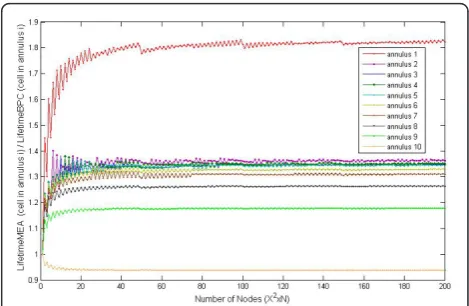
Figure 5 compares the lifetimes of different annuluses versus the number of nodes when the MEA and BPC algorithms were applied to a network with R = 1 km andN= 100. The results show that the MEA algorithm increases the lifetime of all the annuluses except for annulus 10. This is because the transmissions in thei -1-area consume more energy than the nodes with the same position in BPC. The reason is that these nodes in the MEA technique use a 9-hop transmission while in the BPC method a 10-hop transmission is utilized. This degrading factor exists in all the annuluses 2 to 10. In annuluses 2 to 9, energy preserving ofi-hop area com-pensate it but in annulus 10, i-hop area is not large enough to compensate thisi - 1-hop degrading effect. Also, it should be noted that the closer the annulus is to the base station, the higher is the improvement in the annulus lifetime. Based on these results, it may be con-cluded that the proposed MEA algorithm, not only can
lower the energy consumption but also it can alleviate the imbalance problem in sector-shaped networks. To study the scalability of the algorithm, the algorithm was applied to networks with different number of network cells whose lifetimes have been presented in Figure 6. The study included three network configurations with radiuses of 400, 800, and 1300 m which had 16, 64, and 169 network cells, respectively. The results clearly indi-cated that the performance of the MEA increases when the network size.
Figure 7 presents the ratio of lifetimes in the BPC and BA algorithms versus the radius and number of nodes for N = 100. As the results reveal, the lifetime of the BPC algorithm increases with the network size. This was expected based on the fact that, in BA, the trans-mission range of all the nodes in annulus 1 is adjusted based on the radius of annulus 1. For this case, increas-ing the radius makes the energy consumption of annu-lus1 less efficient. Also, the results show that the efficiency of using power control mechanism increases Figure 3Ratio of period energy consumptions of the BA and
BPC algorithms for two cases ofR= 440 m andR= 350 m and
N= 16.
Figure 4Ratio of period energy consumptions of the BPC and
MEA algorithms for two cases ofR= 440 m andR= 350 m
andN= 16.
Figure 5The ratio of lifetimes of annulus 1 to 10 in the MEA
and BPC algorithms forR= 1 km andN= 100.
Figure 6The ratio of lifetimes in the MEA and BPC algorithms
versus number of nodes for networks withN= 16, 64, 169,
as the number of nodes or node density enlarges. Simi-larly, the ratio of lifetimes in the MEA and BPC algo-rithms versus the radius and number of nodesare plotted in Figure 8 for the same configuration as that of Figure 7. The results show that the increase in the radius size decreases the lifetime ratio. This originates from the fact that when the radius size enlarges, Lr
Z(j)
for annulus jincreases enlarging Lr(1) and reducing the efficiency of MEA algorithm. Similar results as those of Figure 8 except forN= 4 are presented in Figure 9. The comparison between Figures 8 and 9 indicates the ratio of lifetime in the MEA and BPC algorithms increases with the network size.
6. Energy consumption balancing
As was discussed before, the main objective and focus of the proposed algorithm is to minimize the energy con-sumption of the network. Since the energy balancing property of sector-shaped networks is very important, in this section, using an example, we show that the MEA algorithm may be combined with any of the balancing algorithms to make them more efficient approaches. In this section, we use the energy balancing technique of [3] which used a power control-based algorithm to bal-ance the energy consumption. In [3], for the nodes in the annulus i, wi% of data is propagated directly to the sink node and (1-wi)%is propagated to the next annulus. The optimum wivalues are selected based on the com-promise between a cheap multi-hop transmission and direct transmission which is more expensive but bypasses the nodes near the sink node. The parameters wiare extracted from [3]
Ep(1)= E
p(2)
3 =
Ep(3)
5 =. . . Ep(i)
2i−1, (41)
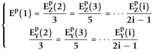
where Ep(i) is the period energy of annulus i. This approach may easily be combined with MEA making it a Balanced-MEA algorithm. Based on Lemmas 5 and 6, in thei- 1-hop andi-hop areas, we have traffics with differ-ent characteristics. Thus, Equation (10)is changed to
⎧ ⎪ ⎪ ⎨ ⎪ ⎪ ⎩
Ep(1) = E
p Z(2)
3 =
EpZ(3)
5 =· · · EpZ(i)
2i−1
EpY(2)
3 =
EpY(3)
5 =· · · EpY(i)
2i−1
(42)
where EpZ(i) and EpY(i) denote the energy consump-tions of the i- 1-hop and i-hop areas of the annulusi, respectively, which were included in the algorithm. Similarly, the MEA algorithm may also be combined Figure 7The ratio of lifetimes in the BPC and BA algorithms
versus radius and number of nodes forN= 100.
Figure 8The ratio of lifetimes in the MEA and BPC algorithms
versus radius and number of nodes forN= 100.
Figure 9The ratio of lifetimes in the MEA and BPC algorithms
with other energy balancing algorithms such as different battery level approaches [3,17] and non-uniform place-ment approaches [4,5], and mobility approaches [14-16]. In both of these techniques, for each of the i - 1-hop and i-hop areas, we have one set of equations. In the former approach, the equations provide the battery level while in the latter case, they present the node density for all the areas.
7. Conclusion
In this article, we proposed an MEA for sector-shaped networks. First, we showed that the (transmission) energy consumption with equal ring width was not opti-mal. Then, we introduced an algorithm which did not assume an equal ring width and showed that the energy efficiency of the network improved further in this case. Second, noting the fact that in the existing algorithms, the transmission power of all the nodes inside a ring was considered equal, we studied the effect of the power control for the nodes of a ring. The study showed that utilizing a power control algorithm for the ring nodes lowers the energy consumption further. To determine the efficiency of the proposed algorithm, we compared two other algorithms, one with power control and one without it. The comparison which was performed for networks with different sizes and node densities showed considerable improvements on the energy consumption and lifetime of the network. In addition, the proposed algorithm alleviated the energy balancing problem of this type of network. Finally, we showed that the MEA algorithm could be combined with other energy balan-cing algorithms making them more efficient.
Acknowledgements
MN and AAK acknowledge the financial support by Iran Telecommunication Research Center (ITRC).
Author details
1Nanoelectronic Center of Excellence, School of Electrical and Computer Engineering, College of Engineering, University of Tehran, P.O. Box 14395-515, Tehran, Iran2Department of Communications and Networking, Aalto University, P.O. Box 13000, FI-00076 Aalto, Finland
Competing interests
The authors declare that they have no competing interests.
Received: 24 April 2011 Accepted: 6 March 2012 Published: 6 March 2012
References
1. IF Akyildiz, W Su, Y Sankarasubramaniam, E Cayirci, Wireless sensor networks: a survey. J Comput Netw.38, 393–422 (2002). doi:10.1016/S1389-1286(01)00302-4
2. IF Akyildiz, W Su, Y Sankarasubramaniam, E Cayirci, A survey on sensor networks. IEEE Commun Mag.40(8):102–114 (2002). doi:10.1109/ MCOM.2002.1024422
3. C Efthymiou, S Nikoletseas, J Rolim, Energy balanced data propagation in wireless sensor networks. Wirel Netw J.12(6):691–707 (2006). doi:10.1007/ s11276-006-6529-y
4. X Wu, G Chen, SK Das, Avoiding energy holes in wireless sensor networks with nonuniform node distribution. IEEE Trans Parallel Distrib Syst.
19(5):710–720 (2008)
5. S Olariu, I Stojmenovic, Design guidelines for maximizing lifetime and avoiding energy holes in sensor networks with uniform distribution and uniform reporting.Proc IEEE INFOCOM, Barcelona, 1–12 (April, 2006) 6. S Olariu, I Stojmenovic, Data-Centric Protocols for Wireless Sensor Networks.
inHandbook of Sensor Networks: Algorithms and Architectures, ed. by Stojmenovic I John Wiley & Sons, New York, 417–456 (2005)
7. N Li, JC Hou, L Sha, Design and analysis of an MST-based topology control algorithm.IEEE INFOCOM, San Francisco, 1702–1712 (March, 2003) 8. JH Chang, L Tassiulas, Energy conserving routing in wireless ad-hoc
networks.IEEE INFOCOM, Tel-Aviv, 22–31 (March, 2000)
9. S Banerjee, A Misra, Minimum energy paths for reliable communication in multi-hop wireless networks.MobiHoc, Maryland, 146–156 (June, 2002) 10. J Li, P Mohapatra, Analytical modeling and mitigation techniques for the
energy hole problems in sensor networks. Pervasive Mob Comput.
3(8):233–254 (2007)
11. K Padmanabh, R Roy, Transmission range and density gradient management to avoid bottleneck around base station in wireless sensor network. Int J Commun Netw Distrib Syst.4(1):121–130 (2010) 12. M Singh, V Prasanna, Energy-optimal and energy-balanced sorting in a
single-hop wireless sensor network. inProc First IEEE International Conference on Pervasive Computing and Comminications, PERCOM, Texas, March 2003
146–156
13. J Li, P Mohapatra, An analytical model for the energy hole problem in many-to-one sensor networks.Proc 62nd IEEE Vehicular Technology Conference, Dallas, 2721–2725 (2005)
14. J Luo, JP Hubaux, Joint mobility and routing for lifetime elongation in wireless sensor networks.Proc IEEE INFOCOM, Miami, 1735–1746 (March, 2005)
15. W Wang, V Srinivasan, K Chua, Using mobile relays to prolong the lifetime of wireless sensor networks.Proc ACM MobiCom, Cologne, 270–283 (August, 2005)
16. H Shiue, G Yu, J Sheu, Energy hole healing protocol for surveillance sensor networks.Proc Workshop Wireless, Ad Hoc, and Sensor Networks, Sanorini, Greece, 159–170 (July, 2005)
17. R Boutaba, ML Sichitiu, On the lifetime of large wireless sensor networks with multiple battery levels. Ad Hoc Sensor Wirel Netw.0(4):1–27 (2006) 18. R Boutaba, ML Sichitiu, Benefits of multiple battery levels for the lifetime of
large wireless sensor networks. in IFIP International Federation for Information Processing, LNCS,3462, 1440–1444 (2005)
19. WB Heinzelman, AP Chandrakasan, H Balakrishnan, An application-specific protocol architecture for wireless microsensor networks. IEEE Trans Wirel Commun.1(4):660–670 (2002). doi:10.1109/TWC.2002.804190
20. V Rodoplu, TH Meng, Minimum energy mobile wireless networks. IEEE J Sel Areas Commun.17(8):1333–1344 (1999). doi:10.1109/49.779917
21. Z Shelby, C Pomalaza-Raez, H Karvonen, J Haapola, Energy optimization in multihop wireless embedded and sensor networks. Int J Wirel Inf Netw.
12(1):346–459 (2005)
22. C Jao, Performance and energy efficiency in wireless self-organized networks.Ph.D. Dissertation, Department of Computer Science and Telecommunications Engineering, Vasan University, 22 (2009)
doi:10.1186/1687-1499-2012-85