R E S E A R C H
Open Access
Bifurcation analysis of a delayed
predator-prey system with stage structure
and Holling-II functional response
This paper is concerned with a stage-structured predator-prey system with Holling-II functional response and two delays. Choosing a possible combination of the two delays as the bifurcation parameter, the existence of the Hopf bifurcation of the system is discussed. Furthermore, the properties of the Hopf bifurcation such as the direction and the stability are determined by using the normal form method and center manifold theorem. Finally, some numerical simulations are presented to justify the theoretical results.
Keywords: predator-prey system; stage-structured; periodic solution; delays; Hopf bifurcation
1 Introduction
It is well known that there are many species whose individual members have a life history that takes them through an immature stage and a mature stage. Based on this fact, stage-structured predator-prey systems have been investigated by many authors in recent years [–]. In [], Xu considered the global stability and permanence of a predator-prey system with a stage structure for the predator:
⎧
of the immature predator and the mature predator at timet, respectively. In [], Li and Li investigated the Hopf bifurcation problem of a predator-prey system with stage structure for the prey:
timet, respectively.y(t) represents the density of the predator at timet.
Obviously, all the above researchers consider predator-prey systems with stage structure only for the predator or the prey. Since both predator and prey have a life history that takes them through an immature stage and a mature stage, it is reasonable to consider the predator-prey system with a stage structure for both the predator and the prey. Based on this consideration, Wang and Feng [] proposed a predator-prey system with a stage structure for both the predator and the prey:
⎧
timet, respectively.y(t) andy(t) represent the densities of the immature predator and
the mature predator at timet, respectively.ais the intra-specific competition rate among the mature prey;ais the predation rate of the mature predator;ais the conversion factor
from the mature prey to the immature predator;d,d,d, anddare the death rates of
the immature prey, mature prey, immature predator, and mature predator, respectively.
r (r) is the transformation rate from the immature prey (predator) to the mature prey
(predator).ris the birth rate of the immature prey andmis the half saturation rate of the mature predator. Wang and Feng [] studied the local and global stability of system ().
As is well known, it is necessary to incorporate time delay into dynamical systems in order to reflect the dynamics of the systems depending on the past history of the sys-tems. Dynamical systems with time delay have been investigated by many authors [– ]. Ferrara et al.[] investigated the properties of the Hopf bifurcation of a delayed continuous-time growth model with a special mound-shaped production function. Bianca
et al.[] studied the existence and properties of Hopf bifurcations in a delayed-energy-based model of capital accumulation. There are also some dynamical systems with two or multiple delays that have been studied by some scholars [–]. In [], Biancaet al.
whereτis the feedback delay of the mature prey andτis the time delay due to the
ges-tation of the mature predator.
This paper is organized as follows. In Section , we discuss the local stability of the positive equilibrium and the existence of local Hopf bifurcation of system (). In Section , the properties of the Hopf bifurcation such as the direction and stability are determined by using the normal form method and center manifold theorem. Some numerical simulations are performed to illustrate the theoretical results in Section . In Section , we derive some concluding remarks concerning the whole analysis.
2 Local stability of positive equilibrium and existence of Hopf bifurcation It is easy to show that ifar>md(r+d) andr+rrd>d+ar–ad(mdr+(dr)+d), then system ()
has a unique positive equilibriumE∗(x∗,x∗,y∗,y∗), where
x∗= rx
∗
r+d
, x∗= d(r+d)
ar–md(r+d)
,
y∗=dy
∗
r
, y∗=( +mx
∗
)(rx∗–dx∗–a(x∗)) ax∗
.
Letx¯(t) =x(t) –x∗,x¯(t) =x(t) –x∗,y¯(t) =y(t) –y∗,y¯(t) =y(t) –y∗. Dropping the
bars for convenience, system () gets the following form:
⎧ ⎪ ⎪ ⎪ ⎨ ⎪ ⎪ ⎪ ⎩
dx(t)
dt =ax(t) +ax(t), dx(t)
dt =ax(t) +ax(t) +ay(t) +bx(t–τ) +f, dy(t)
dt =ay(t) +cx(t–τ) +cy(t–τ) +f, dy(t)
dt =ay(t) +ay(t),
()
where
a= –(d+r), a=r, a=r, a= –d–ax∗– ay∗
( +mx∗), a= –
ax∗
+mx∗, a= –(d+r), a=r, a= –d, b= –ax∗, c=
ay∗
( +mx∗), c= ax∗
+mx∗,
and
f=ax(t) +ax(t)y(t) +ax(t)x(t–τ)
+ax(t)y(t) +ax(t) +· · ·,
f=ax(t–τ) +ax(t–τ)y(t–τ)
+ax(t–τ)y(t–τ) +ax(t–τ) +· · ·,
with
a=
may∗
( +mx∗), a= – a
a= ma
( +mx∗), a= – ma
y∗
( +mx∗), a= –
may∗
( +mx∗), a= a
( +mx∗), a= –
ma
( +mx∗), a= ma
y∗
( +mx∗).
The linearized system of () is
⎧ ⎪ ⎪ ⎪ ⎨ ⎪ ⎪ ⎪ ⎩
dx(t)
dt =ax(t) +ax(t), dx(t)
dt =ax(t) +ax(t) +ay(t) +bx(t–τ), dy(t)
dt =ay(t) +cx(t–τ) +cy(t–τ), dy(t)
dt =ay(t) +ay(t).
()
The characteristic equation of system () at the positive equilibriumE∗is of the form
λ+Aλ+Aλ+Aλ+A+
Bλ+Bλ+Bλ+B
e–λτ
+Cλ+Cλ+C
e–λτ+ (D
λ+D)e–λ(τ+τ)= , ()
where
A= (aa–aa)aa,
A= (aa–aa)(a+a) –aa(a+a),
A=aa+aa–aa+ (a+a)(a+a),
A= –(a+a+a+a),
B=aaab, B= –(aa+aa+aa)b,
B= (a+a+a)b, B= –b,
C= (aa–aa)ac+aaac,
C=ac(a+a) –aac, C= –ac,
D= –aabc, D=abc.
Case.τ=τ= . Equation () becomes
λ+Aλ+Aλ+Aλ+A= , ()
where
A=A+B+C+D,
A=A+B+C+D,
Obviously,det=A=d+d+d+d+r+r+ ax∗+
ay∗
(+mx∗) > . Thus, all roots of
() have negative real parts if the condition (H): () is satisfied. We have
det=
A A A
> , det=
A A A A
A A
> ,
det=
A
A A A
A A A
A
> .
()
Thus, the positive equilibrium of system () without delay is locally asymptotically stable under the condition (H): () holds.
Case.τ> ,τ= .
Whenτ= , () becomes
λ+Aλ+Aλ+Aλ+A+
Bλ+Bλ+Bλ+B
e–λτ= , ()
where
A=A+C, A=A+C, A=A+C, A=A,
B=B, B=B, B=B+D, B=B+D.
Letλ=iω(ω> ) be a root of (). Then
(Bω–Bω)sinωτ+ (B–Bω)cosωτ=Aω–ω–A,
(Bω–Bω)cosωτ– (B–Bω)sinωτ=Aω–Aω,
from which it follows that
ω+eω+eω+eω+e= , ()
where
e=A–B, e=A –B– AA+ BB,
e=A–B + A– AA+ BB, e=A –B– A.
Letω=v, then () becomes
v+ev+ev+ev+e= . ()
Discussion of the roots of () is similar to that in []. Denote
Clearly, ife< , then () has at least one positive root. From (), one can get
Then we have the following results according to the Lemma . in [].
Lemma For(),
pair of purely imaginary roots±iωand the corresponding critical value of the delay is
Differentiating the two sides of (), we can get
dλ
dτ –
= – λ
+ A
λ+ Aλ+A
λ(λ+A
λ+Aλ+Aλ+A)
+ Bλ
+ B
λ+B
λ(Bλ+Bλ+Bλ+B)
–τ λ.
Thus,
Re
dλ
dτ –
τ=τ
= f
(v∗)
(B–Bω)+ (Bω–Bω)
,
wherev∗=ω
. Obviously, if the condition (H):f(v∗)= holds, thenRe[ddτλ] –
τ=τ= .
In conclusion, we have the following results according to the Hopf bifurcation theorem in [].
Theorem Suppose that the conditions (H)-(H) hold. The positive equilibrium E∗(x∗,x∗,y∗,y∗)of system()is asymptotically stable forτ∈[,τ)and system() un-dergoes a Hopf bifurcation at E∗(x∗,x∗,y∗,y∗)whenτ=τ.
Case .τ> ,τ= .
Substituteτ= into () and we have
λ+Aλ+Aλ+Aλ+A+
Bλ+Bλ+B
e–λτ= , ()
where
A=A+B, A=A+B, A=A+B,
A=A+B, B=C, B=C+D, B=C+D.
Letλ=iω(ω> ) be the root of (). Then
Bωsinωτ+ (B–Bω)cosωτ=Aω–ω–A, Bωcosωτ– (B–Bω)sinωτ=Aω–Aω,
from which it follows that
ω+eω+eω+eω+e= , ()
where
e=A–B, e=A –B– AA+ BB,
e=A–B+ A– AA, e=A– A.
Letω=v, then () becomes
Define
According to Lemma , we can conclude that if we may consider the condition (H):
the coefficients inf(v) satisfy one of the following conditions in (α)-(γ): (α)e< ;
(β)e≥,α≥,v> , andf(v) < ; (γ)e≥,α< , and there exists at least one v∗∈ {v,v,v}, such thatv∗> andf(v∗)≤.
If the condition (H) holds, () has at least one positive rootωsuch that () has a
pair of purely imaginary roots±iωand the corresponding critical value of the delay is
τk=
τ=τ= . In conclusion, we have the following results according to the Hopf
Theorem Suppose that the conditions (H)-(H) hold. The positive equilibrium E∗(x∗,x∗,y∗,y∗)of system()is asymptotically stable for τ∈[,τ)and system() un-dergoes a Hopf bifurcation at E∗E∗(x∗,x∗,y∗,y∗)whenτ=τ.
Case .τ=τ=τ > .
Substituteτ=τ=τ into (); then () becomes
λ+Aλ+Aλ+Aλ+A+
Bλ+Bλ+Bλ+B
e–λτ
+ (Cλ+C)e–λτ= , ()
where
A=A, A=A, A=A, A=A,
B=B+C, B=B+C, B=B+C,
B=B, C=D, C=D.
Multiplying () byeλτ, then () becomes
Bλ+Bλ+Bλ+B+
λ+Aλ+Aλ+Aλ+A
eλτ
+ (Cλ+C)e–λτ= . ()
Letλ=iω(ω> ) be the root of (), then
(ω–A
ω+A+C)cosτ ω+ (Aω–Aω+Cω)sinτ ω=Bω–B,
(ω–Aω+A–C)sinτ ω– (Aω–Aω–Cω)cosτ ω=Bω–Bω,
from which it follows that
sin(τ ω) = gω
+g
ω+gω+gω
ω+h
ω+hω+hω+h
,
cos(τ ω) = gω
+g
ω+gω+g
ω+h
ω+hω+hω+h
,
where
g= (C–A)B, g= (A+C)B– (A+C),
g=AB+AB+BC–AB–BC,
g=AB+AB+BC–AB–AB–BC,
g=AB+AB–AB–BC–B,
g=AB–AB–B, g=B–AB, g=B,
h=A–C, h=A–C – AA,
Then we can obtain
ω+eω+eω+eω+eω+eω+eω+eω+e= , ()
where
e=h–g, e= hh– gg–g,
e=h–g+ hh– gg– gg,
e= hh+ hh–g– gg– gg– gg,
e=h+ h+ hh–g– gg– gg– gg,
e= h+ hh–g– gg– gg,
e=h–g+ h– gg, e= h–g.
Letω=v, then () becomes
v+ev+ev+ev+ev+ev+ev+ev+e= . ()
If the coefficients of system () are given, the roots of () can be obtained by the Matlab software package. Therefore, we make the following assumption in order to get the main results in this paper.
Suppose that (H): () has at least one positive root.
If the condition (H) holds, without loss of generality, we assume that () has eight
positive roots which are denoted byv,v, . . . ,v, respectively. Then () has eight positive
rootsωk=√vk,k= , , . . . , . For everyωk, the corresponding critical value of the time delay is
τk(j)= ωkarccos
gωk+gωk+gωk+g
ωk+hωk+hωk+hωk+h
+jπ
ωk , k= , , , . . . , ;j= , , , . . . .
Let
τ=min
τk(), k= , , . . . , ,ω=ωk|τ=τ.
Thus, whenτ=τ, () has a pair of purely imaginary roots±iω.
Differentiating both sides of () with respect toτ, we get
dλ
dτ
–
= –(λ
+ A
λ+ Aλ+A)eλτ+Ce–λτ+ Bλ+ Bλ+B
λ[(λ+A
λ+Aλ+Aλ+A)eλτ– (Cλ+C)e–λτ]
–τ λ.
Then we have
Re
dλ
dτ
–
τ=τ
=PQ+PQ
Q +Q
,
where
P=
A+C– Aω
cosτω–
Aω– ω
P=
according to the Hopf bifurcation theorem in [], we have the following results.
un-Suppose that we have (H): () has at least finite positive roots. We denote the positive
roots of () asω,ω, . . . ,ωk. Then, for every fixedωi(i= , , . . . ,k), the corresponding critical value of time delay is
τ(ji)= if the condition (H) holds, the transversality condition is satisfied. Thus, according to
Theorem If the conditions(H)-(H)hold andτ∈(,τ),then the positive
equilib-rium E∗(x∗,x∗,y∗,y∗)of system()is asymptotically stable forτ∈[,τ∗)and system() undergoes a Hopf bifurcation at E∗(x∗,x∗,y∗,y∗)whenτ=τ∗.
3 Stability of bifurcating periodic solutions
In this section, we shall derive the explicit formulas determining the direction and stability of the bifurcating periodic solutions with respect toτ forτ∈(,τ). Throughout this
section, we assume thatτ∗<τ∗ whereτ∗∈(,τ).
Therefore, according to the Riesz representation theorem, there exists a × matrix functionη(θ,μ) : [–, ]→Rwhose elements are of bounded variation such that
Lμφ=
–
In fact, we choose
Then system () can be transformed into the following operator equation:
˙
u(t) =A(μ)ut+R(μ)ut, ()
whereut=u(t+θ) = (u(t+θ),u(t+θ),u(t+θ),u(t+θ)) forθ∈[–, ].
Forϕ∈C([, ], (R)∗), where (R)∗is the -dimensional space of row vectors, we define
the adjoint operatorA∗of A:
A∗(ϕ) = –
and a bilinear inner product:
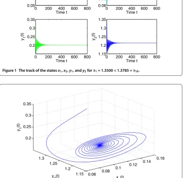
Figure 1 The track of the statesx1,x2,y1, andy2forτ1= 1.3500 < 1.3785 =τ10.
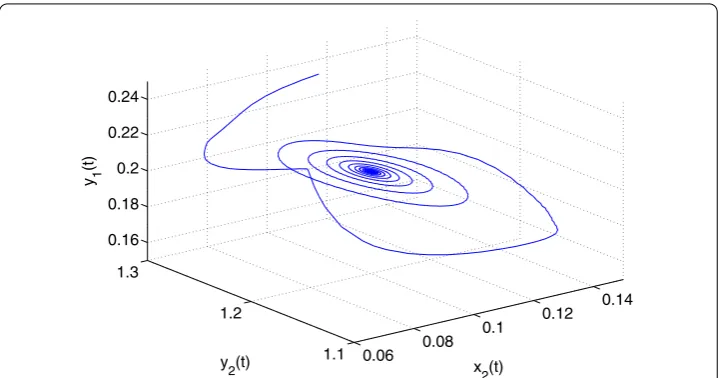
Figure 2 The phase plot of the statesx2,y1, andy2forτ1= 1.3500 < 1.3785 =τ10.
From (), we choose
¯
D= +qq¯∗+qq¯∗+qq¯∗+q
τ∗bq¯∗e–iω ∗ τ∗+τ∗
cq¯∗e–iω ∗ τ
+τ∗cqq¯∗e–i
ω∗τ∗– ,
such thatq∗,q= ,q∗,q¯= .
In the remainder of this section, we obtain the coefficients that can determine direction of the Hopf bifurcation and stability of the bifurcating periodic solutions by using the algorithms given in [] and using the computation process which is similar to that in []:
g= τ∗D¯
¯
q∗
a
q()()+aq()()q()() +aq()()q()
–τ∗ τ∗
+q¯∗a
q()(–)+aq()(–)q()(–)
Figure 3 The track of the statesx1,x2,y1, andy2forτ1= 1.3865 > 1.3785 =τ10.
Figure 4 The phase plot of the statesx2,y1, andy2forτ1= 1.3865 > 1.3785 =τ10.
g=τ∗D¯
¯
q∗
aq()()q¯()() +a
q()()q¯()() +q¯()()q()()
+a
q()()q¯()
–τ∗ τ∗
+q¯()()q()
–τ∗ τ∗
+q¯∗aq()(–)q¯()(–)
+a
q()(–)q¯()(–) +q¯()(–)q()(–),
g= τ∗D¯
¯
q∗
a
¯
q()()+aq¯()()q¯()() +aq¯()()q¯()
–τ∗ τ∗
+q¯∗a
¯
q()(–)+aq¯()(–)q¯()(–)
,
g= τ∗D¯
¯
q∗(a
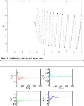
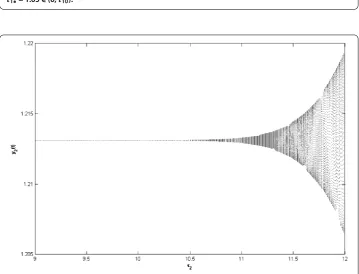
Figure 5 The bifurcation diagram with respect toτ1.
Figure 6 The track of the statesx1,x2,y1, andy2forτ2= 7.7750 < 8.7835 =τ20.
+a
W()()q()() + W
()
()q¯()() +W ()
()q()()
+ W
()
()q¯()()
+a
W()()q()
–τ∗ τ∗
+ W
() ()q¯()
–τ∗ τ∗
+W()
–τ∗ τ∗
q()() +W()
–τ∗ τ∗
¯
q()()
+a
q()()q¯()()
+ q()()q()()q¯()()+ a
q()()q¯()())
+q¯∗(a
Figure 7 The phase plot of the statesx2,y1, andy2forτ2= 7.7750 < 8.7835 =τ20.
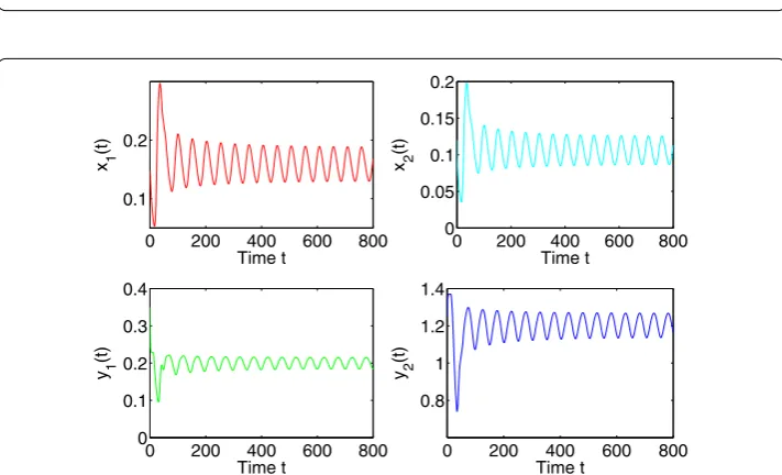
Figure 8 The track of the statesx1,x2,y1, andy2forτ2= 12.8050 > 8.7835 =τ20.
+a
W()(–)q()(–) + W
()
(–)q¯()(–) +W ()
(–)q()(–)
+ W
()
(–)q¯()(–)
+a
q()(–)q¯()(–)
+ q()(–)q()(–)q¯()(–)+ a
q()(–)q¯()(–))
,
with
W(θ) =
igq()
ω∗τ∗ e iω∗τ∗θ
+ig¯q¯() ω∗τ∗ e
–iω∗τ∗θ +Eeiω
∗ τ∗θ,
W(θ) = – igq()
ω∗τ∗ e
iω∗τ∗θ+ig¯q¯() ω∗τ∗ e
–iω∗τ∗θ+E
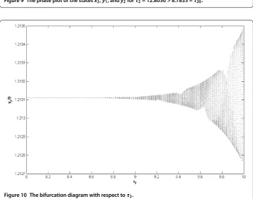
Figure 9 The phase plot of the statesx2,y1, andy2forτ2= 12.8050 > 8.7835 =τ20.
Figure 10 The bifurcation diagram with respect toτ2.
whereEandEcan be computed as the following equations, respectively: ⎛
⎜ ⎜ ⎜ ⎝
iω∗–a –a
–a iω∗–a–be–iω ∗
τ∗ –a
–ce–iω ∗
τ∗ iω∗
–a –ce–iω ∗ τ∗
–a iω∗–a
⎞ ⎟ ⎟ ⎟ ⎠E=
⎛ ⎜ ⎜ ⎜ ⎝
E() E()
⎞ ⎟ ⎟ ⎟ ⎠,
⎛ ⎜ ⎜ ⎜ ⎝
a a
a a+b a
c a c
a a
⎞ ⎟ ⎟ ⎟ ⎠E= –
⎛ ⎜ ⎜ ⎜ ⎝
E() E()
Figure 11 The track of the statesx1,x2,y1, andy2forτ= 1.3820 < 1.4126 =τ0.
Figure 12 The phase plot of the statesx2,y1, andy2forτ= 1.3820 < 1.4126 =τ0.
with
E() =a
q()()+aq()()q()() +aq()()q()
–τ∗ τ∗
,
E() =a
q()(–)+aq()(–)q()(–),
E() = aq()() +a
q()()q¯()() +q¯()()q()()
+a
q()()q¯()
–τ∗ τ∗
+q¯()()q()
–τ∗ τ∗
,
E() = aq()(–)q¯()(–) +a
Figure 13 The track of the statesx1,x2,y1, andy2forτ= 1.4375 > 1.4126 =τ0.
Figure 14 The phase plot of the statesx2,y1, andy2forτ= 1.4375 > 1.4126 =τ0.
Therefore, we can calculate the following values:
C() = i
ω∗τ∗
gg– |g|–| g|
+g
, μ= –
Re{C()} Re{λ(τ∗)}, β= Re
C()
, T= –
Im{C()}+μIm{λ(τ∗)}
ω∗τ∗ .
()
Based on the discussion above, we can obtain the following results.
Theorem For system(),ifμ> (μ< ),then the Hopf bifurcation is supercritical
Figure 15 The bifurcation diagram with respect toτ.
Figure 16 The track of the statesx1,x2,y1,y2forτ2= 8.7325 <τ2∗= 10.3472 andτ1∗= 1.05∈(0,τ10).
4 Numerical example
In this section, we give a numerical example to support the theoretical results in Section and Section . We consider the following system:
⎧ ⎪ ⎪ ⎪ ⎨ ⎪ ⎪ ⎪ ⎩
dx(t)
dt = x(t) – x(t) –x(t), dx(t)
dt = x(t) – .x(t) – xx(t–τ) –
.x(t)y(t) +.x(t) ,
dy(t)
dt =
.x(t–τ)y(t–τ)
+.x(t–τ) – .y(t) – .y(t),
dy(t)
dt = .y(t) – .y(t),
Figure 17 The phase plot of the statesx2,y1, andy2x1,x2,y1,y2forτ2= 8.7325 <τ2∗= 10.3472 and τ1∗= 1.05∈(0,τ10).
Figure 18 The track of the statesx1,x2,y1,y2forτ2= 12.3642 >τ2∗= 10.3472 andτ1∗= 1.05∈(0,τ10).
which has a unique positive equilibrium E∗(., ., ., .).
We haveτ> ,τ= . By some complex computations, we obtainω= .,τ=
.. Further, we havef(v∗) = . > . Thus, the conditions (H) and (H) hold.
According to Theorem , the positive equilibriumE∗of system () is asymptotically sta-ble whenτ<τ. This property can be illustrated by Figures and . However, onceτ
passes through the critical valueτ, the positive equilibriumE∗of system () will lose its
stability and a Hopf bifurcation occurs and a family of periodic solutions bifurcate from the positive equilibriumE∗of system (), which can be shown as in Figures and . This property can also be seen from the bifurcation diagram with respect toτin Figure .
Sim-ilarly, we haveω= .,τ= . forτ= ,τ> . The corresponding waveforms,
Figure 19 The phase plot of the statesx2,y1, andy2x1,x2,y1,y2forτ2= 12.3642 >τ2∗= 10.3472 and τ1∗= 1.05∈(0,τ10).
Figure 20 The bifurcation diagram with respect toτ2andτ1= 1.05.
We have τ =τ=τ > . We can obtain ω= . and then we get τ = ..
From Theorem , we can conclude that when τ increases from zero toτ the positive
equilibriumE∗ of system () is asymptotically stable, then it will lose its stability and a Hopf bifurcation occurs once τ >τ. As can be seen from Figures and , when
τ = .∈(, .), the positive equilibriumE∗of system () is asymptotically sta-ble. However, if we letτ= . >τ= ., the positive equilibriumE∗of system ()
We haveτ> and τ= .∈(,τ). We can obtainω∗= .,τ∗ = .. By
Theorem , the positive equilibriumE∗of system () is asymptotically stable whenτ∈
[,τ∗) and the positive equilibriumE∗ of system () becomes unstable whenτ>τ∗
and a family of periodic solutions bifurcate from the positive equilibriumE∗, which can be illustrated by Figures -.
Finally, by complex computations, we obtain C() = –. – .i, λ(τ∗) =
. – .i. Further, we can obtain μ = . > , β = –. < , T =
. > . According to Theorem , we know that the Hopf bifurcation of system () with respect toτwithτ= .∈(,τ) is supercritical, the bifurcating periodic solutions
are stable and increase.
5 Conclusion
In this paper, by incorporating the feedback delay of the mature prey and the time delay due to the gestation of the mature predator into the system considered in the literature [], we get a delayed predator-prey system with stage structure for both the predator and the prey, which is an extension of the literature []. Compared with the literature [], we mainly consider the effects of the two delays on the predator-prey system.
By regarding the possible combination of the two delays as the bifurcation parameter, and analyzing the characteristic equation of the linearized system at the positive equilib-rium, the sufficient conditions for the local stability of the positive equilibrium and the existence of a Hopf bifurcation are established. It has been shown that when the value of the delay is below the corresponding critical value, the system is asymptotically sta-ble. However, once the value of the delay is greater than the corresponding critical value, there will be a Hopf bifurcation at the positive equilibrium of the system and a family of periodic solutions occur. For the further investigation, formulas are derived to determine direction of the Hopf bifurcation and the stability of the bifurcating periodic solutions by using the normal form theory and center manifold theorem. From the numerical simula-tions, one can conclude that the species in system () could coexist in an oscillatory mode with some available delays of the mature prey and the mature predator under some certain conditions. This is valuable from the point of view of ecology.
Competing interests
The author declares that they have no competing interests.
Author’s contributions
The author read and approved the final manuscript.
Acknowledgements
The author would like to thank the editor and the anonymous referees for their work on the paper. This work was supported by Anhui Provincial Natural Science Foundation under Grant (No. 1508085QA13).
Received: 27 December 2014 Accepted: 9 June 2015 References
1. Xu, R, Chaplain, MAJ, Davidson, FA: Persistence and global stability of a ratio-dependent predator-prey mode with stage structure. Appl. Math. Comput.158, 729-744 (2004)
2. Liu, SQ, Beretta, E: A stage-structured predator-prey model of Beddington-DeAngelis type. SIAM J. Appl. Math.66, 1101-1129 (2006)
3. Kar, TK, Pahari, UK: Modelling and analysis of a prey-predator system with stage-structure and harvesting. Nonlinear Anal., Real World Appl.8, 601-609 (2007)
4. Liu, SQ, Zhang, JH: Coexistence and stability of predator-prey model with Beddington-DeAngelis functional response and stage structure. J. Math. Anal. Appl.342, 446-460 (2008)
6. Chakraborty, K, Jana, S, Kar, TK: Global dynamics and bifurcation in a stage structured prey-predator fishery model with harvesting. Appl. Math. Comput.218, 9271-9290 (2012)
7. Li, F, Li, HW: Hopf bifurcation of a predator-prey model with time delay and stage structure for the prey. Math. Comput. Model.55, 672-679 (2012)
8. Liu, M, Wang, K: Global stability of stage-structured predator-prey models with Beddington-DeAngelis functional response. Commun. Nonlinear Sci. Numer. Simul.16, 3792-3797 (2011)
9. Wang, LS, Feng, GH: Global dynamics of a predator-prey model with stage structure and Holling type-II functional response. Math. Appl.26, 765-773 (2013)
10. Ferrara, M, Guerrini, L, Bisci, GM: Center manifold reduction and perturbation method in a delayed model with a mound-shaped Cobb-Douglas production function. Abstr. Appl. Anal.2013, Article ID 738460 (2013) 11. Dong, T, Liao, XF, Li, HQ: Stability and Hopf bifurcation in a computer virus model with multistate antivirus. Abstr.
Appl. Anal.2012, Article ID 841987 (2012)
12. Bianca, C, Ferrara, M, Guerrini, L: Hopf bifurcations of a delayed-energy-based model of capital accumulation. Appl. Math. Inf. Sci.7, 139-143 (2013)
13. Zhang, JF: Bifurcation analysis of a modified Holling-Tanner predator-prey model with time delay. Appl. Math. Model.
36, 1219-1231 (2012)
14. Bianca, C, Ferrara, M, Guerrini, L: The Cai model with time delay: existence of periodic solutions and asymptotic analysis. Appl. Math. Inf. Sci.7, 21-27 (2013)
15. Meng, XY, Huo, HF, Xiang, H: Hopf bifurcation in a three-species system with delays. J. Appl. Math. Comput.35, 635-661 (2011)
16. Cui, GH, Yan, XP: Stability and bifurcation analysis on a three-species food chain system with two delays. Commun. Nonlinear Sci. Numer. Simul.16, 3704-3720 (2011)
17. Meng, XY, Huo, HF, Zhang, XB, Xiang, H: Stability and Hopf bifurcation in a three-species system with feedback delays. Nonlinear Dyn.64, 349-364 (2011)
18. Xu, CJ, Tang, XH, Liao, MX: Stability and bifurcation analysis on a ring of five neurons with discrete delays. J. Dyn. Control Syst.19, 237-275 (2013)
19. Xu, CJ, Tang, XH, Liao, MX: Stability and bifurcation analysis of a six-neuron BAM neural network model with discrete delays. Neurocomputing74, 689-707 (2011)
20. Zhao, M: Hopf bifurcation analysis for a semiratio-dependent predator-prey system with two delays. Abstr. Appl. Anal.
2013, Article ID 495072 (2013)
21. Zhang, ZZ, Yang, HZ, Fu, M: Hopf bifurcation in a predator-prey system with Holling type III functional response and time delays. J. Appl. Math. Comput.44, 337-356 (2014)
22. Li, XL, Wei, JJ: On the zeros of a fourth degree exponential polynomial with applications to a neural network model with delays. Chaos Solitons Fractals26, 519-526 (2005)