Implicit methods for the first derivative of the solution to heat equation

(1)

R E S E A R C H

Open Access

Implicit methods for the ﬁrst derivative of

the solution to heat equation

Suzan C. Buranay

1*

_{and Lawrence A. Farinola}

1

*_{Correspondence:}

[email protected]

1_{Department of Mathematics,}

Faculty of Arts and Sciences, Eastern Mediterranean University, Famagusta, North Cyprus, Turkey

Abstract

We propose special difference problems of the four point scheme and the six point symmetric implicit scheme (Crank and Nicolson) for the first partial derivative of the solutionu(x,t) of the first type boundary value problem for a one dimensional heat equation with respect to the spatial variablex. A four point implicit difference problem is proposed under the assumption that the initial function belongs to the Hölder spaceC5+α_{, 0 <}

_α

_{< 1, the nonhomogeneous term given in the heat equation}

is from the Hölder spaceC3+α, 3+α

2

x,t , the boundary functions are fromC 5+α

2 , and

between the initial and boundary conditions the conjugation conditions up to second order (q= 0, 1, 2) are satisﬁed. When the initial function belongs toC7+α_{, the}

nonhomogeneous term is fromC5+α, 5+α

2

x,t , the boundary functions are fromC 7+α

2 and

the conjugation conditions up to third order (q= 0, 1, 2, 3) are satisfied, a six point implicit difference problem is given. It is proven that the solution of the given four point and six point difference problems converge to the exact value of∂_∂u_xon the grids of orderO(h2₊

_τ

_{) and}_O₍_h2₊

_τ

2_{), respectively, where}_h_{is the step size in spatial} variablexand

τ

is the step size in time. Theoretical results are justiﬁed by numerical examples.

MSC: 65M06; 65M12; 65M22

Keywords: Finite diﬀerence method; Approximation of derivatives; Uniform error; Heat equation

1 Introduction

In science, especially in mathematical physics, not only the calculation of the solution of the differential equation but also the calculation of the first and second derivatives of the solution is very important to provide information about some physical phenomena [1]. For example, Tuttle [2] in a theory of the drying wood adopts the fundamental hypothesis that the rate of which transfusion takes place transversely with respect to the wood fibers (∂θ

∂t)

is proportional to the slope of the moisture gradient (∂_∂2_xθ2), whereθis the moisture content

expressed as a percentage of the oven-dry weight of the wood. Therefore, accurate approx-imation of∂θ

∂xis very important to provide information about the moisture gradient. Since

the differentiation operation is ill-conditioned, to find a highly accurate approximation for the derivatives of the solution of a differential equation is problematic.

In [3] the uniform convergence of the diﬀerence derivatives over the whole grid do-main to the corresponding derivatives of the exact solution for the two dimensional

(2)

Laplace equation with orderO(h2_{) is proved. In [4], under the conditions that the} bound-ary functions belong to C6,λ_{, 0 <}_λ_{< 1, on the sides of the rectangle and are} con-tinuous on the vertices and second, fourth order derivatives satisfy the compatibility conditions on the vertices which result from the Laplace equation, difference schemes are constructed for the first and pure second order derivatives of the solution. It is proved that the order of convergence of the solutions of these difference schemes is O(h4_).

For the 3D Laplace equation on a rectangular parallelepiped, recent studies are given in [5] and [6] and the constructed diﬀerence schemes converge with the order ofO(h2_{) and}

O(h4_{), respectively, to the first and pure second derivatives of the exact solution of the 3D} Dirichlet problem. It is assumed in [5] that the fourth derivatives of the boundary func-tions on the faces of a parallelepiped satisfy the Hölder condition, and on the edges their second derivatives satisfy the compatibility condition, whereas in [6] they are assumed to have sixth order derivatives satisfying the Hölder condition on the faces, and their second and fourth order derivatives satisfy the compatibility conditions on the edges. Most re-cently, in [7] difference schemes on a cubic grid for obtaining the solution of the Dirichlet problem for the 3D Laplace equation on a rectangular parallelepiped, its first and pure sec-ond derivatives difference schemes are constructed and the approximate values of the first and pure second derivatives converge with ordersO(h6|lnh|) andO(h5+λ_{), 0 <}_λ_{< 1,} re-spectively. It is assumed that the boundary functions on the faces have seventh derivatives satisfying the Hölder condition and on the edges their second, fourth and sixth derivatives satisfy the compatibility condition. At the same time in [8], anO(hp–1_),_p_∈_{[4, 5] order of} approximation for the first order derivatives of the solution of the 3D Laplace equation is proven under a weaker assumption on the smoothness of the boundary functions on the faces of the parallelepiped than those used in [6].

In this study special difference problems of four point and six point symmetric im-plicit difference schemes for the derivative of the solutionu(x,t) of the first type boundary value problem for one dimensional heat equation with respect to the spatial variablexare proposed. For the construction of the four point implicit difference problem we require that:

(a) the initial function belongs toC5+α_{, the nonhomogeneous term given in the heat}

equation is fromC3+α,

3+α

2

x,t , the boundary functions are fromC

5+α

2 _{, and the}

conjugation conditions of ordersq= 0, 1, 2are satisﬁed at the corners of the boundary. For the construction of the six point implicit diﬀerence problem it is assumed that:

(b) the initial function belongs toC7+α_{, the nonhomogeneous term is from}_C5+α,5+2α

x,t , the

boundary functions are fromC7+2α, and the conjugation conditions of orders

q= 0, 1, 2, 3are satisﬁed.

(3)

constructed difference scheme converges uniformly to the exact value of ∂_∂u_x on the grids of orderO(h2₊_τ_{) where}_h_{is the step size in spatial variable}_x_and_τ _{is the step size in} time. In Sect.4, we require that the boundary value problem satisfies the conditions (b) hence, a special six point implicit difference problem for the approximation of ∂u

∂x is

pro-posed. Uniform convergence of orderO(h2+τ2) for this scheme is shown. In Sect.5, to justify the theoretical results numerical examples are constructed and obtained results are presented via tables and ﬁgures. In Sect.6, concluding remarks are given.

2 Implicit difference solution of ﬁrst type boundary value problem for one dimensional heat equation

2.1 Basic notations and ﬁrst type boundary value problem

Based on Section 5, Chapter IV in [10], we give the following deﬁnitions. We denote by

L(x,t, ∂ ∂x,

∂

∂t) the linear parabolic diﬀerential operator with real coeﬃcients

L

LetΩbe a bounded domain inn-dimensional Euclidean spaceEn. It is assumed that the

coeﬃcients of the operator of (1) are deﬁned in a layerD=En×(0,T). In the

cylindri-Letqbe a non-negative integer. We use the notations

(4)

The conjugation (compatibility) conditions up to orderm≥0 are

ous inQtogether with all derivatives of the form∂j0

t ∂ j

xfor 2j0+j<sand have ﬁnite norm deﬁned inCs_x,_,s_t/2(Q).Cs₍_Ω_{) is the Hölder space whose elements are continuous functions}

g(x) inΩ having inΩ continuous derivatives up to order [s] inclusively, and have ﬁnite norm deﬁned inCs₍_Ω_{) (see [10]).}

Theorem 1(From Theorem 5.2, Section 5, Chapter IV in [10]) Suppose s> 0is a

non-integer number, the coeﬃcients of the operatorL belongs to the class Cs, s

2.2 Implicit difference solution of one dimensional problem

TakeΩ= (0,b),σT= (0,T), andΩ,σTare the closure of these sets respectively, alsoQT=

dxk to present thekth partial and ordinary derivatives respectively with respect to time variablet, spatial variablex. We consider the ﬁrst type boundary value problem for a one dimensional heat equation:

(5)

Furthermore, the conjugation conditions up to orderm≥0 in (10) for the one dimensional

(i) The boundary value problem (11)–(13) satisfying the conditions

u0(x)∈C5+α(Ω), f(x,t)∈C (ii) The boundary value problem (11)–(13) satisfying the conditions

u0(x)∈C7+α(Ω), f(x,t)∈C

Proof The proof of Theorem2follows from Theorem1.

(6)

respectively. Assume thatc1,c2, . . . are positive constants independent fromhandτ; in each section, those constants are enumerated anew. For the numerical solution of the Problem1(i), we use the four point difference problem (= 3) and for the numerical solu-tion of the Problem1(ii), we use the six point symmetric difference problem (= 6) [9]. We denote the solution of these difference problems byuand use the notationsu0_m=u(xm, 0)

onωh,0,u0j =u(0,tj) onω0,τ, anduj_N=u(b,tj) onωb,τ. The diﬀerence schemes are as follows: uh_t_,,_mτ =aΘuh,τ

m +Φfh,τ onωh,τ, = 3 or = 6, (28)

u0_m=u0(xm) onωh,0, (29)

uj₀=u1(tj) onω0,τ, uj_N =u2(tj) onωb,τ, (30)

where

uh_t_,,_mτ =1

τ

uj_m+1–uj_m, (31)

Θ3uh_m,τ= 1 h2

uj_m+1_–1– 2u_mj+1+uj_m+1₊₁, (32)

Θ6uh_m,τ= 1 2h2

uj_m+1_–1– 2u_mj+1+uj_m+1₊₁+ 1 2h2

uj_m_–1– 2u_mj +uj_m₊₁, (33)

Φfh,τ= ⎧ ⎨ ⎩

f(xm,tj+1) if= 3,

f=f(xm,tj+1₂) if= 6.

(34)

The operatorΘ3uh,τ

m is the central diﬀerence formula andΘ6uhm,τ is the averaging central

diﬀerence formula with three points and six points respectively, for approximating∂_x2u. Heret_j₊1

2 =tj+ 0.5τ,f(x,t) is the given function in (11) andu0(x) given in (12),u1(t),u2(t)

given in (13) are the initial and boundary functions, respectively. Consider the following systems:

qh_t_,,_mτ =aΘq_mh,τ+gh,τ onωh,τ, = 3 or = 6, (35)

q0_m= 0 onωh,0, (36)

qj₀= 0 onω0,τ, qj_N= 0 onωb,τ (37) qh_t_,,_mτ =aΘqh_m,τ+gh,τ onωh,τ, = 3 or = 6, (38)

q0_m≥0 onωh,0, (39)

qj₀≥0 onω0,τ, qj_N≥0 onωb,τ (40)

wheregh,τ_,_gh,τ

are given functions and|gh,τ_{| ≤}_gh,τ

onωh,τ alsoq_th_,,_mτ,qh_t_,,_mτ are diﬀerence formulae analogous to (31) andΘ_qh,τ

m ,Θqh,

τ

m are diﬀerence formulae analogous to (32)

or (33) for= 3 or= 6, respectively.

Lemma 3 The solutionq of the system(35)–(37)and the solution q of the system(38)–(40) satisfy the inequality

(7)

for any r by the four point implicit scheme(= 3)and for r≤1,by the six point symmetric

Chap. 4 in [9]) because the coefficients of the finite difference schemes (42) and (43) satisfy all conditions of the comparison theorem for anyrand forr≤1, respectively.

Lemma 4 For the solution of the problem

qh_t_,,_mτ =aΘq_mh,τ+β onωh,τ, = 3 or = 6, (44)

q0_m= 0 onωh,0, (45)

qj₀= 0 onω0,τ, qj_N = 0 onωb,τ, (46)

the following inequality holds true:

(8)

Proof For the four point implicit scheme (= 3), we consider the functions

For the six point symmetric implicit scheme (= 6), we consider the functions

q6₁(x,t) =1

satisﬁes the following pointwise estimation:

|u–u| ≤c1Υ

h2+τ, (54)

for any value of r where u is the exact solution of Problem1(i).The solutionu of the six point finite difference problem(28)–(30) (= 6)satisfies the following pointwise estimation:

|u–u| ≤c2Υ

h2+τ2, (55)

for r≤1where u is the exact solution of Problem1(ii).

Proof On the basis of Theorem 2, the exact solution u of Problem 1(i) belongs to

C5+α, From Theorem2, the exact solutionuof Problem1(ii) belongs toC7+α,

7+α

2

(9)

the derivatives∂4

xu,∂t3uare bounded up to the boundary. The error functionεuh,τ satisﬁes

the following diﬀerence problem:

εh_u,_,τ_t_,_m=aΘ6εh_u_,,τ_m+ψu onωh,τ, (59)

ε0_u_,_m= 0 onωh,0, (60)

εj_u_,0= 0 onω0,τ, ε

j

u,N= 0 onωb,τ. (61) Using Taylor’s formula for the functionu(x,t) about the node (xm,tj+1₂) shows thatψu=

O(h2+τ2). Applying Lemma3to the six point implicit diﬀerence problem (44)–(46) (= 6) and (59)–(61) and on the basis of Lemma4we obtain|εh,τ

u | ≤c2Υ(h2+τ2). 3 Implicit four point difference approximation of

∂

xu

Problem 2

(i) Given the Problem1(i), we denotepi=∂xuonγi,i= 1, 2, 3and set up the next

boundary value problem forv=∂xu,

Lv=∂xf(x,t) onQT, (62)

v(x, 0) =p2 onγ2, (63)

v(0,t) =p1 onγ1, v(b,t) =p3 onγ3, (64)

wheref(x,t)is the given function in (11). We take

p1h=

1 2h

–3u1(t) + 4u(h,t) –u(2h,t)

onω0,τ, (65)

p2h=∂xu0(x) onωh,0, (66)

p3h=

1 2h

3u2(t) – 4u(b–h,t) +u(b– 2h,t)

onωb,τ, (67)

andu0(x)given in (12),u1(t),u2(t)given in (13) are the initial and boundary functions, respectively,uis the solution of the four point diﬀerence problem (28)–(30) (= 3).

Lemma 6 The following inequality holds:

pih(u) –pih(u)≤c1

h2+τ, i= 1, 3, (68)

where u is the solution of the diﬀerential Problem1(i)andu is the solution of the four point diﬀerence problem(28)–(30) (= 3).

Proof Taking into consideration Theorem2, and using (65) and (67) and Theorem5, we have

_p_ih₍_u_{) –}_p_ih₍_u₎_≤ 1 2h

4(c2h)

h2+τ+ (c22h)

h2+τ≤c1

h2+τ, i= 1, 3. (69)

(10)

Lemma 7 The following inequality is true:

max

ω0,τ∪ωb,τ

pih(u) –pi≤c3

h2+τ, i= 1, 3, (70)

whereu is the solution of the four point diﬀerence problem(28)–(30) (= 3).

Proof On the basis of Theorem2, the exact solutionu∈C5+α,

5+α

2

x,t (QT). Then at the end

points (0,σ τ)∈ω0,τ and (b,σ τ)∈ωb,τ of each line segment [(x,t) : 0≤x≤b, 0 <t≤T] (65) and (67) give the second order approximation of∂xu, respectively. From the

trunca-tion error formula (see [11]) it follows that

max

ω0,τ∪ωb,τ

pih(u) –pi≤

h2 3 maxQT

∂_x3u≤c3h2, i= 1, 3. (71)

Using Lemma6and the estimation (66), (71) follows.

We construct the following diﬀerence problem for the numerical solution of Prob-lem2(i):

vh_t_,,_mτ =aΘ3v_mh,τ+Φ∂xfh,τ onωh,τ, (72)

v0_m=p2h onωh,0, (73)

vj₀=p1h(u) onω0,τ, vj_N=p3h(u) onωb,τ, (74)

where thepihare deﬁned by (65)–(67) andΦ∂xfh,τ =∂xf|(xm,tj+1) anduis the solution of

the four point diﬀerence problem (28)–(30) (= 3).

Theorem 8 The solutionv of the finite difference problem(72)–(74)satisfies

max

ωh,τ

|v–v| ≤c4

h2+τ, (75)

where v=∂xu is the exact solution of Problem2(i).

Proof Let

εh_v,τ =v–v onωh,τ, (76)

wherev=∂xu. Denote byεvh,τ=maxω_h_,_τ|v–v|. From (72)–(74) and (76) we have

εh,τ

v,t,m=aΘ

3_εh,τ

v,m+ψv onωh,τ, (77)

ε0_v_,_m= 0 onωh,0, (78)

εj_v_,0=p1h(u) –v onω0,τ, ε

j

v,N=p3h(u) –v onωb,τ, (79) whereψv=aΘ3v–vt,m+Φ∂xfh,τ. We take

(11)

where

ε1,_v_,_th_,,_mτ=aΘ3ε1,_v_,_mh,τ onωh,τ, (81)

ε1,0_v_,_m= 0 onωh,0, (82)

ε1,_v_,0j=p1h(u) –v onω0,τ, ε 1,j

v,N=p3h(u) –v onωb,τ, (83)

ε2,_v_,_th_,_m,τ=aΘ3ε_v2,_,_mh,τ+ψv onωh,τ, (84)

ε2,0_v_,_m= 0 onωh,0, (85)

ε_v2,_,0j= 0 onω0,τ, ε_v2,_,_Nj = 0 onωb,τ. (86)

From Lemma7and by maximum principle for the solution of the system (81)–(83) we have

max

ωh,τ

ε1,_vh,τ≤max

i=1,3 maxωh,τ

pih(u) –v≤c4

h2+τ. (87)

The solutionε2,h,τ

v of system (84)–(86) is the error of the approximate solution obtained

by the ﬁnite diﬀerence method for the boundary value Problem2(i) when the boundary values satisfy the conditions

p2∈C4+α(Ω), ∂xf(x,t)∈C

2+α,1+α2

x,t (QT), pi∈C2+

α

2₍_σ_T_), _i_{= 1, 3,} ₍₈₈₎

⎧ ⎨ ⎩

p(₁q)(0) =v(q)_(0),

p(₃q)(0) =v(q)₍_b_), q= 0, 1, 2. (89)

Since the functionv=∂xusatisﬁes Eq. (62) with the initial functionp2onγ2and bound-ary functionsp1,p3 onγ1 andγ3, respectively, and on the basis of Theorem1and the maximum principle, we obtain

max

ωh,τ

ε2,_vh,τ≤c5

h2+τ, (90)

and using (80), (87) and (90) we obtain (75).

4 Implicit six point symmetric difference approximation of

∂

xu

Problem 2

(ii) Given the Problem1(ii), we denotepi=∂xuonγi,i= 1, 2, 3and set up the boundary

value problem (62)–(64) forv=∂xu.

Lemma 9 The following inequality holds:

pih(u) –pih(u)≤c1

h2+τ2, i= 1, 3, (91)

(12)

Proof On the basis of Theorem2, and from (65), (67) and using Theorem5, we have

pih(u) –pih(u)≤

1 2h

4(c2h)

h2+τ2+ (c22h)

h2+τ2

≤c1

h2+τ2, i= 1, 3. (92)

Lemma 10 The following inequality is true:

max

ω0,τ∪ωb,τ

pih(u) –pi≤c3

h2+τ2, i= 1, 3, (93)

whereu is the solution of the six point diﬀerence problem(28)–(30) (= 6)for r≤1.

Proof Using Theorem2, the proof is analogous to the proof of Lemma7.

We propose the following six point diﬀerence problem for the numerical solution of Problem2(ii):

vh_t_,,_mτ =aΘ6v_mh,τ+Φ∂xfh,τ onωh,τ, (94)

v0_m=p2h onωh,0, (95)

vj₀=p1h(u) onω0,τ, v

j

N=p3h(u) onωb,τ, (96) wherepihare deﬁned by (65)–(67) andΦ∂xfh,τ=∂xf|(xm,t_j_{+ 1}

2

)anduis the solution of the six point diﬀerence problem (28)–(30) (= 6) forr≤1.

Theorem 11 For r≤1,the solutionv of the finite difference problem(94)–(96)satisfies

max

ω_h,τ

|v–v| ≤c4

h2+τ2, (97)

where v=∂xu is the exact solution of Problem2(ii).

Proof The proof is analogous to the proof of Theorem8. From (94)–(96) and (76) we have

εh_v_,,_tτ_,_m=aΘ6εh_v_,,_mτ +ψv onωh,τ, (98)

ε0_v_,_m= 0 onωh,0, (99)

εj_v_,0=p1h(u) –v onω0,τ, ε_vj_,_N=p3h(u) –v onωb,τ, (100)

whereψv=aΘ6v–vt,m+Φ∂xfh,τ. We take

ε_vh,τ =ε_v1,h,τ+ε2,_vh,τ, (101)

where

(13)

ε1,0_v_,_m= 0 onωh,0, (103) ε1,_v_,0j=p1h(u) –v onω0,τ, ε

1,j

v,N=p3h(u) –v onωb,τ, (104)

ε2,_v_,_th_,_m,τ=aΘ6ε_v2,_,_mh,τ+ψv onωh,τ, (105)

ε2,0_v_,_m= 0 onωh,0, (106)

ε_v2,_,0j= 0 onω0,τ, ε_v2,_,_Nj = 0 onωb,τ. (107) From Lemma10and by the maximum principle for the solution of the system (102)–(104) we have

max

ωh,τ

ε1,_vh,τ≤max

i=1,3maxωh,τ

pih(u) –v≤c4

h2+τ2. (108)

The solutionε_v2,h,τof system (105)–(107) is the error of the approximate solution obtained by the ﬁnite diﬀerence method for the boundary value Problem2(ii) when the boundary values satisfy the conditions

p2∈C6+α(Ω), ∂xf(x,t)∈C

4+α,2+α₂

x,t (QT), pi∈C3+

α

2₍_σ

T),i= 1, 3, (109)

⎧ ⎨ ⎩

p(₁q)(0) =v(q)_(0),

p(₃q)(0) =v(q)₍_b_), q= 0, 1, 2, 3, . . . . (110) Since the functionv=∂xusatisﬁes Eq. (62) with the initial functionp2onγ2and boundary functionsp1,p3onγ1andγ3, respectively and on the basis of Theorem1and the maximum principle in Chap. 4 of [9] we obtain

max

ωh,τ

ε2,_vh,τ≤c5

h2+τ2 (111)

using (80), (108) and (111) we obtain (97).

5 Numerical aspects

Two problems are considered such that the first type boundary value problem for the one dimensional heat equation in Example 1 and in Example 2 are chosen as exam-ples for Problem1(i) and Problem1(ii), respectively, and the exact first derivatives of their solutions with respect to xare known. The third example is also given as an ex-ample of Problem 1(ii), however, the exact first derivative of the solution of this prob-lem with respect toxis not given. All the computations are carried out in double pre-cision using the Fortran programming language. For the constructed examples we take QT ={(x,t) : 0 <x< 1, 0 <t≤1}, γ1={(0,t) : 0≤t≤1}, γ2={(x, 0) : 0≤x≤1}, and γ3={(1,t) : 0≤t≤1}, and the constantain the operatorL≡∂∂t–a

∂2

∂x2 is taken asa= 1.

Example1

Lu=f(x,t) onQT,

u(x, 0) =x265 ₊_sin

π

2x

(14)

u(0,t) =t135 _on_γ₁_,

2x). Using the proposed implicit four point diﬀerence scheme (28)–(30) (= 3) we obtain the approximate solu-tionuby the applying the Gauss–Thomas method [12] for solving an algebraic system of equations at each time level with space step sizeh= 2–μ_{and time step size}_τ_{= 2}–λ_where

μ,λare positive integers. Next the boundary value problem forv=∂u

∂x is constructed

us-ing the obtained approximate solutionuand the proposed Problem2(i). Furthermore, the approximate solutionvof the diﬀerence problem (72)–(74) is obtained at the same grid points. The exact solution is known:v(x,t) = 26

ofvwith respect tohandτ for Example1. Table2represents the maximum errors for h= 2–9,τ = 2–λ_,_λ_{= 6, 7, 8, 9, 10, 11 and the order of convergence}

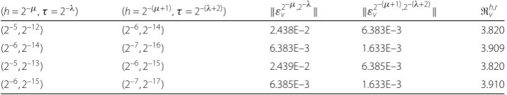
ofvwith respect toτfor Example1. According to the definition of the maximum error the third and fourth columns of Table1and Table2present the theoretical upper bound errors given in (75). Note that theO(h2₊_τ_{) order of convergence corresponds to} ₂2 _{of the} quantities defined by (113), and 21_{of the quantities defined by (114). Figure}₁_presents the error function|ε2–7,2–17

Table 1 Maximum errors and the order of convergence of approximate solutionv˜with respect toh

(15)

Table 2 Maximum errors and the order of convergence of approximate solutionv˜with respect toτ

for Example1

(h= 2–μ_,_τ_{= 2}–λ₎ ₍_h_{= 2}–μ_,_τ_{= 2}–(λ+1)₎ _ε2–μ,2–λ

v ε2–

μ_,2–(λ+1)

v τv

(2–9_{, 2}–6₎ ₍₂–9_{, 2}–7₎ _6.087E–2 _3.058E–2 _1.991

(2–9, 2–7) (2–9, 2–8) 3.058E–2 1.531E–2 1.997

(2–9_{, 2}–8₎ ₍₂–9_{, 2}–9₎ _1.531E–2 _7.634E–3 _2.006

(2–9, 2–9) (2–9, 2–10) 7.634E–3 3.791E–3 2.014

(2–9_{, 2}–10₎ ₍₂–9_{, 2}–11₎ _3.791E–3 _1.867E–3 _2.031

Figure 1The error function|ε2–7,2–17v |=|v–v|forh= 2–7, andτ= 2–17for Example1

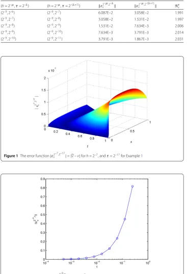
Figure 2The maximum errorsε2–9,v τforh= 2–9, with respect toτof Example1

u(0,t) = 5 18t

18

5 _on_γ₁_,

u(1,t) = 5 18t

18 5 ₊ 5

36 5 18cos

(16)

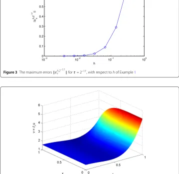
Figure 3The maximum errorsεh,2–17v forτ= 2–17, with respect tohof Example1

Figure 4The functionvpresenting the exact solution∂xufor Example1

wheref(x,t) = –₃₆5x365_t135 _sin₍_t185_{) +}_t135 _–31

18x

26

5 _cos₍_t185_{) +}π2

4 sin( πx

2). Using the proposed implicit six point diﬀerence scheme (28)–(30) (= 6) we obtain the approximate solution uby applying the Gauss–Thomas method [12] for solving algebraic system of equations at each time level for r= 2–ω_where_ω_{is nonnegative integer. Next the boundary value} problem for v= ∂_∂u_x is constructed from the proposed Problem2(ii) using the obtained approximate solutionu. Furthermore, the approximate solutionvfor∂_∂u_xis obtained at the same grid points by solving the system of equations using (94)–(96), and compared on the grids with the known exact solutionv(x,t) = 5

18x

31 5 cos(t

18 5) +π

2cos( πx

2 ). We use

h,τ

v =

ε2_v–μ,2–λ ε2v–(μ+1),2–(λ+1)

(116)

(17)

Figure 5The grid functionv2–7,2–17_{presenting the approximate solution}_v_of_∂x_u_when_h_{= 2}–7_,_τ_{= 2}–17_for Example1

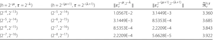
Table 3 Maximum errors and the order of convergence of approximate solutionv˜with respect toh

andτfor Example2

(h= 2–μ_,_τ_{= 2}–λ₎ ₍_h_{= 2}–(μ+1)_,_τ_{= 2}–(λ+1)₎ _ε2–μ,2–λ

v ε2–(

μ+1),2–(λ+1)

v h,vτ

(2–4_{, 2}–13₎ ₍₂–5_{, 2}–14₎ _1.0567E–2 _3.1449E–3 _3.360

(2–5_{, 2}–14₎ ₍₂–6_{, 2}–15₎ _3.1449E–3 _8.5353E–4 _3.685

(2–6_{, 2}–15₎ ₍₂–7_{, 2}–16₎ _8.5353E–4 _2.2209E–4 _3.843

(2–7_{, 2}–16₎ ₍₂–8_{, 2}–17₎ _2.2209E–4 _5.6628E–5 _3.922

maximum errors forh= 2–μ_,_μ_{= 4, 5, 6, 7, 8 and}_τ_{= 2}–λ_,_λ_{= 13, 14, 15, 16, 17, respectively,} and the ordersh,τ

v for Example2. The third and fourth columns of this table present the

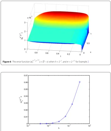
theoretical upper bound errors given in (97). Figure6presents the error function|ε_v2–7,2–17|

forh= 2–7_{, and}_τ _{= 2}–17_{for Example}_{2. The maximum errors}_εh,2–17

v whenτ= 2–17, with

respect toh, is demonstrated by Fig.7for Example2. Figure8shows the exact solution v(x,t) =∂xu, and the grid functionv2

–7_,2–17

presenting the approximate solutionvof∂xu

whenh= 2–7_,_τ_{= 2}–17_{for Example}_2.

Example3

Lu=f(x,t) onQT,

u(x, 0) =e–x onγ2,

u(0,t) = 1 + 0.001t257 _on_γ

1,

u(1,t) = 0.0001sint257_{+ 0.001}_t257 ₊_e–1 _on_γ

3, (117)

wheref(x,t) = 0.000125₇x507_t187 _cos₍_t257 _{) + 0.001}25

7t

18

7 _{– 0.0001}50

7 43

7x

36

7 _sin₍_t257_{) –}_e–x_{. The}

(18)

us-Figure 6The error function|ε2–7,2–17v |=|v–v|whenh= 2–7, andτ= 2–17for Example2

Figure 7The maximum errorsεh,2–17v forτ= 2–17, with respect tohfor Example2

ing the obtained approximate solutionu; then the approximate solutionvofv=∂xuis

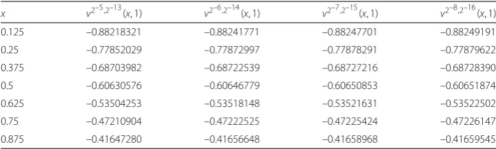
ob-tained at the same grid points by solving the system of equations resulting from (94)–(96). Letv2–μ,2–λ₍_x_,_t_{) be the approximate solution}_v_{at (}_x_,_t_{) when}_h_{= 2}–μ_and_τ_{= 2}–λ_{. The exact} solutionvis not given. To verify the order of convergence of the computed solutionvto the exact solutionvwe compute the solution at grid points with successively reduced step sizeshandτby a factor of two and the ratio of the absolute successive errors (see Chap. 2 of [13]). Table4presentsv2–μ,2–λ₍_x_,_t_{) at the grid points (0.125, 1), (0.25, 1), (0.375, 1), (0.5, 1),} (0.625, 1), (0.75, 1) and (0.875, 1) for the pairs (μ,λ) = (5, 13), (6, 14), (7, 15), (8, 16, ) which means that the step sizeshinxandτ intare halved successively. Table5demonstrates the absolute error ratios

r1=

v2–5,2–13(x, 1) –v2–6,2–14(x, 1) v2–6_,2–14

(x, 1) –v2–7_,2–15

(19)

Figure 8The exact solution∂xuand the grid functionv2–7,2–17_for_h_{= 2}–7_,_τ_{= 2}–17_{of Example}₂

Table 4 The approximate solutionv˜at some grid points ont= 1 for Example3

x v2–5,2–13₍_x_{, 1)} _v2–6,2–14₍_x_{, 1)} _v2–7,2–15₍_x_{, 1)} _v2–8,2–16₍_x_{, 1)}

0.125 –0.88218321 –0.88241771 –0.88247701 –0.88249191

0.25 –0.77852029 –0.77872997 –0.77878291 –0.77879622

0.375 –0.68703982 –0.68722539 –0.68727216 –0.68728390

0.5 –0.60630576 –0.60646779 –0.60650853 –0.60651874

0.625 –0.53504253 –0.53518148 –0.53521631 –0.53522502

0.75 –0.47210904 –0.47222525 –0.47225424 –0.47226147

0.875 –0.41647280 –0.41656648 –0.41658968 –0.41659545

r2=

v_v22–6–7,2_,2–15–14(x, 1) –v2–7,2–15(x, 1)

(x, 1) –v2–8_,2–16

(x, 1) ,

and the corresponding orders

p1=log2

v_v22–5–6,2_,2–14–13(x, 1) –v2–6,2–14(x, 1)

(x, 1) –v2–7_,2–15

(x, 1) ,

p2=log2

v_v22–6–7,2_,2–15–14(x, 1) –v2–7,2–15(x, 1)

(x, 1) –v2–8_,2–16

(x, 1) ,

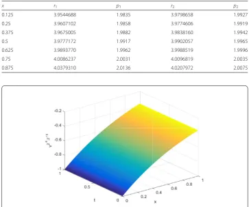
for the considered points att= 1. By analyzing the values ofp1andp2in the third and ﬁfth columns of Table5, respectively, we conclude that the order of convergence is quadratic in the two variablesxandtont= 1. Figure9illustrates the grid functionv2–8,2–16_presenting the approximate solutionvofv=∂xuwhenh= 2–8,τ= 2–16for Example3.

6 Concluding remarks

(20)

Table 5 The absolute error ratios at some grid points ont= 1 and the ordersp1,p2for Example3

x r1 p1 r2 p2

0.125 3.9544688 1.9835 3.9798658 1.9927

0.25 3.9607102 1.9858 3.9774606 1.9919

0.375 3.9675005 1.9882 3.9838160 1.9942

0.5 3.9777172 1.9917 3.9902057 1.9965

0.625 3.9893770 1.9962 3.9988519 1.9996

0.75 4.0086237 2.0031 4.0096819 2.0035

0.875 4.0379310 2.0136 4.0207972 2.0075

Figure 9The grid functionv2–8,2–16_{presenting the approximate solution}_v_of_∂x_u_when_h_{= 2}–8_,_τ_{= 2}–16_for Example3

a number of derivatives in the variablesxandtnecessary in this connection for perform-ing current and subsequent manipulation in approximatperform-ing∂u

∂x. We prove that the solution

of the proposed four point and six point diﬀerence schemes converge to the exact value of ∂u

∂xon the grids of orderO(h

2₊_τ_{) and}_O₍_h2₊_τ2_{), respectively.}

Remark12 These results can be used in some domain decomposition methods allowing for parallel computation [14,15]. Furthermore, the proposed approach may be applicable to similar equations, given in the phenomena of impact of a moving foot on the transfer of heat from a constantly heated warm water into the foot immersed within a footbath [16] and the enhancement of performance by increasing the thermal eﬃciency of a direct absorption solar collector based on an alimino-water nanoﬂuid [17].

Remark13 The proposed approach can also be applied to ﬁnding second order deriva-tives of the solution of the ﬁrst type boundary value problem for a one dimensional heat equation and this research will be presented in a subsequent article. Also the methodology may be extended to a two dimensional heat equation.

Acknowledgements

The authors thank Professor A.A. Dosiyev for his attention to this work and valuable advices.

Funding

(21)

Competing interests

The authors declare that they have no competing interests.

Authors’ contributions

The authors contributed equally to the writing of this paper. All authors read and approved the ﬁnal manuscript.

Publisher’s Note

Springer Nature remains neutral with regard to jurisdictional claims in published maps and institutional aﬃliations.

Received: 13 February 2018 Accepted: 12 November 2018

References

1. Bateman, H.: Partial Diﬀerential Equations of Mathematical Physics. Dover, New York (1944) 2. Tuttle, F.: A mathematical theory of the drying of wood. J. Franklin Inst.200, 609–614 (1925)

3. Volkov, E.A.: On convergence inC2of a diﬀerence solution of the Laplace equation on a rectangle. Russ. J. Numer. Anal. Math. Model.14(3), 291–298 (1999)

4. Dosiyev, A.A., Sadeghi, M.M.H.: A fourth order accurate approximation of the ﬁrst and pure second derivatives of the Laplace equation on a rectangle. Adv. Diﬀer. Equ.2015, Article ID 67 (2015).

https://doi.org/10.1186/s13662-015-0408-8

5. Volkov, E.A.: On the grid method by approximating the derivatives of the solution of the Dirichlet problem for the Laplace equation on the rectangular parallelpiped. Russ. J. Numer. Anal. Math. Model.19(3), 209–278 (2004) 6. Dosiyev, A.A., Sadeghi, M.M.H.: On a highly accurate approximation of the ﬁrst and pure second derivatives of the

Laplace equation in a rectangular parellelpiped. Adv. Diﬀer. Equ.2016, Article ID 145 (2016).

https://doi.org/10.1186/s13662-016-0868-5

7. Dosiyev, A.A., Abdussalam, A.: On the high order convergence of the diﬀerence solution of Laplace’s equation in a rectangular parallelepiped. Filomat32(3), 893–901 (2018)

8. Dosiyev, A.A., Sarikaya, H.: 14-point diﬀerence operator for the approximation of the ﬁrst derivatives of a solution of Laplace’s equation in a rectangular parallelepiped. Filomat32(3), 791–800 (2018)

9. Samarskii, A.A.: The Theory of Diﬀerence Schemes. Dekker, New York (2001)

10. Ladyženskaja, O.A., Solonnikov, V.A., Ural’ceva, N.N.: Linear and Quasi-Linear Equations of Parabolic Type. Translation of Mathematical Monographs, vol. 23. Am. Math. Soc, Providence (1967)

11. Burden, R.L., Faires, J.D.: Numerical Analysis. Cengage Learning, Boston (2011)

12. Fausett, L.V.: Applied Numerical Analysis Using Matlab. Pearson Prentice Hall, Upper Saddle River (2008) 13. Einarsson, B.: Accuracy and Reliability in Scientiﬁc Computing. SIAM, Philadelphia (2005)

14. Kuznetsov, Y.: New algorithms for approximate realization of implicit diﬀerence schemes. Sov. J. Numer. Anal. Math. Model.3(2), 99–114 (1998).https://doi.org/10.1515/rnam.1988.3.2.99

15. Dawson, C.N., Du, Q., Dupont, T.F.: A ﬁnite diﬀerence domain decomposition algorithm for numerical solution of the heat equation. Math. Comput.57(195), 63–71 (1991)

16. Turkyilmazoglu, M.: Heat transfer from warm water to a moving foot in a footbath. Appl. Therm. Eng.98, 280–287 (2016)

17. Turkyilmazoglu, M.: Performance of direct absorption solar collector with nanoﬂuid mixture. Energy Conserv. Manag.