R E S E A R C H
Open Access
Extended cubic B-splines in the numerical
solution of time fractional telegraph equation
Tayyaba Akram
1, Muhammad Abbas
2*, Ahmad Izani Ismail
1, Norhashidah Hj.M. Ali
1and
Dumitru Baleanu
3*Correspondence:
2Department of Mathematics,
University of Sargodha, Sargodha, Pakistan
Full list of author information is available at the end of the article
Abstract
A finite difference scheme based on extended cubic B-spline method for the solution of time fractional telegraph equation is presented and discussed. The Caputo fractional formula is used in the discretization of the time fractional derivative. A combination of the Caputo fractional derivative together with an extended cubic B-spline is utilized to obtain the computed solutions. The proposed scheme is shown to possess the unconditional stability property with second order convergence. Numerical results demonstrate the applicability, simplicity and the strength of the scheme in solving the time fractional telegraph equation with accuracies very close to the exact solutions.
Keywords: Time fractional telegraph equation; Extended cubic B-spline basis functions; Collocation method; Caputo’s fractional derivative; Stability analysis; Convergence
1 Introduction
1.1 Problem statement
In this work, we consider the following one dimensional time fractional telegraph equation (TFTE) with reaction term [1]:
∂2αu(x,t) ∂t2α + 2λ
∂αu(x,t)
∂tα +μu(x,t) =ν
∂2u(x,t)
∂x2 +f(x,t), (x,t)∈[a,b]×[0,T] (1) with initial and boundary conditions
⎧ ⎪ ⎪ ⎪ ⎪ ⎪ ⎨ ⎪ ⎪ ⎪ ⎪ ⎪ ⎩
u(x, 0) =f1(x),
ut(x, 0) =f2(x),
u(a,t) =g1(t),
u(b,t) =g2(t),
(2)
where 0 <α< 1, andλ,μ,νare arbitrary positive constants.f(x) is the forcing term and
f1(x),f2(x),g1(x),g2(x) are sufficiently smooth prescribed functions. Ifα= 1 Eq. (1) be-comes the one dimensional hyperbolic telegraph equation. Time fractional derivatives
∂2αu(x,t) ∂t2α and
∂αu(x,t)
∂tα denote the Caputo fractional derivative of order 2αandα, respectively,
which will be defined in Sect.2.
This model has been developed to overcome the shortcomings of the classical telegraph equation which might not adequately model the abnormal diffusion phenomena during a long transmission process in a transmission line [2].
1.2 Application and literature review
Fractional differential equations have generated significant interest due to their appear-ance in various fields. Fractional differential equation models are more effective for the de-scription of certain systems. For example, fractional order derivatives have been used suc-cessfully in diffusion processes, rheology, damping law visco-elasticity and fluid mechan-ics. They also appear in the modeling of many mathematical biology, chemical processes and a number of problems in engineering [3–5]. Our study will focus on the numerical so-lution of reaction diffusion models which contain fractional order derivatives. Telegraph equations are hyperbolic partial differential equations that are applicable in modeling the reaction diffusion processes. These models appear in the study of random walk theory, wave phenomena and wave propagation of electrical signal in the cable of a transmission line [6–9].
There has been much interest in TFTE as of lately. The well-posedness and asymptot-ical study about TFTE using Riemann–Liouville approach have been discussed by Cas-cavalet al.[10]. Analytical solution for the TFTE with three different nonhomogeneous boundary conditions using separation of variables has been derived by Chenet al.[11]. Approximate solutions of space and TFTE using Adomian decomposition method have been discussed by Momani [12]. Cauchy and signaling problems using Laplace and Fourier transforms and the boundary problem using spatial Sine transform have been solved by Huang [13] who derived analytical solution for three basic problems of TFTE. Dehghan and Shokri [14] presented a numerical method for solving hyperbolic telegraph equation using collocation points and approximated the solution via thin plate spline radial basic functions. Yousefi [15] solved the hyperbolic telegraph equation via the Legendre mul-tiwavelet Galerkin method. Wanget al.[16] discussed and analyzed the Galerkin mixed finite element method for the numerical solution of TFTE. Li and Cao [17] presented a scheme based on a finite difference method for a kind of linear TFTE. Saadatmandi and Mohabbati [18] developed a computational technique for solving TFTE based on the Tau method and Legendre polynomials. Alkahtaniet al.[19] studied the space-time fractional equation and obtained the solution via the Sumudu variational iteration method which is a combination of the Sumudu transform and the variational iteration method. Asgari
Motivated by the success of B-splines in the numerical solution of differential equa-tions, our focus is to use an appropriate B-splines for the numerical solution of TFTE. So far as we are aware there are no such studies on the use of splines for the fractional telegraph partial differential equation. In the literature, there are some studies, based on splines, for solving fractional partial differential equations. Tasbozanet al.[23] developed a numerical solution of fractional diffusion equation via the cubic B-spline collocation method. Akram and Tariq [24] presented a numerical scheme based on the quintic spline collocation method for the solution of fractional boundary value problems. The cubic B-spline collocation method has been used for the solution of fractional diffusion equation by Sayevandet al.[25]. Arshed [26] solved a time fractional super-diffusion fourth order differential equation using the quintic B-spline collocation method. Tasbozan and Esen [27] discussed numerical solutions of TFTE using the quadratic B-spline Galerkin method. Yaseenet al.[28] presented a scheme for the numerical solution of fractional diffusion equation using a finite difference method based on cubic trigonometric B-spline basis functions. Mohyud-Dinet al.[29] constructed a fully implicit finite difference scheme for solving a time fractional diffusion equation by incorporating an extended cubic B-spline (ExCuBs) approach in its formulation. Because of the promising results obtained by this scheme, efforts are now being made in this work extend the formulation to solve the more complicated telegraph equation with fractional order derivatives. The purpose of this study is to describe a possible way to find the numerical solution of telegraph model which contains fractional order derivatives.
The structure of the paper is organized as follows: Sect.2provides the Caputo fractional derivative and basis functions. Solving the TFTE for the discretization of time by Caputo fractional derivative is presented in Sect.3. The finite difference scheme by ExCuBs is dis-cussed in Sect.4. Initial state is presented in Sect.5. The stability analysis and convergence are discussed in Sect.6and Sect.7, respectively. In Sect.8, some numerical experiments of TFTE are discussed to illustrate the reliability and capacity of proposed scheme. Finally a conclusion is discussed in Sect.9.
2 Mathematical preliminaries 2.1 Fractional derivative
Definition 1 The Caputo’s time fractional derivative of orderαis defined as [30]
∂αu(x,t) ∂tα =
⎧ ⎨ ⎩
1 Γ(n–α)
t
0 ∂u(x,τ)
∂τ
dξ
(t–τ)α–n+1, n– 1 <α≤n,n∈N,
∂nu(x,t)
∂tn , α=n∈N.
(3)
whereΓ is the Euler Gamma function.
By using Eq. (3), we can easily derive the fractional derivative of order 2α, which will be discussed in Sect.3.
2.2 Basis functions
Suppose that the interval [a,b] is divided into equal partitioning by the spatial knotsxi
i.e. a=x0<x1<· · ·<xN–1<xN=bintoNsubintervals [xi,xi+1] with equal lengthh=bN–a,
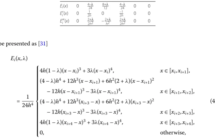
Table 1 Coefficients of extended cubic basisEi(x) and its derivatives at different knots
be presented as [31]
Ei(x,λ) basis and cubic B-spline possess the same properties. When λ= 0 it should be stated that the ExCuBs basis functions will be transformed into cubic B-spline basis. The spline {E0,E0, . . . ,EN+1}forms a basis over the considered domain [a,b]. Coefficients of ExCuBs and its derivatives at different knots are given in Table1.
3 Time discretization
The Caputo fractional derivative is employed to discretize the time of the given problem. Supposetn=nτ,n= 0, 1, . . . ,Min whichτ=MT is the time step size. Forward finite
dif-ference technique is utilized for the discretization of Caputo fractional derivative. The Caputo derivatives ∂α∂ut(αx,t),
∂2αu(x,t)
∂t2α of problem statement can be described as
∂αu(x,t)
The discretized form of the Caputo derivative using a first order forward finite difference method [32] can be written as follows:
∂α(x,t
Discretization of the Caputo derivative using a second order forward finite difference method [16] can be written as
∂2α(x,tn+1) ∂t2α =
1 Γ(3 – 2α)
n
j=0
u(x,tn–j+1) – 2u(x,tn–j) +u(x,tn–j–1) τ2α
×(j+ 1)2–2α–j2–2α+rnτ+1.
The above equation can be rewritten as
∂2α(x,t
n+1) ∂t2α =
1 Γ(3 – 2α)
n
j=0
b2jαu(x,tn–j+1) – 2u(x,tn–j) +u(x,tn–j–1)
τ2α
+rnτ+1, (9)
whereb2α
j = (j+ 1)2–2α–j2–2α. The approximation of second order truncation errorrnτ+1 bound is given in [34] as
rnτ+1 ≤Dτ2–α, (10)
whereDis a constant. The following properties of coefficientsbjcan easily be verified [29]: • b0= 1
• b0>b1>b2>· · ·>bj,bj→0asj→ ∞ • bj> 0forj= 0, 1, . . . ,n
• nj=0(bj–bj+1) +bj+1= (1 –b1) +ns=1–1(bj–bj+1) +bn= 1.
Substituting Eqs. (7) and (9) into Eq. (1), we obtain the following form of the time dis-cretization:
β1
n
j=0
b2jαu(x,tn–j+1) – 2u(x,tn–j) +u(x,tn–j–1)
+β2
n
j=0
bαju(x,tn–j+1)
–u(x,tn–j)
+μux,tn+1=ν∂
2u(x,tn+1) ∂x2 +f
x,tn+1
whereβ1=τ2αΓ1(3–2α)andβ2=ταΓ2(2–λ α).
Supposeun+1=u(x,tn+1) andfn+1=f(x,tn+1), the above equation can be rewritten as
β1
un+1– 2un+un–1+β2
un+1–un+β1
n
j=1
b2jαun+1–j– 2un–j
+un–j–1+β2
n
j=1
bαjun+1–j–un–j+μun+1=ν∂ 2un+1 ∂x2 +f
n+1 (11)
wheren= 0, 1, . . . ,M. It is noticed thatu–1will appear forj= 0,n. The initial velocity condi-tion is used to calculate this term via a central difference formula. We obtain the following result:
4 Description of technique
The approximated solution U(x,t) of given model using ExCuBs to the exact solution
u(x,t) is described in the following form [35,36]:
U(x,t) =
N+1
i=–1
di(t)Ei(x,λ), (13)
wheredi(t) are the time dependent unknown coefficients which are to be required by some
particular restrictions. Each subinterval [xi,xi+1] of basis function covers only three non-zero elementsEi–1,Ei,Ei+1. The approximated solutionunj at the grid point (xj,tn) at the
nth time level to the exact solution is defined as
unj =
i+1
j=i–1
dnj(t)Ej(x,λ),
wherei= 0, 1, . . . ,N. Using the above approximation and basis functions, the valuesunj and their necessary derivatives up to second order as given below:
uni =c1din–1+c2dni +c1din+1, (ux)ni =c3dni+1–c3dni–1, (uxx)ni =c4dni–1–c5din+c4dni+1,
wherec1=4–24λ,c2=8+12λ,c3=21h,c4=2+2h2λ,c5=2+h2λ.
The Caputo derivatives and ExCuBs are used to discretize the model problem. Using the approximation and its derivatives in Eq. (11) and after simplification we obtain the recurrence relation in the following form:
(β1+β2+μ)c1–νc4
dnj–1+1+(β1+β2+μ)c2–νc5
djn+1+(β1+β2+μ)c1–νc4
dnj+1+1
= ⎧ ⎪ ⎪ ⎪ ⎪ ⎪ ⎨ ⎪ ⎪ ⎪ ⎪ ⎪ ⎩
(2β1+β2)(c1djn–1+c2djn+c1djn+1) –β1(c1dnj–1–1+c2dnj–1+c1djn+1–1) –β1
n
k=1b2kα[c1(dnj–1+1–k– 2djn–1–k+dnj–1–1–k) +c2(dnj+1–k– 2dnj–k
+dn–1–k
j ) +c1(djn+1+1–k– 2dnj+1–k+dnj+1–1–k)] –β2nk=1bαk[c1(dnj–1+1–k –djn–1–k) +c2(djn+1–k–dnj–k) +c1(dnj+1+1–k–djn+1–k)] +fjn+1.
(14)
The above system carries (N+ 1)×(N+ 3) dimensions. To solve the above system for unique solution we need two additional equations which will come from boundary con-ditions. Thus the system has (N+ 3)×(N+ 3) dimensions.
5 Initial case
In order to start the iterative process, it is necessary to find the initial vector d0 = [d0
0,d01, . . . ,d0N] which can be evaluated from initial conditions. We employ the initial
con-dition with its derivatives explained below:
(i) dxd(u0
Hence we obtain a systemAu=b, whereAis the matrix of dimension (N+ 3)×(N+ 3) which can be written as
A=
In this section, we use the Von Neumann stability analysis to investigate the stability of proposed scheme. Consider the growth factor in the form of a one Fourier mode as
Ujn=ξneiwhj, (15)
with no forcing term. Herei=√–1,wandhare the mode number and the element size, respectively. We have
The above equation shows a round off error equation. Consider Eq. (15) to be the solution, then the above equation becomes
–β2
Throughout dividing byeiwhjand rearranging the terms, we obtain
After some calculation, we get the following equality:
ξn+1= 1
whereα1is a positive constant.
Proof We prove this proposition with the help of mathematical induction. Forn= 0, in Eq. (16), we get the following relation:
≤ 1 ω(1 +α1)
2 ξ0 –α1(1 +α1) ω ξ
0 –α1(1 +α1) ω
n
k=1
b2kα ξ0
– 2 ξ0 + ξ0 –α2(1 +α1) ω
n
k=1
bαk ξ0 – ξ0 ≤(1 +α1)[1 +α1–α1] ξ0 ,
ξn+1 ≤(1 +α1) ξ0 .
Thus|ξn+1|=|Ujn+1| ≤(1 +α1)|ξ0|= (1 +α1)|Uj0|, so thatUjn+12≤(1 +α1)ξ02. Thus one concludes that the proposed numerical scheme is unconditionally stable.
7 Convergence
In this part, we will investigate the convergence of proposed technique using the Lopez-Marcos [37] method, which plays a significant role in the theory of convergence analysis of fractional type equation. Here we take a few results and notations from [37]. Assume that Ωx={xj; 0≤j≤N}andΩt={tn; 0≤n≤M}be the equidistant partitioning of intervals
[a,b] and [0,T] with the step sizehandτ, respectively. Considerun
j be the approximated
solution at the grid point (xj,tn) andV={vj; 0≤j≤N},W={wj; 0≤j≤N}be the two
functions defined onΩx. We define difference notation as follows:
δ2V=vj+1– 2vj+vj–1, δV=vj+1–vj
V2= (V,V), (V,W) =
N
j=1
hvjwj,
(Vxx,V) = –(Vx,Vx), (V,Wx) = –(Vx,W).
We also suppose thatutt,uxxxxare continuous over the intervals [a,b] and [0,T], and that
there is a positive constantF, such that
|utt| ≤F, |uxxxx| ≤F. (18)
The above values are different at different locations and independent ofj,n,h,τ and for (x,t)∈Ωx×Ωt.
Proposition 7.1([37]) Let{z0,z1, . . . ,zn, . . .}be a monotonically decreasing sequence with
the properties zn≥0and zn+1+zn–1≥2zn.Then,for any positive integer S and for each
vector(v1,v2, . . . ,vS)with S real entries,we have S–1
n=0
n
m=0
zmVn+1–m
Vn+1≥0. (19)
So for the proposed scheme, we have
β1
n
j=0
b2α
j
u(x,tn–j+1) – 2u(x,tn–j) +u(x,tn–j–1)
+β2
n
j=0
bα
j
u(x,tn–j+1)
–u(x,tn–j)
+μux,tn+1=ν∂
2u(x,tn+1) ∂x2 +f
and
j be the solutions of given model and Eq. (20),
re-spectively,and u(x,t)satisfies the smoothness condition(18),then we have
En+1≤Oτ2–α+h2, (22)
where Enj+1=u(xj,tn+1) –unj+1,for every t≥0and suitably small h andτ.
Proof Subtract Eq. (20) from Eq. (21), we get the error equation as follows:
β1
j on both sides of the above equation
and sum up the terms for j, which varies from 1 toN, we obtain
After repositioning the terms, we obtain
Sinceμ1(En+1)
The remaining terms are
En2+β1
Taking the sum of all the above inequalities, we have
n
By Proposition7.1, we can deduce that
β1
Therefore Eq. (23) can be written as
Using the Cauchy–Schwarz inequality, we get
En+12≤ 1
μ
pk+1,Ek+1≤ 1
μp
k+1Ek+1.
From the above inequality, we can get the desired result,
En+1≤Oτ2–α+h2.
8 Numerical examples and discussions
In this section, some numerical experiments are discussed to demonstrate the feasibility of the proposed method. The calculated error norms are established by absoluteL∞and EuclideanL2norms, i.e.,
L∞=U(xi,t) –u(xi,t)∞= max
0≤i≤N
u(xi,t) –u(xi,t) ,
L2=U(xi,t) –u(xi,t)2=
hN
i=0
u(xi,t) –u(xi,t) 2.
The following formula can be used to calculate the order of convergence [38] numeri-cally:
Order =log(L
∞(N
i)) –log(L∞(Ni+1))
log(Ni+1) –log(Ni)
,
whereL∞(Ni) andL∞(Ni+1) are the absolute errors at number of partitioningNiandNi+1, respectively.
Problem 1 Consider the TFTE of the form
∂2αu(x,t) ∂t2α +
∂αu(x,t) ∂tα =
∂2u(x,t)
∂x2 +f(x,t), (24)
wheref(x,t) is suitable with the exact solutionu(x,t) =t2+αsin(2πx) [16], for all (x,t)∈ [0, 1]×[0, 1], where the initial and boundary conditions are
⎧ ⎪ ⎪ ⎪ ⎪ ⎪ ⎨ ⎪ ⎪ ⎪ ⎪ ⎪ ⎩
f1(x) = 0,
f2(x) = 0,
g1(t) = 0,
g2(t) = 0.
(25)
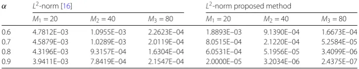
In Table2, we calculate theL2-norm for different spatial and temporal step sizeh= 5, τ = 1
M, (M= 20, 40, 80). In Table3, we determine the order of convergence [16,29] from the
maxi-Table 2 A comparison ofL2norm withh= 5τ=M1 atT= 1 for Problem1
α L2-norm [16] L2-norm proposed method
M1= 20 M2= 40 M3= 80 M1= 20 M2= 40 M3= 80
0.6 4.7812E–03 1.0955E–03 2.2623E–04 1.8893E–03 9.1390E–04 1.6673E–04 0.7 4.5879E–03 1.0289E–03 2.0119E–04 8.0515E–04 2.1220E–04 5.2584E–05 0.8 4.3196E–03 9.3157E–04 1.6304E–04 6.0531E–04 5.1956E–05 3.4099E–06 0.9 3.9411E–03 7.8419E–04 2.1547E–04 2.0000E–05 3.2034E–06 2.4375E–07
Table 3 A comparison of maximum error withh= 5τ=M1 atT= 1 for Problem1
α L∞-norm proposed method
M1= 20 M2= 40 M3= 80 Order= (MM1
2) Order= (
M2 M3)
0.6 2.6719E–03 1.2925E–03 2.3579E–04 1.04776 2.45455
0.7 1.1387E–03 3.0010E–04 7.4366E–05 1.92380 2.01273
0.8 8.5604E–04 7.3478E–05 4.8224E–06 3.54230 3.92949
0.9 2.8285E–05 4.5303E–06 3.4471E–07 2.64239 3.71615
Table 4 Maximum absolute errors and Euclidean norm (L2) for Problem1
N Proposed method
L∞-norm L2-norm Order of convergence CPU time
05 4.5584E–04 3.3892E–04 . . . 0.234002
10 9.1361E–05 6.7926E–05 2.31889 0.249602
20 1.5847E–05 1.1206E–05 2.52731 0.265202
40 9.2497E–07 6.5406E–07 4.09870 0.624004
mum absolute error, the Euclidean norm, the order of convergence and the CPU time for α= 0.75 andτ=1001 .
Problem 2 Consider the TFTE withλ=12,μ= 0 andν=12:
∂2αu(x,t) ∂t2α +
∂αu(x,t) ∂tα =
1 2
∂2u(x,t)
∂x2 +f(x,t) (26)
having the initial condition and boundary conditions
⎧ ⎪ ⎪ ⎪ ⎪ ⎪ ⎨ ⎪ ⎪ ⎪ ⎪ ⎪ ⎩
f1(x) = 0,
f2(x) = 0,
g1(t) =t2,
g2(t) =et2,
(27)
wheref(x,t) is appropriate for the exact solutionu(x,t) =t2ex[39] with 0≤t≤1, 0≤x≤1
and 0 <α< 1.
The comparisons of maximum absolute errors are demonstrated in Table 5for α= 0.64, 0.80, 0.96. Here we choose step sizesh=N1 andτ=N12 forN= 4, 8, 12. TheL2-norm
Table 5 A comparison of maximum absolute error withh=1N,τ= 1
N2 atT= 1 for Problem2
α L∞-norm [39] L∞-norm proposed method
N1= 4 N2= 8 N3= 12 N1= 4 N2= 8 N3= 12
0.64 1.8691E–03 2.4918E–04 7.7737E–05 7.1339E–04 4.7992E–05 2.0457E–05 0.80 2.6820E–03 5.8744E–04 5.6021E–05 9.1889E–04 2.1762E–04 8.4597E–05 0.96 2.3345E–03 4.9965E–04 2.1047E–04 3.4711E–03 9.9307E–04 4.2965E–04
Table 6 A comparison ofL2-norm withh=N1,τ= 1
N2 atT= 1 for Problem2
α L2-norm proposed method
N1= 4 N2= 8 N3= 12 Order= (NN1
2) Order= (
N2 N3)
0.64 4.6716E–04 2.5236E–05 1.2218E–05 3.89381 1.23020
0.80 6.6620E–04 1.4635E–04 5.6375E–05 2.07811 1.36311
0.96 2.5837E–03 6.6449E–04 2.8156E–04 1.80541 1.20875
Table 7 Maximum absolute errors and Euclidean norm (L2) atT= 1 for Problem2
N Proposed method
L∞-norm L2-norm Order of convergence CPU time
05 8.8698E–04 6.1072E–04 . . . 0.010000
10 8.4295E–05 5.1641E–05 3.395390 0.156001
20 1.6730E–05 9.3427E–06 2.332970 5.366430
40 2.7584E–06 1.5267E–06 2.600560 189.6500
Figure 1Comparison plots of exact solutions and approximated solutions for Problem1and Problem2, respectively
Figure 2Error plot at different time level for Problem1and Problem2, respectively
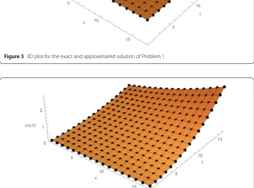
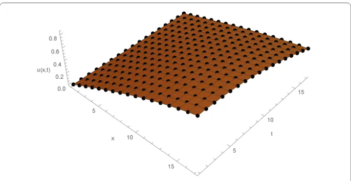
Figure 33D plot for the exact and approximated solution of Problem1
Figure 43D plot for the exact and approximated solution of Problem2
problems can be visualized in Fig.2. Compatibility of exact and approximated solution for Problem1and Problem2can be viewed in Fig.3and Fig.4, respectively.
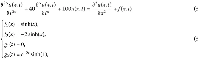
Problem 3 Consider TFTE of the form
∂2αu(x,t) ∂t2α + 20
∂αu(x,t)
∂tα + 25u(x,t) =
∂2u(x,t)
∂x2 +f(x,t) (28)
with the initial and boundary conditions
⎧ ⎪ ⎪ ⎪ ⎪ ⎪ ⎨ ⎪ ⎪ ⎪ ⎪ ⎪ ⎩
f1(x) =sin(x),
f2(x) = 0,
g1(t) = 0,
g2(t) =cos(t)sin(1),
Table 8 A comparison of maximum absolute errors atT= 0.5 for Problem3
x Collocation method [1] Proposed method
α= 0.925 α= 0.975 α= 0.925 α= 0.975
0.0 8.674E–19 1.735E–18 4.718E–16 1.296E–14
0.1 1.571E–03 5.550E–04 4.478E–05 1.213E–05
0.2 2.712E–03 9.255E–04 9.144E–05 2.431E–05
0.3 3.736E–03 1.242E–03 1.317E–04 3.601E–05
0.4 4.782E–03 1.580E–03 1.775E–04 4.694E–05
0.5 5.829E–03 1.921E–03 2.240E–04 5.926E–05
0.6 6.702E–03 2.208E–03 2.357E–04 7.234E–05
0.7 7.080E–03 2.330E–03 3.064E–04 7.153E–05
0.8 6.503E–03 2.132E–03 4.151E–04 3.442E–05
0.9 4.382E–03 1.428E–03 3.649E–05 2.507E–05
1.0 8.882E–16 2.109E–15 2.220E–16 1.110E–16
Table 9 TheL∞-norm andL2-norm withh= 10τ=M1 atT= 0.5 for Problem3
M L∞-norm L2-norm Order of convergence CPU time
10 6.3945E–03 4.1790E–03 . . . 0.046800
20 2.8520E–03 1.7969E–03 1.16485 0.218401
40 1.4143E–03 8.1901E–04 1.01187 1.419609
80 6.6496E–04 1.2428E–04 1.08877 25.31896
wheref(x,t) = –20sin(x)sin(t) + 25sin(x)cos(t) is relevant with the exact solutionu(x,t) =
sin(x)cos(t) [1], 0≤t≤1, 0≤x≤1 and 0 <α< 1.
In Table8, we present a comparison of maximum absolute errors atT = 0.5, forα= 0.925, 0.975 with the results given by Asgariet al.[1]. In Table9, we selecth= 10τ=M1 atT= 0.5 forα= 0.9 and present maximum norm, Euclidean norm and order of conver-gence.
Problem 4 Consider TFTE of the form
∂2αu(x,t) ∂t2α + 40
∂αu(x,t)
∂tα + 100u(x,t) =
∂2u(x,t)
∂x2 +f(x,t) (30)
⎧ ⎪ ⎪ ⎪ ⎪ ⎪ ⎨ ⎪ ⎪ ⎪ ⎪ ⎪ ⎩
f1(x) =sinh(x),
f2(x) = –2sinh(x),
g1(t) = 0,
g2(t) =e–2tsinh(1),
(31)
where f(x,t) = 23e–2tsinh(x) is the appropriate forcing term with the exact solution
u(x,t) =e–2tsinh(x) [1], 0≤t≤1, 0≤x≤1 and 0 <α< 1.
Table10shows the maximum absolute errors of knots for timeT= 0.5,α= 0.975 and
Table 10 A comparison of maximum absolute errors atT= 0.5 for Problem4
x Collocation method [1] Proposed method
n= 3 n= 4 n= 5
0.0 4.426E–04 8.630E–05 2.150E–06 2.124E–13
0.1 7.578E–05 6.734E–05 2.965E–05 9.291E–06
0.2 2.117E–05 1.172E–04 2.082E–04 1.880E–05
0.3 5.044E–04 1.851E–05 3.804E–04 2.786E–05
0.4 3.169E–04 3.180E–04 2.702E–04 3.722E–05
0.5 1.368E–03 1.011E–03 3.151E–04 5.587E–05
0.6 2.990E–03 1.997E–03 1.499E–03 7.070E–05
0.7 2.689E–03 3.270E–03 3.168E–03 7.080E–05
0.8 3.304E–02 6.917E–03 4.472E–03 7.028E–04
0.9 1.212E–01 2.302E–02 2.676E–03 1.692E–03
Table 11 TheL∞-norm andL2-norm withh= 2τ= 1
MatT= 0.5 for Problem4
M L∞-norm L2-norm Order of convergence CPU time
05 3.6153E–02 1.7707E–02 . . . 0.000010
10 1.0277E–02 5.3252E–03 1.81466 0.000013
20 2.3389E–03 5.8122E–04 2.13554 0.015600
40 9.2184E–04 5.8122E–04 1.34324 0.078000
Figure 5Error plot at different time level for Problem3and Problem4respectively
It is simple to notice that convergence rate obtained by the present method is compatible with the theoretical results. The proposed method needs a small storage and less CPU time, which shows the simplicity and strength of the proposed scheme. It is concluded that the present scheme has a great capacity to deal with the fractional order partial differential equations.
9 Conclusion
Figure 63D plot for the exact and approximated solution of Problem3
Figure 73D plot for the exact and approximated solution of Problem4
Acknowledgements
The authors are grateful to the anonymous reviewers for their helpful, valuable comments and suggestions in the improvement of this manuscript. The authors also gratefully acknowledge that this research was financially supported by School of Mathematical Sciences, Universiti Sains Malaysia.
Funding Not applicable.
Availability of data and materials Not applicable.
Competing interests
The authors declare that they have no competing interests.
Authors’ contributions
All authors contributed equally to this work. All authors read and approved the final manuscript.
Author details
Publisher’s Note
Springer Nature remains neutral with regard to jurisdictional claims in published maps and institutional affiliations.
Received: 11 February 2019 Accepted: 13 August 2019 References
1. Asgari, M., Ezzati, R., Allahviranloo, T.: Numerical solution of time fractional order telegraph equation by Bernstein polynomials operational matrices. Math. Probl. Eng.2016, Article ID 1683849 (2016)
2. Hashemi, M.S., Baleanu, D.: Numerical approximation of higher order time fractional telegraph equation by using a combination of a geometric approach and method of line. J. Comput. Phys.316, 10–20 (2016)
3. Diethelm, K., Freed, A.D.: On solution of nonlinear fractional order differential equations used in modelling of viscoplasticity. In: Scientific Computing in Chemical Engineering II. Computational Fluid Dynamics, Reaction Engineering and Molecular Properties, pp. 217–224. Springer, Heidelberg (1999)
4. Kilbas, A.A., Srivastava, H.M., Trujillo, J.J.: Theory and Applications of Fractional Differential Equations. Elsevier, San Diego (2006)
5. Machado, J.A.T.: A probabilistic interpretation of the fractional-order differentiation. Fract. Calc. Appl. Anal.6, 73–80 (2003)
6. Weston, V.H., He, S.: Wave splitting of the telegraph equation inR3and its application to inverse scattering. Inverse Probl.9(6), 789–812 (1993)
7. Jordan, P.M., Puri, A.: Digital signal propagation in dispersive media. J. Appl. Philos.85(3), 1273–1282 (1999) 8. Banasiak, J., Mika, J.R.: Singular perturbed telegraph equations with applications in the random walk theory. J. Appl.
Math. Stoch. Anal.11(1), 9–28 (1998)
9. Saadatmandi, A., Dehghan, M.: Numerical solution of hyperbolic telegraph equation using the Chebyshev tau method. Numer. Methods Partial Differ. Equ.26(1), 239–252 (2010)
10. Cascaval, R.C., Eckstein, E.C., Frota, C.L., Goldstein, J.A.: Fractional telegraph equations. J. Math. Anal. Appl.276(1), 145–159 (2002)
11. Chen, J., Liu, F., Anh, V.: Analytical solution for the time fractional telegraph equation by the method of separating variables. J. Math. Anal. Appl.338(2), 1364–1377 (2008)
12. Momani, S.: Analytic and approximate solutions of the space and time-fractional telegraph equations. Appl. Math. Comput.170(2), 1126–1134 (2005)
13. Huang, F.: Analytical solution for the time-fractional telegraph equation. J. Appl. Math.2009, Article ID 890158 (2009) 14. Dehghan, M., Shokri, A.: A numerical method for solving the hyperbolic telegraph equation. Numer. Methods Partial
Differ. Equ.24(4), 1080–1093 (2008)
15. Yousefi, S.A.: Legendre multiwavelet Galerkin method for solving the hyperbolic telegraph equation. Numer. Methods Partial Differ. Equ.26(3), 535–543 (2010)
16. Wang, J., Zhao, M., Zhang, M., Liu, Y., Li, H.: Numerical analysis of anH1-Galerkin mixed finite element method for time fractional telegraph equation. Sci. World J.2014, Article ID 371413 (2014)
17. Li, C., Cao, J.: A finite difference method for time fractional telegraph equation, mechatronics and embedded sys. In: Appl. (MESA), IEEE/ASME International Conference on, pp. 314–318. IEEE, New York (2012)
18. Saadatmandi, A., Mohabbati, M.: Numerical solutions of fractional telegraph equation via the tau method. Math. Rep. 17(67)(2), 155–166 (2015)
19. Alkahtani, B.S., Gulati, V., Goswami, P.: On the solution of generalized space time fractional telegraph equation. Math. Probl. Eng.2015, Article ID 861073 (2015)
20. Wang, Y.L., Du, M.J., Temuer, C.L., Tian, D.: Using reproducing kernel for solving a class of time fractional telegraph equation with initial value conditions. Int. J. Comput. Math. (2017)
21. Wang, Y., Mei, L.: Generalized finite difference/spectral Galerkin approximations for the time fractional telegraph equation. Adv. Differ. Equ.2017, 281 (2017)
22. Liu, R.: Fractional difference approximations for time fractional telegraph equation. Z. Angew. Math. Phys.6, 301–309 (2018)
23. Tasbozan, O., Esen, A., Yagmurlu, N.M., Ucar, Y.: A numerical solution to fractional diffusion equation for force-free case. Abstr. Appl. Anal.2013, Article ID 187383 (2013)
24. Akram, G., Tariq, H.: Quintic spline collocation method for fractional boundary value problems. J. Assoc. Arab Univ. Basic Appl. Sci. (2016)
25. Sayevand, K., Yazdani, A., Arjang, F.: Cubic B-spline collocation method and its application for anomalous fractional diffusion equations in transport dynamic systems. J. Vib. Control22(9), 2173–2186 (2016)
26. Arshed, S.: Quintic B-spline method for time-fractional superdiffusion fourth-order differential equation. Math. Sci.11, 17–26 (2017)
27. Tasbozan, O., Esen, A.: Quadratic B-spline Galerkin method for numerical solutions of fractional telegraph equations. Bull. Math. Sci. Appl.18, 23–39 (2017)
28. Yaseen, M., Abbas, M., Nazir, T., Baleanu, D.: A finite difference scheme based on cubic trigonometric B-splines for time fractional diffusion-wave equation. Adv. Differ. Equ.2017, 274 (2017)
29. Mohyud-Din, S.T., Akram, T., Abbas, M., Ismail, A.I., Ali, N.H.: A fully implicit finite difference scheme based on extended cubic B-splines for time fractional advection–diffusion equation. Adv. Differ. Equ.2018, 109 (2018)
30. Caputo, M.: Elasticita e Dissipazione. Zanichelli, Bologna, Italy (1969)
31. Han, X.L., Liu, S.J.: An extension of the cubic uniform B-spline curves. J. Comput.-Aided Des. Comput. Graph.15(5), 576–578 (2003)
32. Liu, F., Zhuang, P., Anh, V.: Stability and convergence of the difference methods for the space-time fractional advection-diffusion equation. Appl. Math. Comput.191, 12–20 (2007)
33. Lin, Y., Xu, C.: Finite difference/spectral approximations for the time fractional diffusion equation. J. Comput. Phys. 225, 1533–1552 (2007)
35. Prenter, P.M.: Splines and Variational Methods. Wiley, New York (1989) 36. Boor, C.D.: A Practical Guide to Splines. Springer, Berlin (1978)
37. Marcos, J.C.L.: A difference scheme for a nonlinear partial integro differential equation. SIAM J. Numer. Anal.27(1), 20–31 (1990)
38. Abbas, M., Majid, A.A., Ismail, A.I., Rashid, A.: The application of cubic trigonometric B-spline to the numerical solution of the hyperbolic problems. Appl. Math. Comput.239, 74–88 (2014)