Stability analysis of a certain class of difference equations by using KAM theory

(1)

R E S E A R C H

Open Access

Stability analysis of a certain class of

difference equations by using KAM theory

Senada Kalabuši´c

1*

_{, Emin Bešo}

1

_{, Naida Muji´c}

2

_{and Esmir Pilav}

1

*_{Correspondence:}

[email protected] 1_{Department of Mathematics,} Faculty of Science, University of Sarajevo, Sarajevo, Bosnia and Herzegovina

Full list of author information is available at the end of the article

Abstract

By using KAM theory we investigate the stability of equilibrium points of the class of diﬀerence equations of the formxn+1=f_x(_nx_–1n),n= 0, 1,. . .,f: (0, +∞)→(0, +∞),fis

suﬃciently smooth and the initial conditions arex–1,x0∈(0, +∞). We establish when

an elliptic fixed point of the associated map is non-resonant and non-degenerate, and we compute the first twist coefficient

α

1. Then we apply the results to several

diﬀerence equations.

Keywords: Area-preserving map; Diﬀerence equation; KAM theory; Periodic orbit

1 Introduction and preliminaries

By using KAM (Kolmogorov–Arnold–Mozer) theory we investigate the stability proper-ties of solutions of the following class of second-order diﬀerence equations:

xn+1=

f(xn)

xn–1

, n= 0, 1, . . . , (1)

where f is suﬃciently smooth, f : (0, +∞)→ (0, +∞), and the initial conditions are

x–1,x0∈(0, +∞).

Equation (1) is considered in the book [18] wheref : (0, +∞)→(0, +∞) and the

ini-tial conditions arex–1,x0∈(0, +∞). In particular, several open problems and conjectures

concerning the possible choice of the functionf, for which the diﬀerence equation (1) is

globally periodic, are listed. In [25] the answers to some open problems and conjectures

listed in the book [18] are given. Precisely, for the casesp≤5, necessary and suﬃcient

conditions onf for all solutions to be periodic with periodpare found.

The well-known diﬀerence equation of the form (1) is Lyness’ equation

xn+1=

xn+β

xn–1

, n= 0, 1, . . . . (2)

Several authors have studied the Lyness equation (2) and have obtained numerous results

concerning the stability of equilibrium, non-existence of solutions that converge to the

equilibrium point, the existence of invariants, etc.; see [2,14,15,17,19,35]. See [16] for

the application of the KAM theory to Lyness equation (2). See also [3,4,6] for the results

on the feasible periods for solutions of (2) and the existence of non-periodic solutions

(2)

of (2). See [20,21] for the results on the stability of Lyness equation (2) with period two and period three coeﬃcients. These proofs were based on the construction of the cor-responding Lyapunov functions associated with the invariants of the equation. See also

[21] for the results on the stability of Lyness equation with period two coeﬃcient by using

KAM theory.

In [1,7] authors consider the rational second-order diﬀerence equation

xn+1= α

(1 +xn)xn–1

, n= 0, 1, 2, . . . , (3)

as a special case of the rational diﬀerence equation

xn+1=

α+βxnxn–1+γxn–1

A+Bxnxn–1+Cxn–1

, n= 0, 1, 2, . . . ,

with nonnegative parameters and with arbitrary nonnegative initial conditions such that

the denominator is always positive. Equation (3) is of the form (1). Equation (3) possesses

the following invariant:

xn–1+xn+xn–1xn+α

1 xn–1

+ 1

xn

= constant, ∀n≥0.

See [1]. Equation (3) has a unique positive equilibrium point, and the characteristic

equa-tion of the linearized equaequa-tion of (3) about the equilibrium point has two complex

con-jugate roots on|λ|= 1. Several conjectures and open problems concerning the stability of

the equilibrium point as well as the periodicity of solutions are listed, see [1]. For a more

general case of Equation (3), see [10].

The following equation, which is of the form (1):

yn+1= αy2

n

(1 +yn)yn–1

, n= 1, 2, . . . , (4)

whereαis a parameter, is known as May’s host parasitoid equation, see [22]. In [22] the

authors investigated the corresponding map known as May’s map. More precisely, they investigated the following system of rational diﬀerence equations:

un+1= αun

1 +βvn

,

vn+1= βunvn

1 +βvn

, n= 0, 1, 2, . . . ,

(5)

whereαandβare positive numbers and initial conditionsu0andv0are arbitrary positive

numbers. When α∈(1, +∞) andβ ∈(0,∞) this system is a special case of May’s host

parasitoid model. The change of variablesxn=βunandyn=βvnreduces System (5) to

xn+1= αxn

1 +yn

,

yn+1=

xnyn

1 +yn

, n= 0, 1, 2, . . . .

(3)

By eliminatingxnfrom the right-hand side, System (6) reduces to Equation (4). In [23,24,

33] it was asserted that the positive equilibrium (α

β, α–1

β ) of System (5) is not asymptotically

stable. In [22] it was proved that this is the case, and then, by employing KAM theory, the

authors showed that the positive equilibrium of System (5) is stable. See [30] for results

on periodic solutions.

In [12] authors analyzed a certain class of diﬀerence equations governed by two

param-eters

xn+1=

xk n+a

xpnxn–1

, (7)

wherek,p, andaare positive and the initial conditionsx0,x1are positive. They ﬁxed the

value ofaasa= (2k–p–2_{– 1)/2}k_{and gave an essentially complete description of the global}

behavior of solutions in the ﬁrst quadrant. They showed how Equation (7) leads to

dif-feomorphismF and showed that, for certain parameter value, all suchFshare four key

properties. One of these is thatFhas precisely two ﬁxed points. Then they showed that an

“upper” ﬁxed point is hyperbolic, and they showed by using KAM theory that, by further

restrictingkandl, the origin becomes a neutrally stable elliptic point. Also, they showed

that outside a compact neighborhood of the origin containing the two ﬁxed points, all

points tend to inﬁnity at an exponential rate under the iterates of F andF–1 _{and two}

branches of the eigenmanifolds of the hyperbolic point intersect at a homoclinic point.

Notice that Equation (7) has the form (1).

In [28] authors considered the following diﬀerence equation:

xn+1=

Ax3 n+B

axn–1

, n= 0, 1, . . . , (8)

where the parametersA,B,aand the initial conditionsx–1,x0are positive numbers. They

employed KAM theory to investigate stability property of the positive elliptic equilibrium.

Equation (8) is a special case of the following equation:

xn+1=

Axk_n+B axn–1

, n= 0, 1, . . . .

See [19]. See [13] for the equation

xn+1=

Ax2 n+F

exn–1

, n= 0, 1, . . . .

In [8] authors considered the following diﬀerence equation:

xn+1=

A+Bxn+x2n

(1 +Dxn)xn–1

, n= 0, 1, . . . .

They employed KAM theory to investigate stability property of the positive elliptic equi-librium.

Notice that all of these equations are of the form (1).

By using the methods of algebraic and projective geometry in [4,5], the authors

(4)

global behavior of the following diﬀerence equations:

un+2un=a+bun+1+u2n+1, un+2un=

a+bun+1+cu2n+1

c+un+1

and

un+2un=

a+bun+1+cu2n+1

c+dun+1+u2n+1

.

They obtained very precise description of complicated global behavior which includes ﬁnding the possible periods of all solutions, proving the existence of chaotic solutions through conjugation of maps, and so forth. These methods were ﬁrst used by Zeeman in

[35] for the study of Lyness equation. Notice that each of these equations has the form (1).

Motivated by all these results, we consider any real functionfof one real variable which

is suﬃciently smooth andf : (0, +∞)→(0, +∞), and then we consider Equation (1). In

Sect.2we show how (1) leads to diﬀeomorphismsT andF. We prove some properties

of the mapT, and we establish the condition under which a ﬁxed point (x¯,x¯) of the map

T, in (u,v) coordinates (0, 0), is an elliptic ﬁxed point, wherex¯is an equilibrium point of

Equation (1). In Sect.3we compute the ﬁrst twist coeﬃcientα1, and we establish when an

elliptic ﬁxed point of the mapT is non-resonant and non-degenerate. In Sect.4we apply

our results to several diﬀerence equations of the form (1), and we visualize the behavior

of solutions for some values of the corresponding parameters.

2 Logarithmic coordinate change and area-preserving property

We may write Equation (1) as a mapT: (0, +∞)2_→_{(0, +}_∞₎2_{by setting}

un=xn–1, vn=xn, T

u v

=

v

f(v) u

. (9)

The ﬁxed point (u¯,v¯) of the mapTsatisﬁes the following:

¯

u=v¯ and f(v¯)

¯

u =v¯,

which implies

¯

u2=f(u¯).

Note thatu¯=v¯=x¯, wherex¯is the equilibrium point of Equation (1).

We will assume that all maps are suﬃciently smooth to justify subsequent calculations.

The mapTitself must be diﬀeomorphism of (0, +∞)2_{, and therefore we assume that this}

is the case. The inverse ofT is given by

T–1

u v

=

u

f(u) v

.

The planar mapF isarea-preservingorconservativeif the mapF preserves area of the

planar region under the forward iterate of the map, see [11,19,32]. A diﬀerentiable map

(5)

of the mapFis equal to 1, that is,|detJF(x,y)|= 1 at every point (x,y) of the domain ofF,

see [11,32].

We claim that map (9) is exponentially equivalent to an area-preserving map, see [16].

Let

E(u,v) =xe¯ u,xe¯ vT.

Then

E–1(x,y) =

lnx ¯

x,ln y

¯

x T

,

and if we setF(u,v) =E–1_◦_T_◦_E₍_u_,_v_{), where}_◦_{denotes composition of functions, then we}

obtain a new mappingF, which is given by

F(u,v) =E–1◦T◦E(u,v) =

v

ln(f(ev_x_¯_{)) – 2}_ln₍_x_¯_{) –}_u

.

The mapFis defined on all of R2_{. In fact, since}_T_{was a diffeomorphism of the open first}

quadrantQand sinceEis a diﬀeomorphism of R2_onto_Q_,_F_{is a diﬀeomorphism of R}2

onto itself.

In the study of area-preserving maps, symmetries play an important role since they yield

special dynamic behavior. A transformationRof the plane is said to be a time reversal

symmetry forT ifR–1◦T◦R=T–1, meaning that applying the transformationRto the

mapTis equivalent to iterating the map backwards in time. If the time reversal symmetry

Ris an involution, i.e.,R2=id, then the time reversal symmetry condition is equivalent to

R◦T◦R=T–1_{, and T can be written as the composition of two involutions}_T ₌_I

1◦I0,

withI0=RandI1=T◦R. Note that ifI0=Ris a reversor, then so isI1=T◦R. Also, the

jth involution, deﬁned asIj:=Tj◦R, is also a reversor.

Similar to the proof of Theorem 2.1 in [12], we prove some properties of the mapFin

the following lemma.

Lemma 1 Assume f ∈C1[(0, +∞), (0, +∞)],f(x¯) =x¯2,andx¯> 0,then F shares the following properties:

(a) Fhas the origin as a ﬁxed point; (b) Fis globally area-preserving;

(c) Fsatisfies a time-reversing,mirror image,symmetry condition; (d) All fixed points ofFare located on the diagonal in the first quadrant.

Proof Assertion (a) is immediate. The Jacobian matrix of the mapFis

JF(u,v) =

0 1

–1 evxf_f¯₍_ev(e_x_¯v₎x¯)

, (10)

and sodetJF(u,v) = 1. To explain (c), letR(x,y) = (y,x) which is reﬂection about the

(6)

equation may be rewritten asR◦F=F–1_◦_R_{. For the ﬁnal assertion (d), it is easier to work}

with the original form of our functionT.

A ﬁxed point (x¯,x¯) is anelliptic point of an area-preserving map if the eigenvalues of

JT(x¯,y¯) form a purely imaginary, complex conjugate pairλ,λ¯, see [11,19]. The following

3 The KAM theory and Birkhoff normal form

The stability of an elliptic fixed point of nonlinear area-preserving map cannot be deter-mined solely from linearization, and the effects of the nonlinear terms in local dynamics must be accounted for. This task is facilitated by simplifying the nonlinear terms through appropriate coordinate transformations into Birkhoff normal form.

Consider a smooth, area-preserving map (u,v)→F(u,v) of the plane that has (0, 0) as

an elliptic ﬁxed point, and letλbe an eigenvalue ofJF(0, 0). By putting the linear part of

such a map into Jordan canonical form, by making an appropriate change of variables, we can represent the map in the form

Assume that the eigenvalueλof the elliptic ﬁxed point satisﬁes the non-resonance

condi-tionλk= 1 fork= 1, . . . ,q, for someq≥4. By Lemma 15.37 [11] there exist new canonical

complex coordinates (ζ,ζ¯) relative to which mapping (12) takes the normal form (Birkhoﬀ

normal form)

(7)

in a neighborhood of the elliptic ﬁxed point, whereα(ζζ¯) =α1|ζ|2₊_{· · ·}₊_α

s|ζ|2sis a real

polynomial,s= [q₂] – 1, andgvanishes with its derivatives up to orderq– 1 atζ=ζ¯= 0.

The square brackets denote the largest integer inq/2. The numbersα1, . . . ,αsare called

twist coeﬃcients.

Consider an invariant annulusa<|ζ|<bin a neighborhood of an elliptic ﬁxed point

(0, 0). It is easy to see that the normal form approximationζ→λζeiα(ζζ¯)_{leaves invariant all}

circles|ζ|= const. This map is called a twist mapping. It is easy to describe the dynamics of

the twist map: the orbits are simple rotations on these circles. Also note that if at least one

of the twist coeﬃcientsαjis nonzero, then the angle of rotation is not constant. Applying

KAM-theory (Moser’s twist map theorem [9,27,29,31]) it follows that if a system is close

enough to a twist mapping with rotation angle varying with the radius, then still inﬁnitely

many of the invariant circles survive the perturbation. By [29], p. 245, the rotation angles

of these circles are only badly approximable by rational numbers. According to KAM-theory there exist states close enough to the ﬁxed point, which are enclosed by an invariant curve. Within these gaps, one ﬁnds, in general, orbits of hyperbolic and elliptic periodic points. These facts cannot be deduced from computer pictures. By continuity arguments the interior of such a closed invariant curve will then map onto itself. The same is true for a state within an annulus enclosed between two such curves.

The KAM theorem requires that the elliptic ﬁxed point be resonant and

non-degenerate. Note that, forq= 4, the non-resonance conditionλk= 1 requires thatλ=±1

or±i. The above normal form yields the approximation

ζ →λζ+c1ζ2ζ¯+O

|ζ|4

withc1=iλα1 andα1being the first twist coefficient. We will call an elliptic fixed point

non-degenerate ifα1= 0.

The following is a consequence of Lemma 15.37 [11] and Moser’s twist map theorem [9,

11,27,29].

Theorem 1 Let F:R2_→_R2_{be an area-preserving diﬀeomorphism and}₍_x_,_y₎_{be an elliptic}

ﬁxed point.Assume thatα1= 0.Then there exist periodic points of F with arbitrarily large

period in every neighborhood of(x,y).In addition,ifλ=±1or±i,then the(x,y)is a stable ﬁxed point.

In the sequel we set

f1:=f (x¯), f2:=f (x¯) and f3:=f (x¯).

We prove the following theorem.

Theorem 2 Assume that|f (x¯)|< 2x¯,wherex is an equilibrium point of Equation¯ (1).The elliptic ﬁxed point(0, 0)of the map F,in the(u,v)coordinates,is always non-degenerate. It is non-resonant if and only if

f3=

f2(f2+ 6)x¯4+f1(f2(2f2– 1) + 2)x¯3– 4f12(f2+ 1)x¯2–f13f2x¯+ 2f14 ¯

x3₍_f

1– 2x¯)(x¯+f1)

(8)

Proof To compute the ﬁrst twist coeﬃcientα1, we follow the procedure in [9]. LetFbe

with determinant 1, we change coordinates

(9)

The system in the new coordinates becomes

A tedious symbolic computation done with package Mathematica yields

ξ20=

The above normal form yields the approximation

ζ →λζ+c1ζ2ζ¯+O

|ζ|4

withc1=iλα1andα1being the ﬁrst twist coeﬃcient.

The coeﬃcientc1can be computed directly using the formula

(10)

derived by Wan in the context of Hopf bifurcation theory [34]. In [26] it is shown that when

one uses area-preserving coordinate changes Wan’s formula yields the twist coeﬃcientα1

that is used to verify the non-degeneracy condition necessary to apply the KAM theorem. By using

It can be proved that

α1= –iλ¯c1

Since map (9) is exponentially equivalent to an area-preserving mapF, an immediate

consequence of Theorems1and2is the following result.

Theorem 3 Letx¯> 0be the equilibrium point of (1)such that|f (x¯)|< 2x¯.If (13)holds, then there exist periodic points of T with arbitrarily large period in every neighborhood of (x¯,x¯).In addition,x is a stable equilibrium point of¯ (1).

4 Examples

In this section, we apply Theorem3to several diﬀerence equations of the form (1) that

have been listed in Sect.1.

(11)

wherek,p,aand the initial conditionsx0,x1are positive, is analyzed in [12] with ﬁxed the

value ofaasa= (2k–p–2_{– 1)/2}k_{, where}_k_>_p_{+ 2 and}_p_≥_1.

Now, we assume thatais any positive real number.

The equilibrium point of Equation (16) satisﬁes

¯

xp+2=x¯k+a.

Similar as in Proposition 2.2 [12] one can prove the following.

Proposition 1 Assume that k,p,and a are positive.Let x0be the positive solution of the

equation xk₀–p–2= (p+ 2)/k,and let y0=xp0+2–xk0.Then the following holds:

(a) Ifk>p+ 2,then for0 <a<y0Equation(16)has exactly two positive equilibrium points,fora=y0it has exactly one,and fora>y0it has none.

(b) Ifk<p+ 2,then Equation(16)has exactly one positive equilibrium point.

Since

f (x¯) – 2x¯= –(px¯

k_–_k_x_¯k_{+ 2}_x_¯p+2₊_ap₎ ¯

xp+1

and

f (x¯) + 2x¯= –(px¯

k_–_k_x_¯k_{– 2}_x_¯p+2₊_ap₎ ¯

xp+1 ,

we have that ifx¯> 0 then|f (x¯)|< 2x¯if and only if

(k–p– 2)x¯k<a(p+ 2) and (k–p+ 2)x¯k>a(p– 2). (17)

Hence,x¯is an elliptic point if and only if condition (17) is satisﬁed.

α1=

ak3_x_¯k₍₍_k_–_p_{– 2)(}_k_–_p_{+ 1)}_x_¯2k_{+ 2}_ak_x_¯k_–_a2₍_p2₊_p_{– 2))}

4((–k+p– 2)x¯k₊_a₍_p_{– 2))((–}_k₊_p_{– 1)}_x¯k₊_a₍_p_{– 1))((–}_k₊_p_{+ 2)}_x¯k₊_a₍_p_{+ 2))}2.

Therefore we have the following statement.

Theorem 4 Assume that k,p,and a are positive and the initial conditions x0,x1are

posi-tive.Letx¯> 0be an equilibrium point of (16)and T be the map associated with Equation

(16).Then(x¯,x¯)is an elliptic ﬁxed point of T if and only if

(k–p– 2)x¯k<a(p+ 2) and (k–p+ 2)x¯k>a(p– 2).

Further,if

(k–p– 2)(k–p+ 1)x¯2k+ 2akx¯k–a2p2+p– 2= 0,

(12)

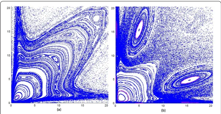
Figure 1Some orbits of the mapTassociated with Eq. (16) for (a)k= 2.1,p= 1, anda= 0.1 and (b)k= 2.01, p= 2, anda= 0.1

Figure1shows phase portraits of the orbits of the mapTassociated with Equation (16)

for some values of the parametersp,k, anda. Neither of these two plots shows any

self-similarity character.

4.2 Example 2:xn+1= A+Bxn+Cxn2 (D+Exn)xn–1

The equation

xn+1=

A+Bxn+Cx2n

(D+Exn)xn–1

, (18)

where A,B,C,D, andE are nonnegative and the initial conditionsx0,x1 are positive, is

analyzed by using the methods of algebraic and projective geometry in [4,5] whereC=D

andE= 1 and by using KAM theory in [8] whereC=D= 1 andA,B,E> 0. Now, we assume

that

(D,E> 0∧A+B> 0)∨(D,E> 0∧A+B= 0∧C>D).

The equilibrium point of Equation (18) satisﬁes

Ex¯3–x¯2(C–D) –Bx¯–A= 0.

By using Descartes’ rule of sign, we obtain that this equation has one positive root.

There-fore, Equation (18) has one positive equilibrium point.

IfD,E> 0, then the changexn=D_Eynconjugates Equation (18) to

yn+1=

a+byn+cy2n

(1 +yn)yn–1

, (19)

where the parametersa,b, andcare

a=AE

2

D3 , b=

BE

D2 and c=

(13)

One can see that the following holds.

Proposition 2 Assume a,b,c≥0and a+b> 0 or a+b= 0∧c> 1.Letx be a positive¯ equilibrium of Equation(19),then|f (x¯)|< 2x¯.

α1=

Γ1+Γ2x¯+Γ3x¯2

2(x¯+ 1)2₍₂_c_x¯₊_x¯₊_b₎₍₂_x¯₍_b_–_c_{+ 1) + (}_c_{+ 2)}_x¯2_{+ 3}_a_–_b₎2₍₂_x¯₍_b₊_c_{+ 1) + (3}_c_{+ 2)}_x¯2₊_a₊_b₎,

where

Γ1=a3b2+ 25a3bc2+ 66a3bc+ 11a3b+ 20a3c3+ 70a3c2+ 55a3c–a3– 2a2b3

– 12a2b2c3+ 5a2b2c2– 8a2b2c– 5a2b2– 29a2bc5– 44a2bc4– 82a2bc3

– 46a2bc2+ 22a2bc+ 2a2b– 8a2c7– 8a2c6– 16a2c5– 2a2c4+ 8a2c2+ 8a2c

+ 3ab4c2+ 8ab4c+ab4+ab3c4+ 16ab3c3– 6ab3c2– 2ab3c– 7ab3– 3ab2c6

+ 10ab2c5– 26ab2c4– 3ab2c3+ab2c2– 5ab2c–ab2–abc8+ 6abc7– 14abc6

+ 8abc5+abc4+ac9– 3ac8+ 3ac7–ac6+b4,

Γ2= 11a3bc+ 4a3b+ 8a3c3+ 63a3c2+ 54a3c+a3+ 24a2b2c2+ 75a2b2c+ 16a2b2

– 20a2bc4– 18a2bc3+ 18a2bc2+ 110a2bc+ 6a2b– 8a2c6– 17a2c5– 33a2c4

– 35a2c3+ 21a2c2+ 37a2c–a2+ab4c–ab4– 10ab3c3+ 18ab3c2–ab3c– 19ab3

– 31ab2c5– 38ab2c4– 95ab2c3– 54ab2c2– 15ab2c– 6ab2– 9abc7– 4abc6

– 25abc5– 3abc4– 4abc2+ 8abc+ab+ac8– 2ac7+ac6+ 3b5c2+ 8b5c+b5

+b4c4+ 16b4c3– 6b4c2– 2b4c–b4– 3b3c6+ 10b3c5– 26b3c4– 3b3c3+b3c2

+ 2b3c–b3–b2c8+ 6b2c7– 14b2c6+ 8b2c5+b2c4+bc9– 3bc8+ 3bc7–bc6,

Γ3= 16a3c2+ 19a3c+a3+ 12a2b2c+ 8a2b2+ 22a2bc3+ 92a2bc2+ 84a2bc+ 6a2b

– 8a2c5– 6a2c4– 10a2c3+ 33a2c2+ 28a2c–a2–ab4+ab3c2+ 15ab3c– 7ab3

– 33ab2c4– 16ab2c3– 65ab2c2– 25ab2c– 6ab2– 38abc6– 30abc5– 78abc4

– 7abc3+ 5abc2+ 9abc+ab– 8ac8+ac7– 9ac6+ 14ac5+ 2ac4+b5c+b5

+ 5b4c3+ 18b4c2–b4–b3c5+ 21b3c4– 35b3c3– 4b3c2+b3c–b3– 4b2c7

+ 17b2c6– 45b2c5+ 22b2c4+ 4b2c3–bc9+ 8bc8– 22bc7+ 23bc6– 7bc5–bc4

+c10– 4c9+ 6c8– 4c7+c6.

In Table1we compute the twist coeﬃcient for some valuesa,b,c≥0.

Theorem 5 Assume that a,b,and c are positive numbers such that a+b> 0.Letx¯> 0be an equilibrium point of Equation(19)and T be the map associated with Equation(19). Then(x¯,x¯)is an elliptic ﬁxed point of T and,ifα1= 0,then there exist periodic points of

(14)

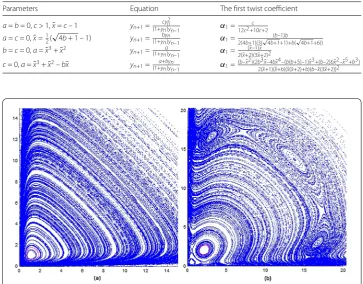
Table 1 The ﬁrst twist coeﬃcient for some values ofa,b,c≥0

Parameters Equation The ﬁrst twist coeﬃcient

a=b= 0,c> 1,¯x=c– 1 yn+1= cy 2 n

(1+yn)_yn_–1 α1=₁₂_c₂₊₁₀c _c₊₂

a=c= 0,x¯=1₂(√4b+ 1 – 1) yn+1=(1+ynbyn)_yn_–1 α1=₂₍₄_b₊₁₎₍₃₍√₄_b(₊₁₊₁₎₊b–1)b_b₍√₄_b₊₁₊₆₎₎ b=c= 0,a=x¯3₊_x_¯2 _yn

+1=₍₁₊_yna₎_yn

–1 α1=

(x¯–1)x¯

2(x¯+2)(3¯x+2)2 c= 0,a=x¯3+x¯2–bx¯ yn+1=₍₁₊a_yn+byn₎_yn

–1 α1=

(b–¯x2)(2b3x¯–4b¯x4–(b(b+5)–1)x¯3+(b–2)bx¯2–¯x5+b3) 2(x¯+1)(¯x+b)(¯x(x¯+2)+b)(b–¯x(3x¯+2))2

Figure 2Some orbits of the mapTassociated with Eq. (19) for (a)a= 0.2,b= 1.05, andc= 1.03 and (b) a= 0.1,b= 0.05, andc= 0.3

for some values of the parametersa,b, andc.

4.3 Example 3:xn+1=a+bxn+cx2n xn–1

In [4,5] the authors analyzed the equation

xn+1=

a+bxn+cx2n

xn–1

, (20)

wherea,b, andcare nonnegative and the initial conditionsx0,x1are positive, by using the

methods of algebraic and projective geometry wherec= 1. It is easy to see that Equation

(20) has one positive equilibrium

¯

x=b+

√

4ac+ 4a+b2

2(1 –c)

forc< 1. Further,|f (x¯)|– 2x¯= –b2_{+ 4}_a_{(1 –}_c_{) < 0.}

By using package Mathematica, we obtain

α1=16a

2₍_c_{– 1)}2_c₍_c_{+ 1) +}_ab2_(–8_c3_{+ 8}_c2₊_c_{– 1) +}_b_Γ 4

√

–4ac+ 4a+b2₊_b4₍_c2_–_c_{+ 1)}

(15)

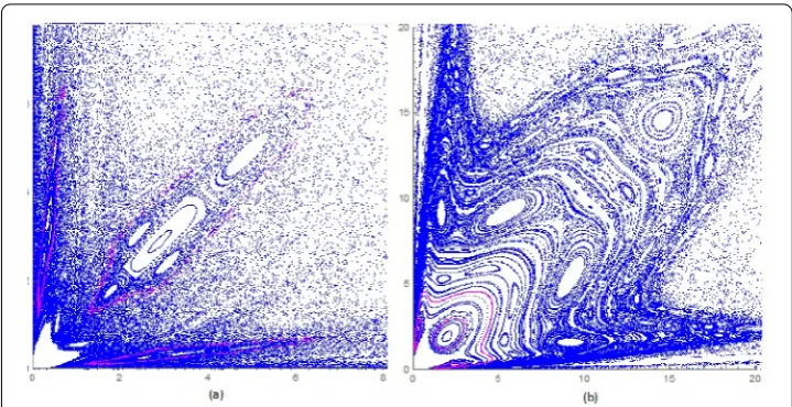
Figure 3Some orbits of the mapTassociated with Eq. (20) for (a)a= 0.1,b= 0.002, andc= 0.001 and (b) a= 0.1,b= 0.02, andc= 0.001

where

Γ4=a

4c3– 12c2+ 7c+ 1–b2c2– 3c+ 1.

Theorem 6 Assume that a,b,and c are positive numbers such that a+b> 0and c< 1.Let

¯

x> 0be the equilibrium point of Equation(20)and T be the map associated with Equation

(20).Then(x¯,x¯)is an elliptic ﬁxed point of T and,ifα1= 0,there exist periodic points with

arbitrarily large period in every neighborhood of(x¯,x¯).In addition,x is a stable equilibrium¯ point of (20).

for some values of the parametersa,b, andc.

5 Conclusion

In this paper, we investigated the stability of a class of diﬀerence equations of the form

xn+1=f_x(_nx_–1n),n= 0, 1, . . . . We assume that the functionfis suﬃciently smooth and the initial

conditions are arbitrary positive real numbers. It is enough to assume that the functionf

is inC(3)_{(0, +}_∞_{). We show how the map}_T_{associated with this diﬀerence equation leads to}

diﬀeomorphismF. We prove some properties of the mapF, and we establish the condition

under which an equilibrium point (0, 0) inu,vcoordinates is an elliptic ﬁxed point. Also,

we compute the first twist coefficient. The condition for an elliptic fixed point to be non-degenerate and non-resonant is established in closed form. This condition depends only

on the values of the ﬁrst, second, and third derivatives of the functionf at the equilibrium

point. We apply our result to several diﬀerence equations that have been investigated by others. By numerical computations, we conﬁrm our analytic results.

Acknowledgements

The authors are thankful to the anonymous referees for their helpful comments and the editor for constructive suggestions to improve the paper in current form.

(16)

Availability of data and materials Not applicable.

Ethics approval and consent to participate Not applicable.

Competing interests

The authors declare that they have no competing interests.

Authors’ contributions

All authors contributed equally and signiﬁcantly in writing this article. All authors read and approved the ﬁnal manuscript.

Author details

1_{Department of Mathematics, Faculty of Science, University of Sarajevo, Sarajevo, Bosnia and Herzegovina.}2_{Faculty of}

Electrical Engineering, University of Sarajevo, Sarajevo, Bosnia and Herzegovina.

Publisher’s Note

Springer Nature remains neutral with regard to jurisdictional claims in published maps and institutional aﬃliations.

Received: 22 March 2019 Accepted: 20 May 2019 References

1. Amleh, A.M., Camouzis, E., Ladas, G.: On the dynamics of a rational diﬀerence equation, part 1. Int. J. Diﬀerence Equ. 3(1), 1–35 (2008)

2. Barbeau, E., Gelbord, B., Tanny, S.: Periodicity of solutions of the generalized Lyness recursion. J. Diﬀer. Equ. Appl.1, 291–306 (1995)

3. Bastien, G., Rogalski, M.: Global behavior of the solutions of Lyness’ diﬀerence equationun+2un=un+1+a. J. Diﬀer.

Equ. Appl.10, 977–1003 (2004)

4. Bastien, G., Rogalski, M.: On some algebraic diﬀerence equationsun+2un=g(un+1) related to families of conics or

cubics: generalization of the Lyness’ sequences. J. Math. Anal. Appl.300, 303–333 (2004)

5. Bastien, G., Rogalski, M.: On the algebraic diﬀerence equationsun+2un=ψ(un+1) inR+∗, related to a family of elliptic

quartics in the plane. Adv. Diﬀer. Equ.2005, 948567 (2005)

6. Beukers, F., Cushman, R.: Zeeman’s monotonicity conjecture. J. Diﬀer. Equ.143, 191–200 (1998)

7. Denette, E., Kulenovi´c, M.R.S., Pilav, E.: Birkhoﬀ normal forms, KAM theory and time reversal symmetry for certain rational map. Mathematics4(1), 20 (2016)

8. Garic-Demirovic, M., Nurkanovic, M., Nurkanovic, Z.: Stability, periodicity, and symmetries of certain second-order fractional diﬀerence equation with quadratic terms via KAM theory. Math. Methods Appl. Sci.40, 306–318 (2017) 9. Gidea, M., Meiss, J.D., Ugarcovici, I., Weiss, H.: Applications of KAM theory to population dynamics. J. Biol. Dyn.5(1),

44–63 (2011)

10. Grove, E.A., Janowski, E.J., Kent, C.M., Ladas, G.: On the rational recursive sequencexn+1=(γxnαxn+δ+)xnβ–1. Commun. Appl.

Nonlinear Anal.1(13), 61–72 (1994)

11. Hale, J.K., Kocak, H.: Dynamics and Bifurcation. Springer, New York (1991)

12. Haymond, R.E., Thomas, E.S.: Phase portraits for a class of difference equations. J. Differ. Equ. Appl.5, 177–202 (1999) 13. Jašarević-Hrustić, S., Kulenović, M.R.S., Nurkanović, Z., Pilav, E.: Birkhoff normal forms, KAM theory and symmetries for

certain second order rational difference equation with quadratic terms. J. Differ. Equ.10(2), 181–199 (2015) 14. Kocic, V.L., Ladas, G.: Global Behavior of Nonlinear Difference Equations of Higher Order with Applications. Kluwer

Academic, Dordreht (1993)

15. Kocic, V.L., Ladas, G., Rodrigues, I.W.: On the rational recursive sequences. J. Math. Anal. Appl.173, 127–157 (1993) 16. Kocic, V.L., Ladas, G., Tzanetopoulos, G., Thomas, E.: On the stability of Lyness equation. In: Dynamics of Continuous,

Discrete and Impulsive Systems (1), pp. 245–254 (1995)

17. Kulenović, M.R.S.: Invariants and related Liapunov functions for difference equations. Appl. Math. Lett.13, 1–8 (2000) 18. Kulenović, M.R.S., Ladas, G.: Dynamics of Second Order Rational Difference Equations: With Open Problems and

Conjectures. Chapman and Hall/CRC, London (2001)

19. Kulenovi´c, M.R.S., Merino, O.: Discrete Dynamical Systems and Diﬀerence Equations with Mathematica. Chapman Hall/CRC, Boca Raton (2002)

20. Kulenović, M.R.S., Nurkanović, Z.: Stability of Lyness equation with period three coefficient. Rad. Mat.12, 153–161 (2004)

21. Kulenović, M.R.S., Nurkanović, Z.: Stability of Lyness equation with period-two coefficient via KAM theory. J. Concr. Appl. Math.6, 229–245 (2008)

22. Ladas, G., Tzanetopoulos, G., Tovbis, A.: On May’s host parasitoid model. J. Diﬀer. Equ. Appl.2, 195–204 (1996) 23. May, R.M.: Host-parasitoid system in patchy environments. A phenomenological model. J. Anim. Ecol.47, 833–843

(1978)

24. May, R.M., Hassel, M.P.: The dynamics of multiparasitoid host interactions. Am. Nat.117, 234–261 (1981) 25. Mestel, B.D.: On globally periodic solutions of the diﬀerence equationxn+1=f_xn(xn_–1). J. Diﬀer. Equ. Appl.3, 201–209

(2001)

26. Moeckel, R.: Generic bifurcations of the twist coeﬃcient. Ergod. Theory Dyn. Syst.10(1), 185–195 (1990) 27. Moser, J.: On invariant curves of area-preserving mappings of an annulus. Nachr. Akad. Wiss. Gött., 21962, 1–20

(1962)

28. Nurkanović, M., Nurkanović, Z.: Birkhoff normal forms, KAM theory, periodicity and symmetries for certain rational difference equation with cubic terms. Sarajevo J. Math.25, 217–231 (2016)

(17)

30. Siezer, W.: Periodicity in the May’s host parasitoid equation. In: Advances Studies in Pure Mathematics 53 (2009) 31. Sternberg, S.: Celestial Mechanics. II. W. A. Benjamin, New York (1969)

32. Tabor, M.: Chaos and Integrability in Nonlinear Dynamics. An Introduction. Wiley, New York (1989)

33. Taylor, A.D.: Aggregation, competition, and host-parasitoid dynamics: stability conditions don’t tell it all. Am. Nat.141, 501–506 (1993)

34. Wan, Y.H.: Computation of the stability condition for the Hopf bifurcationof diﬀeomorphisms onR2_{. SIAM J. Appl.}

Math.34(1), 167–175 (1978)