Turing–Hopf bifurcation of a ratio dependent predator prey model with diffusion

(1)

R E S E A R C H

Open Access

Turing–Hopf bifurcation of a

ratio-dependent predator-prey model with

diffusion

Qiushuang Shi

1

_{, Ming Liu}

1*

_{and Xiaofeng Xu}

1

*_{Correspondence:}

[email protected]

1_{Department of Mathematics,}

Northeast Forestry University, Harbin, P.R. China

Abstract

In this paper, the Turing–Hopf bifurcation of a ratio-dependent predator-prey model with diffusion and Neumann boundary condition is considered. Firstly, we present a kind of double parameters selection method, which can be used to analyze the Turing–Hopf bifurcation of a general reaction-diffusion equation under Neumann boundary condition. By analyzing the distribution of eigenvalues, the stable region, the unstable region (including Turing unstable region), and Turing–Hopf bifurcation point are derived in a double parameters plane. Secondly, by applying this method, the Turing–Hopf bifurcation of a ratio-dependent predator-prey model with diffusion is investigated. Finally, we compute normal forms near Turing–Hopf singularity and verify the theoretical analysis by numerical simulations.

Keywords: Ratio-dependent; Reaction-diﬀusion; Turing–Hopf bifurcation; Predator-prey model

1 Introduction

Due to the existence of rich dynamics, predator-prey systems have received great atten-tion [1–12]. The classical ratio-dependent Holling–Tanner prey-predator model is as fol-lows [13]:

du dt =ru

1 –u k

– auv

mv+u,

dv dt =sv

1 –hv u

.

(1)

Here,uandvis the prey and predator population, respectively,r,s> 0 is the linear birth rate of prey and predator, respectively,k> 0 is the carrying capacity of prey population, h> 0 is the proportionality coeﬃcient of prey density to the carrying capacity for the predator and _mvauv₊_u represents ratio-dependent functional response witha,m> 0, which is signiﬁcant for describing predator consumption of predator-prey models [14–21].

Taking into account the inhomogeneous distribution of the prey and predators in dif-ferent spatial locations and other food sources of predators, model (1) can be modiﬁed as

(2)

follows [22–24]:

∂u

∂t =d1u+u

α1–β1u– γ1v m1v+u

,

∂v

∂t=d2v+v

α2– γ2v m2+u

,

(2)

whereu=u(x,t) andv=v(x,t) is the population density of the prey and predators at loca-tionxand timet, respectively,d1,d2> 0 is the diﬀusion coeﬃcient characterizing the rate of the spatial dispersion of the prey and predator population, respectively.

In this paper, we investigate the Turing–Hopf bifurcation of model (2) with Neumann boundary condition

∂u ∂ν =

∂v

∂ν = 0, x∈∂Ω,t> 0, (3)

whereΩ = (0,lπ) andν is the outward unit normal vector on∂Ω. Because stable spa-tially inhomogeneous periodic solution can be preferably used to explain the periodic fluctuation of biological populations and it is very difficult to obtain stable spatially in-homogeneous periodic solution for research on general Turing or Hopf bifurcation un-der Neumann boundary condition, more and more scholars start to investigate the high codimension bifurcation of reaction-diffusion equation, especially Turing–Hopf bifurca-tion. There exist very rich dynamics near Turing–Hopf singularity, such as stable constant steady state, nonconstant steady state, spatially homogeneous, and inhomogeneous peri-odic solutions.

It is well known that the normal forms theory plays a very important role in the bifur-cation analysis. Faria developed a method to calculate normal forms near an equilibrium of partial functional differential equation [25]. Based on the method of Faria, Song et al. presented a method to compute normal forms near Turing–Hopf singularity of reaction-diffusion equation [26]. However, there are still very few studies on Turing–Hopf bifurca-tion of reacbifurca-tion-diffusion equabifurca-tion with practical significance [27–29].

We would like to mention that one of the most difficult problems for research on Turing– Hopf bifurcation is how to obtain the existence of Turing–Hopf bifurcation. In the previ-ous research, scholars generally chose two appropriate bifurcation parameters such that the Hopf and Turing bifurcation line in a double parameters plane can be defined by a straight line. This method can be easily used to obtain the existence of Turing–Hopf bi-furcation, but it cannot be applied to most reaction-diffusion equations. In this paper, we present a kind of parameter selection method such that the Turing bifurcation line can be defined by a curve, which can be applied to most reaction-diffusion equations.

(3)

2 Existence of Turing–Hopf bifurcation of reaction-diffusion equation

In this section, we consider the Turing–Hopf bifurcation of the following general bivariate reaction-diﬀusion equation:

⎧ ⎪ ⎪ ⎨ ⎪ ⎪ ⎩

∂u(x,t)

∂t =d1u(x,t) +αF(u(x,t),v(x,t)),

∂v(x,t)

∂t =d2v(x,t) +βG(u(x,t),v(x,t)),

x∈Ω,t> 0,

∂u(x,t)

∂ν = ∂v(x,t)

∂ν = 0, x∈∂Ω,t> 0,

(4)

wheref andgare adequately smooth. Moreover, we assume thatα,β> 0 and there exists one positive steady stateE∗(u∗,v∗) of system (4). Takingαandβas bifurcation parameters, we have the characteristic equation at the steady stateE∗as follows:

λ+d1(n_l)2_–_F1(u

∗,v∗)α –F2(u∗,v∗)α –G1(u∗,v∗)β λ+d2(n_l)2–G2(u∗,v∗)β

= 0, n∈N0, (5)

whereN0={0} ∪N. Denote

p11=F1(u∗,v∗), p12=F2(u∗,v∗), p21=G1(u∗,v∗), p22=G2(u∗,v∗),

then Eq. (5) can be written as

n(λ) =λ2+Tnλ+hn= 0, n∈N0, (6)

where

Tn= (d1+d2)

n l

2 +T0,

hn=d1d2

n l

4

+ (–d2p11α–d1p22β)

n l

2 +h0,

(7)

with

T0= –p11α–p22β,

h0= (p11p22–p12p21)αβ.

(8)

For convenience, we denote

D0(α) = – p11

p22α, α> 0, (9)

and make some hypotheses as follows:

(H1) p11p22<p12p21,

(H21) p11p22>p12p21, p11≥0, p22≥0, p2₁₁+p2₂₂= 0,

(H22) p11p22>p12p21, p11≤0, p22≤0, p2₁₁+p2₂₂= 0,

(H23) p11p22>p12p21, p11> 0, p22< 0,

(H24) p11p22>p12p21, p11< 0, p22> 0.

(4)

Lemma 2.1 For system(4)without diﬀusion(d1=d2= 0),we have the following results.

(i) If(H1)or(H21)holds,thenE∗is unstable.

(ii) If(H22)holds,thenE∗is asymptotically stable.

(iii) If(H23)holds,thenE∗is asymptotically stable forβ>D0(α)and unstable for β<D0(α);and the Hopf bifurcation line isβ=D0(α).

(iv) If(H24)holds,thenE∗is asymptotically stable forβ<D0(α)and unstable for

β>D0(α);and the Hopf bifurcation line isβ=D0(α).

Proof Clearly, the characteristic equation forE∗of system (4) without diﬀusion is

0(λ) =λ2+T0λ+h0= 0. (11)

If (H1) holds, then we haveh0< 0. It follows that Eq. (11) has one positive real root and the proof of (i) is completed.

Ifp11p22>p12p21, then we haveh0> 0. Furthermore, we can obtain thatT0< 0 when (H21) holds andT0> 0 when (H22) holds. Thus, the two roots of Eq. (11) have positive real parts when (H21) holds and negative real parts when (H22) holds. The proof of (ii) is completed.

If (H23) holds, we can obtain thath0> 0 andT0< 0 whenβ<D0(α) andT0> 0 whenβ>

D0(α). Moreover,±i√h0are a pair of purely imaginary roots of Eq. (11) whenβ=D0(α) and the transversality condition is as follows:

dRe{λ(α)} dα

β=D0(α)= p11

2 > 0. (12)

Thus,β=D0(α) is the Hopf bifurcation line and the proof of (iii) is completed. We omit

the proof of (iv), because it is similar to the proof of (iii).

Assumptions in (10) do not include the casesp11p22=p12p21andp11=p22= 0, because if p11p22=p12p21holds, one immediately hash0= 0 and 0 is a root of Eq. (11) for anyα,β> 0 and ifp11=p22 = 0 holds, we immediately haveT0= 0 and±i√h0 are a pair of purely imaginary roots of Eq. (11) for anyα,β> 0. Obviously, the double parameters selection method is not eﬀective for these two cases. So we do not discuss them any more in this paper.

Next, we investigate the stability and Turing–Hopf bifurcation of system (4). From the proof of Lemma2.1, we know that Eq. (6) has at least one root with a positive real part for anyα,β> 0 if (H1) or (H21) holds. Moreover, if (H22) holds, one can easily obtain that Tn> 0 andhn> 0 forn∈N0andα,β> 0. Therefore, we have the following result.

Theorem 2.2

(i) If(H1)or(H21)holds,E∗is unstable for anyα,β> 0. (ii) If(H22)holds,E∗is asymptotically stable for anyα,β> 0.

(5)

Ifβ>D0(α) holds, we have thatTn> 0 forn∈N0. And ifhn= 0 holds, we have that

β=Rn(α) =

d2(n_l)2p11α–d1d2(n_l)4 –d1(n_l)2p22+ (p11p22–p12p21)α

, n∈N0. (13)

Obviously, if all lines deﬁned byβ=Rn(α) lie below the Hopf bifurcation lineβ=D0(α),

there is no Turing instability. Note that

D0(α) –Rn(α) =

1

–d1(n_l)2p22+ (p11p22–p12p21)α

Pn(α), (14)

where

Pn(α) = –

p11 p22

(p11p22–p12p21)α2+ (d1–d2)p11

n l

2

α+d1d2

n l

4

. (15)

For convenience, we deﬁne

Λ= (d2–d1)2p2₁₁+ 4d1d2p11

p22(p11p22–p12p21), (16)

and make some hypotheses:

(C1) d2≤d1.

(C2) d2>d1 and Λ< 0.

(C3) d2>d1 and Λ> 0.

(17)

Clearly,D0(α) >Rn(α) is equivalent toPn(α) > 0. Moreover, we can obtain thatPn(α) > 0

forn∈N0if (C1) or (C2) holds. Hence, we have the following result.

Theorem 2.3 Assume that(H23)holds.If(C1)or(C2)is satisfied,then system(4)has no diffusion-driven Turing instability.In this case,diffusion does not change the stability of E∗, i.e.,the stable and unstable regions are the same as those in Lemma2.1(iii).

Then we focus on the case of the existence of Turing instability. It is easy to see that if (C3) holds,D0(α) –Rn(α) = 0,n∈Nhas two positive roots:

A±

n =

–(d1–d2)p11±√Λ –2p11

p22(p11p22–p12p21)

n l

2

(18)

such that

⎧ ⎨ ⎩

D0(α) <Rn(α) ifA–n<α<A+n,

D0(α) >Rn(α) if 0 <α<A–norα>A+n.

For anym,n∈N,m>n, we can obtain that

(6)

= d2(

p11(p11p22–p12p21)l4 (19)

such that with respect tonandB+_(n,_{m) is monotonously increasing with respect to}_m_{for ﬁxed} n∈N.

Moreover, the transversality condition is as follows:

(7)

Otherwise, forΓ0<α≤Γ1=A–2, the boundaries consist ofR1(α) withΓ0<α≤A+1 and

D0(α) withA+

1<α≤Γ1. By using the mathematical induction, we can obtain that all the boundaries of a stable region consist ofTn(α),n∈N0. have negative real parts. Together with the transversality conditions (12) and (18), we have that system (4) undergoes Turing–Hopf bifurcation at (A–1, –pp1122A

n+1), respectively. Meanwhile all other roots, except a pair of purely imaginary roots ±i√h0 of0(λ) = 0, have negative real parts. Thus, (A+n, –pp1122A

From the above analysis, we can detailedly describe the boundary of the unstable region (including Turing unstable region) of the positive steady stateE∗.

Theorem 2.4 Assume that(H23)holds and(C3)is satisﬁed,there exists diﬀusion-driven Turing instability.More precisely,we have the following results.

(i) The boundary of a stable region isβ=Tn(α),n∈N0,and for anyα> 0,β>Tn(α),

n∈N0,the positive steady stateE∗is asymptotically stable.

(ii) For anyα> 0,D0(α) <β<Tn(α),n∈N,there exists Turing instability.

(iii) System(4)undergoes Turing–Hopf bifurcation at the point(A– 1, –

3 Turing–Hopf bifurcation of a diffusive ratio-dependent predator-prey model

Let

then system (2) becomes:

⎧

Next, we use the conclusions of the above section to investigate the stability of positive steady state and Turing–Hopf bifurcation of system (23). With a simple calculation, we have the following result.

Theorem 3.1 Assume that α1,α2,d1,d2,l> 0. Then the existence conditions of positive

steady state of model(23)can be divided into the following three situations: Case A:m1=δand b>hm1m2+ 1.

There exists only one positive steady state E1 = (u1,v1) of model (23) in this case, where

u1=b–hm1m2

h(m1+b) , v1= m2+u1

(8)

Case B:m1>δ.

There exists only one positive steady state E2 = (u2,v2) of model (23) in this case, where

u2=m1+b–hm1m2–δ+c 2h(m1+b)

, v2=m2+u2

b ,

with

c=(m1+b–hm1m2–δ)2_{+ 4hm2(m1}₊_b)(m1_–_δ_).

Case C:m1<δand m1+b–hm1m2–δ> 0.

There exist two positive steady states E3= (u3,v3)and E4= (u4,v4)of model(23)in this case,where

u3=

m1+b–hm1m2–δ–c

2h(m1+b) , v3=

m2+u3

b ,

u4=m1+b–hm1m2–δ+c

2h(m1+b) , v4=

m2+u4

b .

Next,we take the steady state E4as an example to investigate the Turing–Hopf bifurca-tion.Denote

f(u4) =

δm1(m2+u4)2 (m1(m2+u4) +bu4)2,

g(u4) = b

2_u2 4δ

(m1(m2+u4) +bu4)2,

r(u4) = 1 – 2hu4–f(u4).

Then we have

p11=r(u4), p12= –g(u4), p21=1

b, p22= –1.

The characteristic equation at E4is

n(λ) =λ2+Tnλ+hn= 0, n∈N0, (24)

where

Tn= (d1+d2)

n l

2 +T0,

hn=d1d2

n l

4

+d1α2–d2α1r(u4)

n l

2 +h0,

with

T0=α2–α1r(u4),

h0=α1α2 g(u4)

(9)

From the results in Sect.2, one immediately has the following conclusions.

Theorem 3.2

(i) Ifr(u4)≤0holds,the positive steady stateE4of(23)is asymptotically stable for any

α1,α2> 0.

(ii) Ifr(u4) > 0and g(u4)

b <r(u4)hold,the positive steady stateE4of(23)is unstable for anyα1,α2> 0.

Theorem 3.3 Suppose that r(u4) > 0, g(u4)

b >r(u4). If (C1) or (C2) holds, there is no

diﬀusion-driven Turing instability.

Theorem 3.4 Suppose that r(u4) > 0, g(u4)

b >r(u4).If(C3)holds,we have the following

re-sults.

(i) Ifα1> 0,α2>Tn(α1),n∈N0,the steady stateE4is asymptotically stable.

(ii) Turing instability occurs forα1> 0,D0(α1) <α2<Tn(α1),n∈N.

(iii) System(23)undergoes Turing–Hopf bifurcation at(A₁–,r(u4)A–₁);if

A–

n+1>A+n,n∈Nholds,system(23)undergoes Turing–Hopf bifurcation at the point

(A+

n,r(u4)A+n)and(An–+1,r(u4)A–n+1),where

D0(α1) =α1r(u4), α1> 0,

Rn(α1) =

r(u4)α1d2(n_l)2–d1d2(n_l)4

d1(n_l)2₊_α₁₍g(u4)

b –r(u4))

, r> 0,n∈N0.

Λ=r2(u4)(d2–d1)2– 4r(u4)

g(u4) b –r(u4)

d1d2,

A±

n =

r(u4)(d2–d1)±√Λ 2r(u4)(g(u4)

b –r(u4))

n l

2 ,

B+_(n,_{m) =} d1(

g(u4)

b –r(u4)) m2₊_n2

l2 +c1 2r(u4)(g(u_b4)–r(u4))

,

c1= d21

g(u4) b –r(u4)

2

(m2₊_n2₎2

l2 + 4d

2 1r(u4)

g(u4) b –r(u4)

m2_n2 l4 .

ΓnandTnare deﬁned by(21)and(22),respectively,and hypotheses(C1), (C2),and(C3)

are deﬁned by(17).

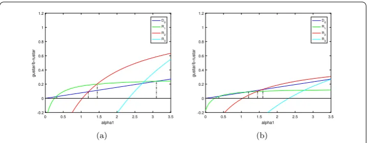
We would like to mention thatA–_n₊₁<A+_nandA–_n₊₁>A+_nare all possible to happen (see Fig.1). Obviously, we haveA–

2<A+1in Fig.1(a) andA–2>A+1in Fig.1(b).

4 Normal forms for Turing–Hopf bifurcation

(10)

Figure 1Bifurcation diagram in the double parameters plane at the positive steady stateE4, where b= 0.35,δ= 0.6,m1= 0.5,m2= 0.3,h= 0.3,l= 1,d1= 0.02. (a):d2= 0.35. (b):d2= 0.17

Letα1=α1∗+μ1andα2=α2∗+μ2, then system (23) becomes

⎧ ⎨ ⎩

∂u

∂t =d1u+ (α1∗+μ1)u(1 –hu–

δv m1v+u),

∂v

∂t =d2v+ (α2∗+μ2)v(1 – bv m2+u).

(25)

Clearly, (μ1,μ2) = (0, 0) is the Turing–Hopf bifurcation point of system (25). Setu¯=u–u4 andv¯=v–m2+u4

b . Then system (25) becomes

⎧ ⎨ ⎩

∂u

∂t =d1u+ (α1∗+μ1)(u+u4)(1 –h(u+u4) –

δ(v+m2+_bu4)

m1(v+m2+bu4)+(u+u4),

∂v

∂t =d2v+ (α2∗+μ2)(v+ m2+u4

b )(1 –

b(v+m2+u4

b ) m2+(u+u4)).

(26)

Deﬁne the real-valued Sobolev space

X =

(u,v)∈H2(0,lπ),∂u ∂t =

∂v

∂t = 0 atx= 0,lπ

with the inner product

[U,V] =

lπ

0

(u1v1+u2v2)dx, forU= (u1,u2)T,V= (v1,v2)T∈X1.

In the abstract spaceC=C(R,X), system (26) can be written as

˙

U=LU+F(U,˜ μ), (27)

whereU= (u,v)T_,_μ_{= (}_μ

1,μ2),LU=DU+L0(U),D=diag(d1,d2),F(U,˜ μ) =L(μ)(U) – L0(U) +F(U,μ) withL0=L(0) and

L(μ) =

r(u4)(α1∗+μ1) –(α1∗+μ1)g(u4)

α2∗+μ2

b –(α2∗+μ2)

,

F(U,μ) =

F(1)_(u,_v,_μ_1,_μ₂₎ F(2)_(u,_v,_μ_1,_μ₂₎

(11)

=

Denote the eigenvalues ofDonX by

δ(_nj)= –dj

and the corresponding normalized eigenfunctions by

β_n(j)=γn(x)ej, γn(x) =

whereejis the unit coordinate vector ofR2(nis wave number).

By the Taylor expansions ofL(μ), we have that

(12)

F03=

sponding adjoint eigenvectors, where

ξ0=

whereI2is the 2×2 identity matrix. Thus, the phase spaceX for (27) can be decomposed as

(13)

wheredimP= 3 andπ:X →Pis the projection deﬁned by

then, denoting the restriction ofL toQbyL1, we have

(14)

–

By a recursive transformation, we can obtain that the normal forms for Turing–Hopf bifurcation are

Moreover, we can obtain

(15)

(16)

Figure 2Bifurcation diagrams and dynamical classiﬁcation near the Turing–Hopf point. The yellow line and mazarine line areD0; the purple line and red line areR1; the green line isT1; the blue line isT2

Letz1=v1–iv2,z2=v1+iv2,z3=v3, then the normal forms Eq. (37) can be written in real coordinatesv. Moreover, letv1=κcosΘ,v2=κsinΘ,v3=ϑ, we can rewrite the normal forms from real coordinates to cylindrical coordinates. Finally, removing the azimuthal term and truncating at third order terms, the normal form is as follows:

˙

κ=α1(μ)κ+κ11κ3+κ12κϑ2,

˙

ϑ=α2(μ)ϑ+κ21κ2ϑ+κ22ϑ3,

(38)

where

α1(μ) =Re(B11)μ1+Re(B21)μ2, α2(μ) =B13μ1+B23μ2,

κ11=Re(B210), κ12=Re(B102), κ21=B111,κ22=B003.

It is easy to know that truncated normal form (38) is equivalent to the four-dimensional smooth ODE system with Hopf–Hopf bifurcation in [30]. Ifκ11κ22> 0 holds, we know that the dynamics of system (23) is topologically equal to normal forms (38) at the neighbor-hood of the bifurcation point.

5 Numerical simulations

In this section, we verify the theoretical analysis by numerical simulations. LetΩ= (0,π) and choose the following parameters:

d1= 0.02, d2= 0.35, b= 0.35, δ= 0.6,

m1= 0.5, m2= 0.3, h= 0.3.

Then one can check that system (23) has a positive steady stateE4(0.6115, 2.6044) and r(u4) = 0.0775 > 0, g(u4)

(17)

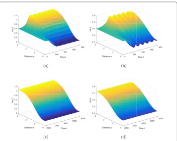
Figure 3When (μ1,μ2) = (0.22, 0.132) lies in region①, the positive constant steady stateE4(0.6115, 2.6044) is asymptotically stable, whereu(x, 0) = 0.6115 – 0.01 cosx,v(x, 0) = 2.6044 + 0.01 cosx

Figure 4When (μ1,μ2) = (0.2, 0.016) lies in region②, system (23) has two stable nonconstant steady states, whereu(x, 0) = 0.6115 – 0.001 cosx,v(x, 0) = 2.6044 – 0.001 cosxin (a) and (b) and

u(x, 0) = 0.6115 – 0.001 cosx,v(x, 0) = 2.6044 – 0.001 cosxin (c) and (d)

we know that system (23) undergoes Turing–Hopf bifurcation at P∗(A–₁,r(u4)A–₁) = (0.1388, 0.0705) (see Fig.1(a)) and

D0(α1) :α2= 0.0775α1; R1(α1) :α2=

0.0271α1– 0.007 0.02 + 0.0976α1

.

Settingn∗= 1, the normal forms truncated to the third order terms are

˙

κ= (0.0387μ1– 0.5μ2)κ– 0.0028κ3– 0.0092κϑ2,

˙

ϑ= (0.0671μ1– 0.1333μ2)ϑ– 0.0081κ2ϑ– 0.0421ϑ3.

(18)

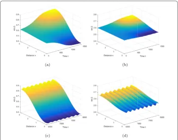
Figure 5When (μ1,μ2) = (0.4, 0.0204) lies in region③, system (23) has an unstable constant steady state E4(0.6115, 2.6044) and a stable nonconstant steady state, where

u(x, 0) = 0.6115 – 0.005 cosx,v(x, 0) = 2.6044 – 0.001 cosx. The simulate time is from 0 to 800 in (a) and (b) and the simulate time is from 2000 to 6000 in (c) and (d)

In the parameters plane (α1,α2), the dynamics of the original system (23) can be equivalent to normal forms system (39) near the Turing–Hopf bifurcation pointP∗. And we have that

κ≥0 andϑis a real number.

There exist a zero equilibriump0(for allμ1andμ2), three trivial equilibriap1,p±2, and two nontrivial equilibriap±₃ for system (39):

p0= (0, 0),

p1= (13.9353μ1– 179.8956μ2, 0), forμ2< 0.0775μ1,

p±₂ = (0,±1.5948μ1– 3.1672μ2), forμ2< 0.5035μ1,

p±₃ = (23.839μ1– 467.9284μ2,±

–2.976μ1+ 86.5523μ2)

forμ2< 0.0509μ1andμ2< 0.0344μ1.

The critical bifurcation lines are the following:

D0:μ2= 0.0775μ1; R1:μ2= 0.5035μ1;

T1:μ2= 0.0509μ1, μ2> 0; T2:μ2= 0.0344μ1, μ2> 0.

(19)

Figure 6When (μ1,μ2) = (0.1, 0.005) lies in region④, system (23) has an unstable constant steady state E4(0.6115, 2.6044) and a stable spatially inhomogeneous periodic solution, where

In region①, system (39) has an asymptotically stable equilibriump0. So system (23) has an asymptotically stable constant steady state (see Fig.3). In region②, system (39) has an unstable equilibriump0and two asymptotically stable equilibriap±2. Thus, system (23) has two stable nonconstant steady states (see Fig.4). In region③, system (39) has two un-stable equilibriap0,p1and two asymptotically stable equilibriap±₂. Hence, system (23) has two stable nonconstant steady states (see Fig.5). In region④, system (39) has four unstable equilibriap0,p1,p±₂ and two asymptotically stable equilibriap±₃. It follows that system (23) has two stable spatially inhomogeneous periodic solutions (see Fig.6). In region⑤, sys-tem (39) has three unstable equilibriap0,p±₂ and an asymptotically stable equilibriump1. Therefore, system (23) has a stable spatially homogeneous periodic solution (see Fig.7). In region⑥, system (39) has an unstable equilibriump0and an asymptotically stable equi-librium p1, which implies that system (23) has a stable spatially homogeneous periodic solution (see Fig.8).

Acknowledgements

The authors are very grateful to the referees for their valuable suggestions.

Funding

This work is supported by the Fundamental Research Funds for the Central Universities (No. 2572016CB08).

Availability of data and materials

Not applicable.

Ethics approval and consent to participate

(20)

Figure 7When (μ1,μ2) = (0.001, 0.00002) lies in region⑤, system (23) has an unstable constant steady state E4(0.6115, 2.6044) and a stable spatially homogeneous periodic solution, where

Figure 8When (μ1,μ2) = (–0.0001, –0.0002) lies in region⑥, system (23) has a stable spatially homogeneous periodic solution, whereu(x, 0) = 0.6115 – 0.3 cosx,v(x, 0) = 2.6044 – 0.2 cosx

Competing interests

The authors declare that they have no competing interests.

Consent for publication

Not applicable.

Authors’ contributions

All authors participated in the writing and coordination of the manuscript and all authors read and approved the ﬁnal manuscript.

Publisher’s Note

(21)

Received: 19 November 2018 Accepted: 29 April 2019 References

1. Yi, F., Wei, J., Shi, J.: Bifurcation and spatiotemporal patterns in a homogeneous diﬀusive predator-prey system. J. Diﬀer. Equ.246, 1944–1977 (2009)

2. Wang, J., Shi, J., Wei, J.: Dynamics and pattern formation in a diffusive predator-prey system with strong Allee effect in prey. J. Differ. Equ.251, 1276–1304 (2011)

3. Yang, R., Wei, J.: Bifurcation analysis of a diﬀusive predator-prey system with nonconstant death rate and Holling III functional response. Chaos Solitons Fractals70, 1–13 (2015)

4. Yan, X., Zhang, C.: Stability and Turing instability in a diﬀusive predator-prey system with Beddington–DeAngelis functional response. Nonlinear Anal., Real World Appl.20, 1–13 (2014)

5. Tang, X., Song, Y.: Stability, Hopf bifurcations and spatial patterns in a delayed diﬀusive predator-prey model with herd behavior. Appl. Math. Comput.254, 375–391 (2015)

6. Sun, G.: Mathematical modeling of population dynamics with Allee eﬀect. Nonlinear Dyn.85(1), 1–12 (2016) 7. Song, Y., Zhou, X.: Bifurcation analysis of a diﬀusive ratio-dependent predator-prey model. Nonlinear Dyn.78(1),

49–70 (2014)

8. Briggs, C.J., Hoopes, M.F.: Stabilizing eﬀects in spatial parasitoid-host and predator-prey models: a review. Theor. Popul. Biol.65, 299–315 (2004)

9. Wang, J., Jiang, W.: Bifurcation and chaos of a delayed predator-prey model with dormancy of predators. Nonlinear Dyn.69(4), 1541–1558 (2012)

10. Hu, D., Cao, H.: Bifurcation and chaos in a discrete-time predator-prey system of Holling and Leslie type. Commun. Nonlinear Sci. Numer. Simul.22, 702–715 (2015)

11. Zhang, H., Huang, T., Dai, L.: Nonlinear dynamic analysis and characteristics diagnosis of seasonally perturbed predator-prey systems. Commun. Nonlinear Sci. Numer. Simul.22, 407–419 (2015)

12. Huang, T., Zhang, H., Yang, H., Wang, N., Zhang, F.: Complex patterns in a space- and time-discrete predator-prey model with Beddington–DeAngelis functional response. Commun. Nonlinear Sci. Numer. Simul.43, 182–199 (2017) 13. Liang, I., Pan, H.: Qualitative analysis of a ratio-dependent Holling–Tanner model. J. Math. Anal. Appl.34, 954–964

(2007)

14. Banerjee, M., Petrovskii, S.: Self-organised spatial patterns and chaos in a ratio-dependent predator-prey system. Theor. Ecol.4, 37–53 (2011)

15. Baurmann, M., Gross, T., Feudel, U.: Instabilities in spatially extended predator-prey systems: spatio-temporal patterns in the neighborhood of Turing–Hopf bifurcations. J. Theor. Biol.245, 220–229 (2007)

16. Shi, H.B., Ruan, S.G., Su, Y., Zhang, J.: Spatiotemporal dynamics of a diﬀusive Leslie–Gower predator-prey model with ratio-dependent functional response. Int. J. Bifurc. Chaos25, 1530014 (2015)

17. Zhang, L., Liu, J., Banerjee, M.: Hopf and steady state bifurcation analysis in a ratio-dependent predator-prey model. Commun. Nonlinear Sci. Numer. Simul.44, 52–73 (2017)

18. Arditi, R., Ginzburg, L.R.: Coupling in predator-prey dynamics: ratio-dependence. J. Theor. Biol.139, 311–326 (1989) 19. Bishop, M.J., Kelaher, B.P., Smith, M., York, P.H., Booth, D.J.: Ratio-dependent response of a temperature Australian

estuarine system to sustained nitrogen loading. Oecologia149, 701–708 (2006) 20. Hanski, I.: The function response of predator: worries about scale. Trees6, 141–142 (1991) 21. Reeve, J.D.: Predation and bark beetle dynamics. Oecologia112, 48–54 (1997)

22. Nindjin, A.F., Aziz-Alaoui, M.A., Cadivel, M.: Analysis of a predator-prey model with modiﬁed Leslie–Gower and Holling-type II schemes with time delay. Nonlinear Anal., Real World Appl.7, 1104–1118 (2006)

23. Upadhyay, R.K., Rai, V.: Crisis-limited chaotic dynamics in ecological systems. Chaos Solitons Fractals12, 205–218 (2001)

24. Upadhyay, R.K., Lyengar, S.R.K.: Eﬀect of seasonality on the dynamics of 2 and 3 species prey-predator system. Nonlinear Anal., Real World Appl.6, 509–530 (2005)

25. Faria, T.: Normal forms and Hopf bifurcation for partial diﬀerential equations with delay. Trans. Am. Math. Soc.352, 2217–2238 (2000)

26. Song, Y., Zhang, T., Peng, Y.: Turing–Hopf bifurcation in the reaction-diﬀusion equations and its applications. Commun. Nonlinear Sci. Numer. Simul.33, 229–258 (2016)

27. Tang, X., Song, Y., Zhang, T.: Turing–Hopf bifurcation analysis of a predator-prey model with herd behavior and cross-diﬀusion. Nonlinear Dyn.86, 73–89 (2016)

28. Yang, R., Song, Y.: Spatial resonance and Turing–Hopf bifurcation in the Gierer–Meinhardt model. Nonlinear Anal., Real World Appl.31, 356–387 (2016)

29. Xu, X., Wei, J.: Turing–Hopf bifurcation of a class of modiﬁed Leslie–Gower model with diﬀusion. Discrete Contin. Dyn. Syst., Ser. B32(2), 765–781 (2018)