R E S E A R C H
Open Access
A comprehensive wireless sensor network
reliability metric for critical Internet of
Things applications
Dina Deif
and Yasser Gadallah
*Abstract
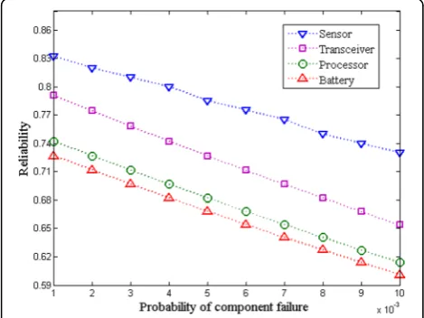
Evaluating the reliability of a wireless sensor network (WSN) deployment is a highly important task especially when the WSN is used for a critical Internet of Things (IoT) application. In this paper, we introduce a novel comprehensive reliability metric to evaluate the reliability of WSN deployments over their intended mission time. Unlike the existing studies on the topic, the proposed metric takes into account that sensor nodes (SNs) are multi-component systems that are subject to different component failures, namely, sensor, transceiver, processor, and battery failures. Consequently, SNs are modeled as three-mode (on,relay, andoff) systems instead of the simplistic two-mode (onandoff) model adopted in the existing studies. To calculate the proposed reliability metric in a computationally efficient manner, we develop a search algorithm which generates the complete path set of the given WSN deployment. Extensive experimental results demonstrate the use of the proposed metric in evaluating the reliability of several WSN deployments under different operating conditions. Results also demonstrate the computational efficiency of the developed search algorithm used for calculating the proposed metric and the significant effect of using the proposed three-mode SN model on the accuracy of the evaluated reliability.
Keywords:Wireless sensor networks, Reliability, Fault tolerance, Internet of Things, Probability of failure, Combinatorics
1 Introduction
In recent years, wireless sensor networks (WSNs) have become a versatile technology for serving a multitude of applications that include residential, industrial, com-mercial, healthcare, and military applications. As such, WSNs are considered one of the enabling technologies for realizing the Internet of Things (IoT) concept where they play the pivotal role of detecting events and meas-uring physical and environmental phenomena of interest [1]. Many of the important IoT applications served by WSNs are characterized by being mission-critical, meaning that the failure of the WSN to detect the oc-currence of an event or a phenomenon in the targeted region of interest (RoI) will have serious implications [2]. Hence, it is imperative that the WSN functions properly throughout its intended mission time. This poses stringent reliability requirements on the WSN
that must be addressed in the design and deployment phase of the network.
The first step in designing a reliable WSN is to be able to evaluate the reliability of a given WSN deployment. The reliability of any multi-component system is for-mally defined as the“probability that a system will per-form satisfactorily during its mission time when used under the stated conditions”[3]. The method by which the reliability of a specific system is evaluated varies according to the type(s) of components the system is composed of, the configuration of the system in terms of how these components are connected to each other, and the state(s) at which the system is defined to have failed. Ultimately, the reliability of the system is a func-tion of the reliability measures of its components and evaluating the reliability of the system as a whole is a probability modeling problem.
In that context, a WSN can be viewed as a multi-component system in which the multi-components are the sensor nodes (SNs) and the sink node(s). The mission time for a WSN can either be its intended lifetime or
* Correspondence:[email protected]
Electronics and Communications Department, School of Sciences and Engineering, The American University in Cairo, AUC Avenue, New Cairo 11835, Egypt
the maximum time interval between scheduled main-tenance operations. Hence, the WSN mission time is application-dependent and can vary greatly, ranging from a few days to a few years. If the WSN is composed of different types of SNs with different coverage profiles and capabilities, the WSN is said to be heterogeneous. The configuration of the WSN is determined by the way the SNs are deployed in the targeted RoI and the resulting wireless connectivity among them.
In order to identify the states at which a given WSN deployment fails, the functionality of a WSN must first be defined. The functionality of a WSN can be divided into two major elements. The first element is the sensing functionality, which is the ability of a WSN to detect all the targets or phenomena that occur inside the boundar-ies of the RoI during its mission time. Hence, for a WSN to be functional in terms of sensing, it must provide full coverage for the RoI area (in case of area coverage) or all the targeted locations in the RoI (in case of point coverage) during its mission time. The second element of the WSN functionality is the connectivity functionality, which is the ability of the WSN to deliver sensed data from its sources (i.e., SNs) to the designated destination (i.e., sink node(s)) during its mission time. Hence, for a WSN to be functional in terms of connectivity, any target or a phenomenon detected by one or more SNs has to be recognized at the sink node(s) through multi-hop wireless communication throughout the WSN mission time. Based on this definition of WSN functionality, a WSN is said to have failed if either of its sensing or connectivity functionality elements fail [4].
There are several issues that can affect the reliability of a WSN by compromising its functionality in terms of coverage and/or connectivity. These issues can generally be classified into SN-related and non-SN-related issues. SN-related issues are factors pertinent to the functional-ity of the deployed SNs, mainly, SN power failure, hard-ware failures, and softhard-ware failures. The effect of these issues on the functionality of the network during its mission time (i.e., on the reliability of the network) can be predicted [5] as will be discussed later. These issues can be summarized as follows:
SN power failure: the majority of the industrial and
commercial SNs currently available in the market are battery-powered. Current advances in the fabrication of batteries have recently introduced highly durable batteries for SNs that can last for years (e.g., lithium
thionyl chloride batteries (http://www.tadiran
batteries.de/eng/products/lithium-thionyl-chloride-batteries/overview.asp)) under certain conditions. Although these batteries can sustain the operation of the SNs for long periods of time, premature battery failures can still occur in practice. This can
be attributed to a myriad of reasons such as the deployment of the SNs in harsh environmental conditions (e.g., extreme temperatures or rain), incorrect handling or random failure caused by
defective hardware (https://www.omnisense.com/
oms_cds/media/008-002-002%20OmniSen-se%20FMS%20Sensor%20Battery%20Life.pdf).
SN hardware failures: SNs are subject to random
hardware failures. This is attributed to two main reasons. The first one is that most commercial SNs are cost-sensitive, meaning that they are not always built of the highest quality components. The second reason is that SNs are often subjected to harsh environmental conditions which can affect the
normal operation of its components [6].
SN software failures: SNs are prone to random
permanent software failures which can render them inactive, i.e., unable to sense or communicate.
On the other hand, non-SN-related issues are factors that are external to the deployed SNs such as wireless link failures (due to fading and external interference) and excessive packet collisions (i.e., internal interference in WSNs adopting contention-based medium access control). The effect of these issues on the overall net-work reliability is in general difficult to predict. The authors in [7] present a thorough study on the effects of non-SNrelated factors on the quality of wireless links in a WSN and show the complex and highly transient nature of these effects. Furthermore, the effects of the non-SN related issues on the WSN reliability are usu-ally mitigated using measures such acknowledgements and retransmissions [8].
In this paper, we derive a comprehensive WSN reli-ability metric, which considers the different SN-related
reliability issues, using a combinatorial approach. We adopt the general assumptions that the WSN is hetero-geneous and has an arbitrary deployment configuration (e.g., clustered or flat configuration). The functionality of the WSN is defined in terms of both network coverage and connectivity of the SNs to the sink node(s). We as-sume that the SNs are subject to four types of failures during the WSN mission time, namely, sensor failure, transceiver failure, processor failure, and power failure. Consequently, SNs are modeled as systems which have three modes of operation, namely,on, relay, andoff. To calculate the proposed reliability metric in a computa-tionally efficient manner, we develop a search algorithm which generates the complete paths set of the given WSN deployment.
reliability concepts which we will be using throughout this paper. The assumptions and derivation of the pro-posed reliability metric are presented in Section 4. In Section 5, we present the developed search algorithm which is used to evaluate the reliability of WSN deploy-ments based on the proposed metric. Section 6 presents the experimental results obtained from applying the pro-posed metric to case study surveillance WSN deploy-ments. Finally, the paper is concluded in Section 7.
2 Related work on wireless sensor network reliability
Several studies have addressed the issue of evaluating or estimating the reliability of WSNs. In this section, we re-view the most significant of these studies and discuss their scope and limitations. Based on this discussion, we highlight the scope and contribution of the reliability metric proposed in this paper. We classify the existing studies on WSN reliability into two major tracks. The first track focuses on evaluating the reliability of a spe-cific aspect of WSN functionality (such as packet trans-mission reliability) and/or to evaluate the reliability for one or more partsof the WSN (such as a single cluster in a cluster-based deployment). The studies which be-long to the first track may or may not assume that SNs are subject to random failures and battery energy deple-tion. On the other hand, the second track focuses on evaluating the reliability of a WSN as a whole, either as a function of time or as a probability over a given net-work mission time, assuming that SNs are subject to random failures. Studies which belong to the second track define WSN functionality in terms of coverage and/or connectivity and assume that SNs are modeled as a two-mode device (either on or off) and have a given probability of failure during the mission time of the network.
We begin by reviewing studies which belong to the first track. The studies in [9] and [10] address the prob-lem of evaluating the reliability of SN clusters in WSNs characterized by cluster-based deployments subject to random SN failures. In both studies, the authors assume that the SN clusters are non-overlapping and that each cluster has a designated cluster head which acts as a relay between the SNs in the cluster and the sink node. In [9], the authors define the reliability of a cluster as the probability of successful message delivery between the sink node and the cluster head. The authors in [10] define the reliability of the WSN as the probability that the geographical area of each cluster in the WSN is fully covered by its SNs and that the cluster head has at least one functional direct or multi-hop wireless path to the sink node. Based on this definition, they derive an ex-pression for the reliability of each individual cluster and use a Monte Carlo (MC) simulation approach to
estimate it. The main limitation of the studies in [9] and [10] is that the reliability of the WSN as a whole in terms of the reliability of its constituent clusters is not evaluated. In addition, the proposed definitions of reli-ability cannot be extended to WSNs with different de-ployment configurations such as flat dede-ployments which are non-hierarchical.
In [11], the authors propose a model for evaluating the reliability of disjoint areas in a WSN subject to two types of failure events, namely, SN failures due to battery depletion and link failures. Their proposed approach depends on dividing the targeted RoI into disjoint areas or target regions. For each region, a reliability model is constructed using a reliability block diagram (RBD) [3], which depends on the number of SNs monitoring the target region, their relative location from the sink node, and the routing protocol used in the network. There are two drawbacks of the proposed reliability modeling pro-posed in [11]. The first drawback is that the model does not provide a method by which the reliability of the en-tire WSN deployment can be evaluated in terms of the reliability of its regions. The second drawback is that the reliability modeling is carried out under the assumption that the probabilities of link failures are known and are constant throughout the lifetime of the WSN. This as-sumption is unrealistic since link quality is affected by numerous factors such as multi-path effects, shadowing (due to static and mobile obstacles), and interference. The effect of these factors on link quality varies signifi-cantly and rapidly in time and space [7] and hence, un-like SN-related factors, cannot be reduced to a constant probability of failure throughout WSN mission time. In [12], the authors consider the problem of evaluating the transmission reliability of cluster-based and mesh-based WSN deployments. They define transmission reliability as the ratio of the packets received by a destination node to the whole packets generated by the transmission for a given period of time. They present transmission reliabil-ity evaluation models for the uplink and downlink traffic based on the assumptions that SNs are not subject to any hardware failures and that SNs only fail when their initial battery energy is exhausted. Although the time-dependent models presented in [12] can help assess the transmission reliability over time for a given routing strategy, they are limited by the assumption that SNs cannot fail due to random hardware failures unrelated to battery exhaustion. Also, it is not possible to use the study in [12] to calculate or estimate the reliability of the WSN over a given mission time since coverage functionality is not considered.
intrusion, based on the aggregated data from several SNs in the network, as a weighted voting system (WVS). They assume that both the SNs and the wireless links between the SNs and the sink node have known misde-tection probabilities. Based on these assumptions, they derive the reliability of the sink’s WVS using the univer-sal generating function (UGF) method. Similar to the study in [12], the scope of the study in [13] does not in-clude evaluating the reliability of the WSN as a whole over a given mission time, since it is restricted to evaluat-ing the reliability of detectevaluat-ing a sevaluat-ingle target/phenomena based on a fraction of the SNs in the WSN.
On the other hand, the studies in [14, 15] belong to the second track since they address the reliability of SN systems or WSNs as a whole of non-hierarchical deploy-ment configurations subject to random SN failures. In [14], the authors address the problem of evaluating the reliability of WSNs designed for industrial inventory management. They assume that for the purposes of this specific application, the data collected by each SN are stored redundantly on several other SNs to account for random SN failures. Accordingly, the WSN is deemed functional as long as there is a sufficient number of functional SNs that are both connected to each other and to the sink node. Based on this definition of network functionality and the assumption that the WSN deploy-ment is homogeneous, the reliability evaluation problem is reduced to the famous K-out-of-N reliability problem (http://www.reliabilityanalytics.com/blog/2011/09/02/ reliability-modeling-k-out-of-n-configutation/). The au-thors also present a Monte Carlo (MC) simulation ap-proach similar to that proposed in [10] to estimate the reliability of the WSN at hand. However, the reliability evaluation and estimation approaches proposed in [14] are based on a very restrictive definition of network functionality. Consequently, they cannot be applied to other WSN applications (e.g., surveillance and monitor-ing applications) where the functionality of the network is dependent not only on the number of SNs connected to the sink node but also on the network coverage. Also, the proposed approaches do not support network het-erogeneity which is a major limitation since real-world deployments are often heterogeneous.
The authors in [16] propose a reliability metric for SN systems designed for surveillance purposes subject to random SN failures. They assume an arbitrary deploy-ment configuration where SNs can monitor multiple tar-get locations in the RoI and that each tartar-get location can be monitored by multiple SNs. They also assume that the surveillance SN system can be heterogeneous. The reliability of the system is defined as the probability that all target locations are monitored by at least one SN. The authors use a combinatorial approach to formulate the proposed reliability metric and present a search
algorithm to calculate the proposed reliability metric in a time-efficient manner. The main limitation of the pro-posed metric is that system functionality is assumed to be in terms of the degree of target locations coverage only. Connectivity between SNs to form a wireless net-work is not considered.
The study in [17] propose a method for evaluating the reliability of WSNs designed for industrial IoT applica-tions based on the automatic generation of fault trees (FTs). The proposed method requires the network failure conditions as inputs to enable the generation of the corresponding network FT and compute the network reliability. A network failure condition is defined as a combination of SNs which if fail will lead to the failure of the WSN in terms of network coverage only and not connectivity to the sink. To address the connectivity part of the network functionality, the authors propose a depth-first search algorithm that finds all the paths be-tween SNs belonging to the network failure conditions and the sink node. The study in [17] is extended in [15] by assuming that the WSN is also subject to permanent wireless link failures in addition to SN failures under the same assumptions adopted in [17]. In both studies, the authors in [17] and [15] did not address the computa-tional efficiency of their approach.
In this study, we focus on the second track, i.e., on the problem of evaluating the reliability of the WSN a whole, defined as the probability that the WSN is func-tional during a given mission time, assuming that SNs are subject to random permanent failures. Based on the above discussion, existing studies in that track all as-sume that SNs have only two modes of operation, either
onoroff. If an SN ison, it is assumed to be functional in terms of both sensing its surrounding environment and communicating wirelessly with its neighbors. If it is off, then the SN has failed permanently due to one or more of the SN-related reliability issues outlined in Section 1. This representation is not accurate since most commercial SNs are composed of multiple independent chips that carry out different functions, with each having its own probability of failure during the network’s mission time.
A more accurate model considers the SN as a multi-component system [18]. Based on this model, an SN has three modes of operation. These modes of operation are
is adequately defined in terms of both network coverage and connectivity. The addition of therelay mode to the SN model provides a more accurate evaluation of WSN reliability because it avoids the under-evaluationof the WSN reliability when the conventional two-mode SN model is used. Under-evaluation of the reliability of the network becomes an issue when the reliability is used as a requirement/constraint for WSN deployment. In that case, the network designer aims to deploy sufficient SNs to achieve a minimum level of network reliability while minimizing the number of deployed SNs, i.e., minimizing the deployment cost. In that case, under-evaluating the re-liability of a given deployment can lead to an unnecessary increase in the deployment cost. The second advantage is that it enables the network designer to isolate the effect of the quality (i.e., reliability) of the individual components of the deployed SNs (i.e., sensor, transceiver, processor and power unit) on the overall reliability of the WSN. This is discussed in more details in Section 4.1.
In this paper, we derive a comprehensive WSN reli-ability metric which takes into account the different SN-related reliability issues using a combinatorial approach. Compared to the existing reliability evaluation and esti-mation approaches, the strengths of our proposed metric can be summarized in the following points:
Network functionality is defined in terms of both
network coverage of a predefined set of target locations in the RoI and connectivity to the designated sink node.
No specific network deployment configuration is
assumed in the proposed model. We assume an arbitrary deployment configuration where each deployed SN may monitor multiple target locations in the RoI and each target location may be monitored by multiple SNs. All SNs can communicate wirelessly with their neighbors, i.e., no imposed communication hierarchy.
The WSN can be heterogeneous; it can consist of
more than one type of SNs, each characterized by a different coverage profile and set of capabilities.
A more realistic SN model is adopted in the
derivation of the proposed metric where an SN has three modes of operation instead of the two-mode model used in the existing studies.
Each SN type is characterized by four different
probabilities of failure during the mission time of the network (namely, sensor, transceiver, processor, and battery probabilities of failure) instead of a single SN probability of failure, as it is the case in the existing studies.
A search algorithm is developed to calculate the
propose reliability metric in a computationally efficient manner.
In this study, we assume that wireless links between SNs are not subject failure. This assumption is justified as follows. Wireless link quality is affected by numerous factors such as multi-path effects, shadowing (due to static and mobile obstacles), and interference. The effect of these factors on link quality varies significantly and rapidly in time and space [7] and hence, unlike SN-related factors, cannot be reduced to a constant prob-ability of failure throughout WSN mission time. On the other hand, permanent wireless link failures are mainly due to a complete failure (i.e., a failure in the transceiver, processor, or battery) in one or both SNs at the ends of the link [19]. In the proposed metric in this paper, this type of failure is taken into consideration since we as-sume that each of the main SN components are subject to failure with a given probability of failure during the WSN mission time.
3 Fundamental reliability concepts
In this section, we discuss some of the fundamental defi-nitions and concepts related to the evaluation of multi-component systems’ reliability which we will be using throughout this paper.
3.1 Component reliability function and component reliability
The main objective of reliability modeling is to express the reliability of a given system in terms of the reliability measures of its constituent components. There are two main reliability measures for any device or component. The first measure is the reliability function Rc(t), which is used to estimate the probability that the device or component will continue to function beyond a time dur-ation of length t [3]. The second reliability measure is based on the fact that for most practical purposes, a device or component is only required to function during the spe-cified mission timeTmof the system it belongs to. In this case, the reliability functionRc(t) can be substituted by the reliability of the device. The reliability of a device, Rc, is simply defined as the probability that the device will con-tinue to function throughout the mission time of the sys-tem. Accordingly, the probability of failure of the device duringTmis equal to 1−Rc(Tm) = 1−Rc[3].
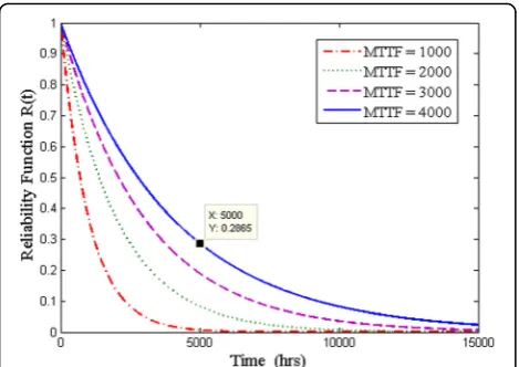
For example, Fig. 1 shows an exponential reliability function, which is one of the simplest functions used in modeling the reliability of electronic components. The exponential reliability function which is Rceð Þt is given by the following equation:
Rceð Þ ¼t e
−αt; ð1Þ
equal to the reciprocal of its mean time to fail (MTTF). From the reliability curves in Fig. 1, we can estimate the reliability at t= 5000 h for α= 1/4000 (i.e., for MTTF = 4000) to be 0.287. This in turn means that there is a 1−0.287 = 0.713 chance that the component will fail during this time interval, i.e., the probability of failure during this time interval is 0.713.
Although the exponential reliability function is com-monly used in reliability engineering due to its simpli-city, it usually leads to inaccurate estimations of the probabilities of failures. This is because this type of func-tion is based on the assumpfunc-tion that the component has a constant failure rate, which means that its performance does not degrade with time. To obtain a more accurate model for the reliability function of a given electronic device, reliability engineers carry out rigorous reliability testing techniques and/or gather empirical data on the device in service [3]. For example, qualitative and quan-titative accelerated reliability testing is used to identify probable hardware failures of SNs and estimate the probability of their occurrence [5].
3.2 Combinatorial approach to system reliability evaluation
Combinatorics is a proven useful tool in evaluating and estimating the reliability of complex systems and net-works [20, 21]. The fundamental premise of the com-binatorial approach to reliability evaluation is that the reliability of any system can be computed by means of evaluating the system’s structure function for every possible state of the system. To explain this concept, consider a system S which consists of n components, i.e.,S= {1, 2,….,n}. Each component can only have two distinct states: it can either be functional or on or it can fail or beoff. Let the binary variableπibe the state indicator of componentias follows:
πi¼ 1; if component i is on
0; if component i is off
ð2Þ
A stateπof the systemSis a description of the states of all its components, hence π= {πi} for i= 1 ,…,n. LetΠ be the set of all possible states ofS. The structure function of S, denotedf(π), is a binary function that in-dicates whether the system is working under a given state according to the following equation:
fð Þ ¼π 1; Sis functional
0; Shas failed
ð3Þ
Based on the above definitions, the reliability of S, denoted by R(S), can be calculated using the following equation:
Rð Þ ¼S Probðfð Þ ¼π 1Þ ¼X
π∈Π
fð Þπ :Probð Þπ ð4Þ
To calculate R(S) using (4), the conditions necessary for Sto be functional must be defined and the probabil-ity of any system state must be evaluated in terms of the reliabilities (or probabilities of failure) of the system’s components, assuming that the system has a specified mission time Tm. Theoretically, f(π) must be evaluated for all the possible system statesπ∈Π to calculate R(S) using this approach. However, following this extensive method in reliability calculation poses a computational problem for systems of a practical scale. For example, a system composed of 30 components which fail inde-pendently has 230 states. Therefore, a tremendous amount of time is required to calculate R(S) which grows exponentially with the number of components in the system. This computational problem is mitigated by the use of more efficient methods (e.g., reliability block diagram (RBD), fault tree (FT), and search algo-rithms) that attempt to find all the system’s path sets or cut sets [20].
To define a system’s path and cut, letS1(π) be the set of functioning components, i.e., components in the on
state, in S for a given system stateπ and S0(π) be the set of failed components, i.e., components in the off
state.S1(π) andS0(π) can be expressed by the following equations:
S1ð Þπ ≡fijπi¼1; i∈Sg; ð5Þ
S0ð Þπ ≡fij πi¼0; i∈Sg; ð6Þ
where S1(π)∪S0(π) = S. A state π of the system S is called a path if f(π) = 1. In that case, the corresponding path set is the setS1(π), i.e., a path set is the set of com-ponents whose simultaneous functional state guarantees that the overall system is functional. On the other hand, a state π of the system S is called a cut if f(π) = 0. In this case, the corresponding cut set is the set S0(π). That Fig. 1Exponential reliability function plot for different values of
is, a cut set is the set of components whose simultan-eous failure results in the failure of the overall system. If all the path sets or alternatively all the cut sets of a sys-temSare known, we can rewrite (4) as follows:
Rð Þ ¼S Xπ∈Π
1Probð Þ ¼π 1−
X
π∈Π0Probð Þπ ; ð7Þ
where Π1 is the set of all the paths of S (i.e., the complete paths set of S ) and Π0 is the corresponding set containing all the cuts of S (i.e., the complete cuts set ofS) such that Π1∪Π0=Π . For example, a simple system of n components connected in series has only one path set which is equal to the system set S= {1, 2, ….,n} and has Pnk¼1Cn
k cut sets. Therefore, it is simpler
to express its reliability as R(Sseries) = Prob(π= {πi= 1, ∀i= 1 ,…,n}) ¼Qin¼1Ri, where Ri is the reliability of the ith component during the system’s mission time. On the other hand, a system of n components con-nected in parallel has only one cut set which is equal to S and has Pnk¼1Cnk path sets. Hence, the system’s reliability can be expressed as RSparallel¼1−Prob
π¼fπi¼0;∀i¼1;…;ng
ð Þ ¼1−Qn
i¼1ð1−RiÞ.
4 Reliability of wireless sensor networks
In this section, we use the combinatorial approach out-lined in Section 3 to derive the reliability of a WSN with an arbitrary deployment configuration. We start by mod-eling the SN as a multi-component system and identify-ing its different states and modes of operation. Then, we present the WSN model and define the conditions re-quired for the WSN to be deemed in working condition. Finally, we derive the reliability of the WSN in terms of its structure function and the probabilities of failure of its constituent SNs’hardware components.
4.1 Sensor node model
Although SNs vary greatly in terms of their capabilities (e.g., processing power, battery capacity), there are four fundamental chips or components that are common in all SNs [22]: a sensing unit(s) or simply sensor(s), a radio unit or transceiver, a processing and memory unit or processor, and a power unit or battery. The sensor is responsible for the translation of physical phenomena detected/measured in the RoI to electrical signals. The transceiver enables the SN to communi-cate wirelessly with its neighboring SNs and with the sink node. The processor is responsible for perform-ing all required computations and controllperform-ing both the sensor and transceiver. The battery supplies all three components with power. The type and capacity of the SN battery is carefully chosen according to the application and the required mission time of the WSN
(http://www.sensorsmag.com/components/a-practical- guide-to-battery-technologies-for-wireless-sensor-networking).
Each of these components is subject to random failure [6], [23] due to several reasons such as faulty hardware, faulty software, harsh environmental conditions, and degradation with time. Accordingly, each of the SN’s four main components has a given reliability or, alterna-tively, a probability of failure during the WSN mission timeTmas defined in Section 3.1. As mentioned earlier in Section 3, the reliabilities of the different components of an SN can be estimated through a standard reliability prediction test provided by the SN vendor or through reliability testing techniques [5].
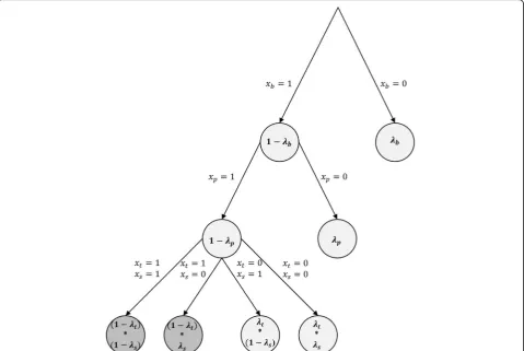
Since each of the four components can either function or fail, i.e., be in an onoroffstate, an SN can theoretic-ally have 24 possible states. To describe these states, let the binary variables xs, xt, xp, and xbbe the state indi-cators of the sensor, transceiver, processor, and battery, respectively, of an SN as defined in (2). Hence, an SN state x is described using a tuple of these four vari-ables {xs, xt,xp, xb}. These variables are not statistically independent; the sensor and transceiver cannot possibly function if either the processor or the battery fails. There-fore, some of the SN states are practically impossible, and hence, their probability of occurrence is zero.
To calculate the probability of occurrence of the other possible states, let λs, λt,λp, and λb be the probabilities of failure of the sensor, transceiver, processor, and bat-tery, respectively. It should be noted that the estimated probability of failure for any given device or hardware component is obtained regardless of the failure of any other device or component. Hence,λsandλtare actually the probability of failure of the sensor and transceiver conditioned on the event that the component is properly controlled (i.e., processor is functional) and powered (i.e., battery is functional). Similarly,λpis the probability of failure of the processor conditioned on the event that the battery is functional, where as λb is the uncondi-tional probability that the SN power unit or battery fails during Tm. According to the above definitions, the probability of an SN state can be given by the following equations:
probability. It is straightforward to verify that the sum of the probabilities of these states is equal to unity. There are two SN states at which the SN is of use to the WSN. The first state is described by the tuple {1,1 , 1,1}, at which all four components are functional and the SN can both sense its surroundings and communicate wire-lessly. This state corresponds to the on mode of oper-ation in which the SN is fully functional as defined in Section 1. The second state is described by the tuple {0,1 , 1,1} at which only the sensor(s) failed and the SN can only communicate wirelessly, i.e., acts as a relay node. This state corresponds to therelay mode of operation in which the SN is partially functional as de-fined in Section 1. In all the practically possible remaining states, the SN does not serve the network, and hence, a SN in these states is considered to be in theoffmode of operation.
4.2 Wireless sensor network model
We assume that the targeted RoI of the WSN is a two-dimensional area in which there is a finite set of locations
that require some form of monitoring (e.g., motion, image, video) using static SNs. These locations are called
sensory data acquired by the SNs should be relayed to a sink node with an arbitrary fixed position in the RoI through wireless multi-hop communications. We assume that all deployed SNs have a fixed communication range,
rc. Hence, any two SNs deployed have a wireless commu-nication link if the distance between them is less than or equal torc. Naturally, it is required that the WSN remains functional in terms of coverage and connectivity through-out its intended mission timeTm. To express this math-ematically, we use the following definition:
Definition:A WSN is said to be functional in terms of both coverage and connectivity if both of the following two conditions are met:
1. Each target pointtjforj= 1 ,…,mis covered by at
least one SN with an uncompromised sensing
capability, i.e., an SN in theonstate. Let the setYj
be the set of SNs in theonstate that monitortj.
Then this condition can be expressed as, |Yj|≠0 ,
∀j= 1 ,…. ,m where |.| denotes the size of a set.
2. Within each Yj,there is at least one SN that has at
least one functional path to the sink node. This implies that SNs along that path, including the source SN, have uncompromised communication
capabilities, i.e., in either theonor therelaystate.
Hence, the events detected at anytjcan be relayed
back to the sink node. Let the set Zjbe the set of
SNs which belong toYjthat are connected to the
sink node. Hence, Zj⊆Yj. The condition can be
expressed as |Zj|≠0 , ∀j= 1 ,…. ,m.
In the next subsection, we will use the above definition of WSN functionality conditions in defining the structure function of the WSN, which we defined in Section 3.2.
4.3 Wireless sensor network reliability metric derivation
The reliability of the WSN, S, denoted by R(S), is de-fined as the probability that the WSN remains func-tional, in terms of coverage and connectivity, subject to four types of SN component failures during its intended mission time, Tm. In order to use the combinatorial ap-proach outlined in Section 3.2 to derive R(S), we must define the states of S and its structure function. To de-fine the states of S, letXs,Xt,Xp, and Xbbe the subsets of SNs inSthat have failed sensors, transceivers, proces-sors, and batteries, respectively. Hence, a state of the WSN S is described by the tuple π≡{Xs,Xt,Xp,Xb}, whereXs,Xt,Xp,Xb S. Therefore, each state πis as-sociated with a unique combination of SN components’ failures. To calculate the probability of occurrence of a given state, π, the corresponding statexi(π) of each indi-vidual SN si∈Smust be identified. Assuming the com-ponents belonging to different SNs fail independently,
Prob(π) can be expressed by:
Probð Þ ¼π ProbXs;Xt;Xp;Xb
¼YNi¼1Prob xð ið Þπ Þ ð9Þ
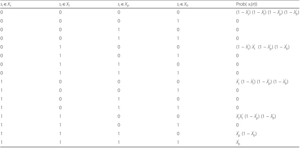
Table 1 lists the different values of the probability of an individual SN state xi(π) for a given network state π based on the SN states illustrated in Fig. 2. The first state in Table 1 corresponds to a SN in the on
mode, the ninth state corresponds to the relay mode, while the rest of the non-zero probability states corres-pond to theoffmode as illustrated in Fig. 2.
its functionality conditions in terms of both coverage and connectivity under a specific combination of SNs components failures. Let Π be the set of all possible states of S. Based on the definition provided in the previous subsection, the structure function of Scan be expressed as follows:
fð Þ ¼π 1; if Zj⊆Yj≠ϕ ∀j¼1;…;m
0; otherwise
ð10Þ
Similar to (3), we can now express the reliability of the WSNSas follows:
Rð Þ ¼S ProbðSis functional duringTmÞ ¼ X
πΠ
fð Þπ:Probð Þπ
½
¼ X
Xs⊆S
X
Xt⊆S
X
Xp⊆S X
Xb⊆S
fXs;Xt;Xp;Xb: YN
i¼1Probðxið ÞπÞ
h i
ð11Þ
Equation (11) states that the reliability of the WSN is the summation of all the probabilities of the WSN states that have a structure function value of unity (i.e., the probabilities of all the paths of the WSN S). Depending on the set of failed components in the stateπ, the indi-vidual probabilities Prob(xi(π)) ,i= 1 ,…N can be calcu-lated using Table 1.
5 Reliability metric calculation
From the derived expression of R(S) in (11), it is clear that the reliability calculation involves in turn evaluating
the structure function of the network, f(π), for all possible states of S, i.e. for all πϵΠ. As explained in Section 3.2, this can pose a computational challenge since WSNs designed for practical purposes are often composed of tens of SNs, resulting in a huge number of possible network states. This problem is further complicated by modeling the SNs as four-component systems which in turn have multiple possible states. For example, a WSN composed of just 30 SNs would have 24∗30= 2120 states. This means that the calcula-tion of the reliability metric in this case would require a prohibitive amount of time. To solve this computa-tional problem, we make use of the following two properties of the WSN, S, using the model presented in Section 4.2:
The majority of the network states have null
probabilities, and hence, they do not contribute
to the value of R(S). This stems from the fact the
majority of the individual SN states also have a null probability (i.e., are not practically possible)
as shown in Table1.
The WSNShas the property of being a monotone/
coherent system [21]. This property implies the
following. If the failure of a set of SNs’components
causesSto fail, then the failure of any set which
contains this set will also causeSto fail. For
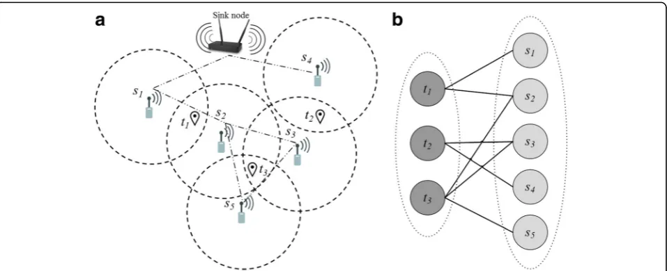
example, if we assume that the SNss1ands2in the
WSN depicted in Fig.3a are both in theoffmode
while the remaining SNs are in theonmode, then it
Table 1Evaluation of the probability of the corresponding individual SN states for a given WSN state=Xs,Xt,Xp,Xb},where“true” and“false”are denoted by 1 and 0, respectively, andλis;λit;λip,λibare the probabilities of failure of the four main components of SNsi
si∈Xs si∈Xt si∈Xp si∈Xb Prob(xi(π))
0 0 0 0 (1−λis) (1−λit) (1−λip) (1−λib)
0 0 0 1 0
0 0 1 0 0
0 0 1 1 0
0 1 0 0 (1−λis)λti (1−λip) (1−λib)
0 1 0 1 0
0 1 1 0 0
0 1 1 1 0
1 0 0 0 λis(1−λti) (1−λip) (1−λib)
1 0 0 1 0
1 0 1 0 0
1 0 1 1 0
1 1 0 0 λisλit(1−λip) (1−λib)
1 1 0 1 0
1 1 1 0 λip(1−λib)
can be readily observed that this would causeSto
fail since any phenomenon at target pointt1cannot
be detected or communicated to the sink node. This means that network states corresponding to this situation have a structure function value of zero as expressed in (10). Using the monotone property, we can say that the network states that
include the SNss1ands2being in theoffmode
ands4being in therelaymode would also have a
structure function value of zero without actually evaluating the function.
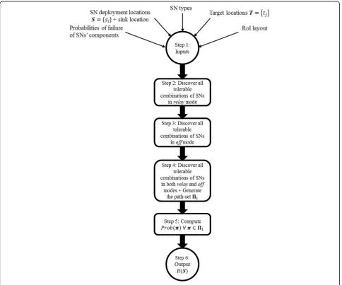
These two useful properties are used to develop a Breadth-First Search (BFS) algorithm that generates the complete path set of S, denoted by Π1, and use it to calculate R(S) using (11). The general structure of the developed search algorithm is illustrated in Fig. 4. The pseudo-code of the algorithm, which provides execution
details, is given in Table 2. The structure of the algorithm can be summarized in the following steps. In step 1, all the required parameters for the calculation of
R(S) are specified as inputs. This includes the two-dimensional RoI layout, the positions of the target locations within the RoI provided by the set of target points T= {tj}, the positions of the deployed SNs pro-vided by S= {si},the types of the deployed SNs includ-ing their coverage profiles and wireless communication ranges, and the probabilities of failure of the SN com-ponents associated with each SN type. We assume here that the sink node can be at any fixed arbitrary position in the targeted RoI. We initialize the value ofR(S) with the probability of the network state π which corre-sponds to all the deployed SNs being in the on mode. Since this network state is an obvious path of S , we also initialize the network path setΠ1with this state as expressed in 1.c. in Table 2.
Whether any other given state π is a path of the net-work or not (i.e., whether f(π) = 1 or 0) depends on the WSN configuration/topology. To evaluate f(π), the two conditions of WSN functionality, namely, coverage and connectivity, are checked according to the same defini-tions and order presented in Section 4.2. Checking the WSN coverage is straightforward and has the computa-tional complexity ofO(n∗m). If one or more of the target points in the RoI is uncovered, then f(π) = 0 and the
connectivity condition does not need to be checked. Checking the WSN connectivity condition is more complex computationally, and it depends on the con-nectivity matrix between the SNs and the sink. Con-structing that matrix has the complexity O(n2). For every WSN state π, the connectivity matrix is updated according to SNs’modes in the stateπand the updated connectivity matrix is used to check the connectivity condition. We carry out this check using the
Floyd-Table 2Pseudo-code for the proposed algorithm for calculating the reliability of a WSNS
Step Algorithm for computing WSN reliabilityR(S)
1.a. Set all parameters (S= {si},T= {tj}, types of SNs, sink location,λis,λit,λipandλibfori= 1 ,…,nandj= 1 ,…,m)
1.b. InitializeR=Prob(π|si∈Sis inonmode∀i= 1 ,…,n)
1.c. InitializeΠ1= {(π|si∈Sis inonmode∀i= 1 ,…,n)}
2.a. Letkbe the number of SNs inrelaymode. Initialize k= 1.
2.b. Letℱkr be ak−combination of SNs inrelaymode. LetFkr be the set ofk−combinations of SNs inrelaymode thatScan tolerate. Initialize ℱk
r ¼Fkr¼f gϕ .
2.c. Fori= 1 ,…,n
- Letsibe inrelaymode, i.e.ℱkr¼f gsi
- Evaluatef πjℱk r
using (10) - Iff πjℱkr
¼1→Fkr ¼Fkr∪ℱkr
End For loop
2.d. While Fkr≠f gϕ → k¼kþ1, LetFrlk−1∈Frk−1; ℱk
r¼Fkr ¼f gϕ
2.e. Forl¼1;…;jFrk−1jandi= 1 ,…,n
- Letℱk
r ¼ Frlk−1;si
- Evaluate f πjℱkr
using (10)
- Iff πjℱkr
¼1→Fkr ¼Fkr∪ℱkr
2.f. End For loops, End While loop
3.a. Letkbe the number of SNs inoffmode. Initialize k= 1.
3.b. Letℱkobe ak−combination of SNs inoffmode. LetFkobe the set ofk−combinations of SNs inoffmode thatScan tolerate. Initialize ℱk
o¼Fko¼f gϕ .
3.c. Repeat step 2.c. foroffmode, i.e.ℱk
o¼f gsi
3.d. While Fk
o≠f gϕ → k¼kþ1, LetFolk−1∈Fok−1; ℱk
o¼Fko¼f gϕ
3.e. Repeat 2.e. usingFolk−1andℱkoto get Fko
3.f. End For loops, End While loop
4.a. Letℱrandℱobe a combination of SNs inrelayandoffmodes respectively.
LetFrandFobe the sets of all combinations of SNs of inrelayandoffmode that thatScan tolerate respectively.
LetFrlr∈FrandFolo∈Fo
4.b. Forlr= 1 ,…, |Fr| and lo= 1 ,…, |Fo|
- Let ℱr¼Frlrandℱo¼Folo
- Evaluatef(π|ℱr,ℱo) using (10)
- If f(π|ℱr,ℱo) = 1→Π1=Π1∪π
End For loops
5.a. Letπl∈Π1
5.b. Forl= 1 ,…, |Π1|
-R(S) =R(S)+Prob(πl)
End For loop
Warshall algorithm (https://en.wikipedia.org/wiki/Floyd% E2%80%93Warshall_algorithm), which can compute the shortest paths (if one exists) between all SNs (in theonor
relay mode) and the sink node with the computational
complexityO(n3). If all the SNs covering any given target point do not have a path to the sink node,f(π) = 0, other-wise connectivity is intact andf(π) = 1.
In step 2, the algorithm searches for all the combina-tions of SNs that can be in the relay mode without compromising the functionality of S, assuming the re-mainder of the deployed SNs are in theonmode. These SN combinations are referred to as the“tolerable com-binations of SNs in the relay mode.” This means that for the network states corresponding to these SN com-binations, the structure function f(π) expressed in (10) is equal to unity. To perform the required search in step 2, we define Fk
r as the set that holds the tolerable
combinations of SNs inrelaymode of lengthk starting with k= 1 as expressed in 2.a–2.c. in Table 2. For ex-ample, consider the WSN depicted in Fig. 3a. The set of single tolerable SNs in the relaymode will be given by F1
r ¼ff gs1 ;f gs2 ;f gs3 ;f gs4 ;f gs5 g. The algorithm
then proceeds with the search for an increasing value of
k as expressed in 2.d–2.f. in Table 2. For example, the combination {s1,s3} belongs to F2
r while {s1,s2} does
not. This search continues until the algorithm reaches a value ofkwhich results in an empty Fkr, i.e., Fkr ¼f g∅ . The set of all tolerable combinations of different lengths of SNs inrelaymode is denoted Fr.
In step 3, the algorithm searches for all the combi-nations of SNs that can be in the off mode without compromising the functionality of S , assuming the remainder of the SNs is in the on mode, i.e. tolerable combinations of SNs in the off mode. The search fol-lows the same procedure in step 2. We define Fk
o as
the set that holds the tolerable combinations of SNs in the off mode of length k. Using the same example WSN in Fig. 3a, F1o¼ff gs2 ;f gs3 ;f gs4 ;f gs5 g. The
combination {s4,s5} belongs to F2
o while {s2,s5} does
not. The set of all tolerable combinations of different lengths of SNs in the offmode is denoted Fo.
In step 4, the algorithm uses the setsFr andFo to dis-cover all the pairs of combinations of SNs that can be in
the relay and off modes simultaneously without
com-promising the functionality of S, assuming the remain-der of the SNs is in the on mode. For example, the combination {s1,s3} can be in the relay mode while {s5} can be in the off mode simultaneously without causing the WSN depicted in Fig. 3a to fail. Each of the discov-ered pairs of combinations corresponds to one or more distinct network path and hence the complete path set
Π1is updated accordingly as expressed in 4.b in Table 2. In step 5, the probabilities of the network paths in Π1
are calculated using (11) and Table 1. Finally, the reli-ability of the given WSNR(S) is calculated using (7) and given as an output in step 6.
6 Case study
6.1 Experimental setup
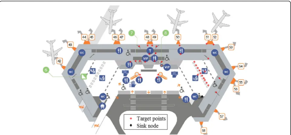
In this section, we apply the reliability metric that we proposed in Section 4 and the search algorithm pro-posed in Section 5 to evaluate the reliability of a surveil-lance WSN designed to cover part of an international airport terminal. Figure 5 shows the layout of the airport terminal (http://www.aeroflot.ru/cms/en/before_and_after_ fly/terminal_info.), which comprises the RoI of the WSN. Target points, marked on the figure in red, represent the vital locations that need to be placed under image/video surveillance such as arrival checkpoints, entrances, and staircases. The sink node to which all SNs in the WSN should be connected is marked in black.
To obtain our test deployments of the WSN, we use the Variable Length Genetic Algorithm (VLGA) pre-sented in [24]. This optimization algorithm is designed to obtain cost-optimized deployments for heteroge-neous WSNs that fulfill specific design objectives using a variable-length chromosome integer-encoded GA. In [24], the only considered design objective is providing coverage for all the target points in the RoI, i.e., provid-ing full-coverage of the set T= {tj} for j= 1 ,…,m. However, since a well-designed surveillance WSN should be functional in terms of coverage and connectiv-ity, as defined in Section 3.2, we modified the VLGA in [24] to add network connectivity to the design objec-tives. To achieve this, we modify the fitness function that is used to evaluate the fitness of the candidate deployments or chromosomes in [24], as follows:
f c lð ð ÞÞ ¼− X
which runs on an Intel processor Core i7-3621QM CPU, 2.1 GHz and 6 GB of RAM.
To demonstrate the proposed metric ability to evaluate the reliability of heterogeneous deployments, we assume that there are two types of SNs available for the deploy-ment of the WSN. The coverage profile parameters and probabilities of failure of the SNs’components for each SN type are listed in Table 3. We assume that both SN types have a coverage range and a communication range of 30 and 40 m, respectively. Although the exact reliabil-ity figures for commercial SNs such as Tmote2 and Iris nodes are not publicly available, we estimated the given probabilities of failure using the reliability figures avail-able for Texas Instrument CC2420 IEEE 802.15.4 trans-ceiver (http://www.ti.com/product/CC2420/quality) as a reference point, assuming a WSN mission time of 5 years. We also used the fact that sensor hardware is the SN component most prone to failure [6] and that the premature battery failure rate for the highly durable lithium thionyl chloride batteries recently used for SNs is very low (https://www.omnisense.com/oms_cds/media/ 008–002-002%20OmniSense%20FMS%20Sensor%20 Battery%20Life.pdf ).
To thoroughly evaluate the proposed metric in terms of the computational efficiency, it is crucial to assess the effect of the deployment size and complete path set
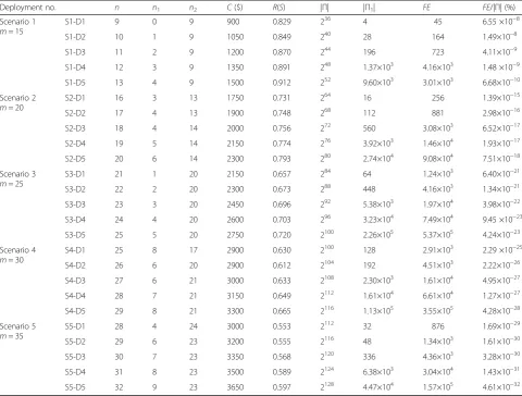
size |Π1| for a given deployment on the computation time of the proposed algorithm outlined in Table 2. To achieve this objective, we apply the VLGA to obtain cost-optimized deployments for five target point sets of sizes m= 15 , 20 , 25 , 30, and 35. For each deployment scenario, i.e., for each value of m, we obtain five de-ployments of different sizes (i.e., different values ofn), with the deployment of the smallest size being the most cost-optimal and the deployment with the lar-gest size being the least cost-optimal. Each deploy-ment fulfills the coverage and connectivity network functionality conditions in the case of no SN failures and has a different level of SN redundancy, where the higher the n, the higher the redundancy level and the larger the complete path set Π1and vice versa. Data of the resulting 25 deployments, including the size of the deployment (n), number of SNs of each type (n1 and n2), and the total deployment cost (C), are pre-sented in Table 4.
6.2 Results and discussion
To evaluate the computational efficiency of the proposed al-gorithm outlined in Table 2, we use the alal-gorithm to evalu-ate the reliability of the WSN deployments in Table 4. For each deployment, Table 4 shows the value of the reliability
R(S) , the total number of possible network states |Π| (which
Table 3Parameters of the SN types used in the deployment of the case-study surveillance WSN
FoV rs rc λs λt λp λb Price($)
Type 1 90° 30 m 40 m 1.0 ×10⁻² 5.0×10⁻³ 2.0×10⁻³ 1.0×10⁻³ 150
Type 2 60° 30 m 40 m 1.5×10⁻² 5.5 ×10⁻³ 2.5×10⁻³ 1.5×10⁻³ 100
is equal to 24∗n), the size of the deployment complete path set |Π1| , the number of network structure function evalua-tions FEperformed by the algorithm, and the value of the ratioFE/|Π1| in percentage points. The latter ratio is used as a measure of the computational efficiency of the pro-posed algorithm. This is because the most computationally expensive sub-routine in the algorithm is the evaluation of the network structure function expressed in (10). For each structure function evaluation, checking the two network functionality conditions, i.e., checking the network coverage of the set of target points and the connectivity to the sink, has a computational complexity of O(n∗m) and O(n3), re-spectively. Therefore, the computation time of the algo-rithm is mainly determined by the number of structure function evaluations denoted byFE.
It can be readily observed that the values of R(S), |Π1|, andFE increase steadily with the increase of n in each deployment scenario. This behavior is expected and is attributed to the increase in the level of SN redun-dancy in the deployment as n increases. An increase in the level of SN redundancy translates to an exponential
increase in the number of the paths of the deployment and hence the increase of the reliability R(S). It can also be observed that the number of performed structure function evaluations FE increases significantly with the increase in the level of SN redundancy as a direct result of the exponential increase in |Π1|. However, the value of the ratioFE/|Π| decreases rapidly with the increase of
nin each scenario. It can also be observed that the ratio |Π1|/FEgenerally increases with the increase of the level of SN redundancy in each of the five tested scenarios. For example, the value of |Π1|/FEis 27% for the deploy-ment S3-D3 and 43% for S3-D4. These two observations mean that the computational efficiency of the proposed algorithm becomes more prominent with the increase of the SN redundancy level due to the efficiency of its search method for the deployment’s paths performed by the algorithm.
It is instructive to examine the two deployments S4-D1 and S4-D2 which are the only exception in Table 4 to the trend discussed above. Although S4-D2 has more SNs than S4-D1 and a larger number of paths |Π1|, it is
Table 4Data of the obtained deployments for the case-study surveillance WSN for the RoI shown in Fig. 5
Deployment no. n n1 n2 C($) R(S) |Π| |Π1| FE FE/|Π| (%)
Scenario 1
m= 15
S1-D1 9 0 9 900 0.829 236 4 45 6.55 ×10⁻⁸
S1-D2 10 1 9 1050 0.849 240 28 164 1.49×10⁻⁸
S1-D3 11 2 9 1200 0.870 244 196 723 4.11×10⁻⁹
S1-D4 12 3 9 1350 0.891 248 1.37×10³ 4.16×10³ 1.48 ×10⁻⁹
S1-D5 13 4 9 1500 0.912 252 9.60×10³ 3.01×10³ 6.68×10⁻¹⁰
Scenario 2
m= 20
S2-D1 16 3 13 1750 0.731 264 16 256 1.39×10⁻¹⁵
S2-D2 17 4 13 1900 0.748 268 112 881 2.98×10⁻¹⁶
S2-D3 18 4 14 2000 0.756 272 560 3.08×10³ 6.52×10⁻¹⁷
S2-D4 19 5 14 2150 0.774 276 3.92×10³ 1.46×10⁴ 1.93×10⁻¹⁷
S2-D5 20 6 14 2300 0.793 280 2.74×10⁴ 9.08×10⁴ 7.51×10⁻¹⁸
Scenario 3
m= 25
S3-D1 21 1 20 2150 0.657 284 64 1.24×10³ 6.40×10⁻²¹
S3-D2 22 2 20 2300 0.673 288 448 4.16×10³ 1.34×10⁻²¹
S3-D3 23 3 20 2450 0.696 292 5.38×10³ 1.97×10⁴ 3.98×10⁻²²
S3-D4 24 4 20 2600 0.703 296 3.23×10⁴ 7.49×10⁴ 9.45 ×10⁻²³
S3-D5 25 5 20 2750 0.720 2100 2.26×10⁵ 5.37×10⁵ 4.24×10⁻²³
Scenario 4
m= 30
S4-D1 25 8 17 2900 0.630 2100 128 2.91×10³ 2.29 ×10⁻²⁵
S4-D2 26 6 20 2900 0.612 2104 192 4.51×10³ 2.22×10⁻²⁶
S4-D3 27 6 21 3000 0.633 2108 2.30×10³ 1.61×10⁴ 4.95×10⁻²⁷
S4-D4 28 7 21 3150 0.649 2112 1.61×10⁴ 6.61×10⁴ 1.27×10⁻²⁷
S4-D5 29 8 21 3300 0.665 2116 1.13×10⁵ 3.55×10⁵ 4.28×10⁻²⁸
Scenario 5
m= 35
S5-D1 28 4 24 3000 0.553 2112 32 876 1.69×10⁻²⁹
S5-D2 29 6 23 3200 0.555 2116 48 1.34×10³ 1.61×10⁻³⁰
S5-D3 30 7 23 3350 0.568 2120 336 4.36×10³ 3.28×10⁻³⁰
S5-D4 31 8 23 3500 0.589 2124 6.38×10³ 3.04×10⁴ 1.43×10⁻³¹
approximately 2% less reliable than S4-D1. This can be attributed to the higher ratio of more reliable SNs of type 1 to the less reliable SNs of type 2 in the S4-D1 compared to S4-D2. It can also be observed that pends mainly on the SN redundancy level (i.e., the value of |Π1|) relative to the total number of deployed SNs n
(which controls the value of the probability of occur-rence of the paths in Π1). Since the increase innin each deployment scenario is very similar, the value of |Π1| for the deployments of the same order in the different sce-narios (e.g., S4-D3 and S5-D3) is comparable. This means that the SN redundancy level relative to n actu-ally decreases with the increase of deployment scenario order, i.e., with the increase of m, resulting in a steady decrease in R(S).
To demonstrate the significance of modeling the SNs as three-mode (on, relay, and off) devices, we evaluate the reliability of the deployments presented in Table 4 using the reliability metric proposed in [16], which adopts the conventional two-mode (on and off) SN model. For a fair comparison, we use our proposed net-work structure function expressed in (10) (which defines the WSN functionality in terms of both network cover-age and connectivity as opposed to network covercover-age only in [16]). Since the two-mode SN model assumes that a given SN is either in a fully functional (on state)
or failed (off state) state, SNs cannot contribute to the network functionality as relays. Hence, the correspond-ing probability of theoffstate for a given SNsi is equal to the probability that any of the four SN components fail, i.e., is equal to unity minus the probability that all of the four SN components are functioning simultaneously (i.e., 1−(1−λis) (1−λti) (1−λip) (1−λit)).
As can be observed from Fig. 6, the value ofR(S) eval-uated using the two-mode SN model is significantly smaller than that using the proposed three-mode model for all the deployments in Table 4, exceeding 6% for some deployments. This behavior is expected and can be attributed to the fact that the two-mode SN model is an unrealistic model that does not take into account the ability of an SN with a failed sensor to contribute to the functionality of the WSN in practice as a relay. Conse-quently, the size of the resulting paths set is drastically reduced which in turn reduces the value of R(S). It should be explained that the difference between both models in R(S) value for a given deployment is primarily dependent on the number of the tolerable combinations of SNs in therelaymode. This is because the higher the number of these combinations, the higher the number of SNs with redundant coverage. Since this coverage re-dundancy is not accounted for in calculating R(S) using the two-mode SN model, the difference inR(S) between
the two models increases with the increase of the level of coverage redundancy. For example, the deployment S2-D5 has a higher level of coverage redundancy than S5-D5. This is reflected in their difference in R(S) value between the two models, which is 5.4% for the former and 3.9% for the latter.
In order to examine the sensitivity of R(S) of a given deployment to changes in the probabilities of failure of its constituent SNs, we arbitrarily choose one of the de-ployments in Table 4, deployment S3-D1, and assume all of its 21 SNs are of type 1 only. For this new deploy-ment, we evaluate the reliability at different probabilities of failure ranging from 0.001 to 0.01 for each of the four SN components, assuming the remaining components have the default probabilities of failure given in Table 3. The results obtained are shown in Fig. 7. As expected, the highest value ofR(S) is obtained when the probabil-ities of failure of the four SN components are at their minimum value. Figure 7 also shows that R(S) is less sensitive to changes in the sensor probability of failure than to changes in the other three components prob-abilities of failure. This can be attributed to the adopted three-mode SN model, for which the SN can contribute to the network functionality in both the on and relay
modes. In the relay mode, the SN sensor is not func-tional. However, for both modes, the SN battery, pro-cessor, and transceiver must be functioning. Hence, the reliability of a given deployment is less affected by the change in the sensor probability of failure compared to that of the other components.
7 Conclusions
In this paper, we derived a novel comprehensive reliability metric for heterogeneous WSN deployments of an arbi-trary deployment configuration using a combinatorial
approach. In deriving the proposed metric, SNs are modeled as three-mode systems that are characterized by four different probabilities of component failure for the sensor, transceiver, processor, and battery. We ad-dressed the computational problem associated with cal-culating the reliability of deployments at practical scales using the proposed reliability metric by developing a search algorithm that generates the complete set of paths for a given deployment in a time efficient manner. We applied the proposed metric and search algorithm to several deployments of a case-study surveillance WSN under different operational parameters. Results show that the reliability of a given deployment is mainly a function of its level of SN redundancy and probabilities of failure of its constituent SNs’ components. Results also demonstrated the computational efficiency of the developed search algorithm. Moreover, the significance of adopting the proposed three-mode SN model on the evaluated value of WSN reliability as opposed to the conventional simplistic two-mode SN model adopted in existing studies can be observed in the results.
Acknowledgements
The authors extend their appreciation to the anonymous reviewers for their helpful and supportive comments towards improving this paper.
Funding
This open-access publication of this paper is supported by a research grant provided by the American University in Cairo, under grant number 10300000–04131100002–8500-68,665,000.
Authors’contributions
DD and YG conceived the idea and wrote the paper. DD performed the experiments and analyzed the data. YG gave valuable suggestions on the structuring of the paper and assisted in the revising and proofreading. Both authors read and approved the final manuscript.
Competing interests
The authors declare that they have no competing interests.
Publisher’s Note
Springer Nature remains neutral with regard to jurisdictional claims in published maps and institutional affiliations.
Received: 24 January 2017 Accepted: 31 July 2017
References
1. A Flammini, E Sisinni, Wireless sensor networking in the Internet of things and cloud computing era, in Proceedings of European Conf. on Solid-State Transducers (EUROSENSOR 2014), Italy, 2014
2. L. Lei, Y. Kuang, X. Shen, K. Yang, J. Qiao, Z. Zhong, Optimal reliability in energy harvesting industrial wireless sensor networks. IEEE Trans. on Wireless Comm.15, 5399–5413 (2016). doi:10.1109/TWC.2016.2558146
3. W Kuo, MJ Zuo,Optimal reliability modeling: principles and applications, 1st edn. (John Wiley, Hoboken, 2003), pp. 85–102
4. C. Zhu, C. Zheng, L. Shu, G. Han, A survey on coverage and connectivity issues in wireless sensor networks. Network and Computer Appl.35, 619–632 (2012) 5. J Virkki, Y Zhu, Y Meng and L Chen, Reliability of WSN hardware, Int. J. of
Embedded Sys. 1 (2012). doi:10.5121/ijesa.2011.1201
6. F Koushanfar, M Potkonjak, A Sangiovanni-Vecentelli, Fault-tolerance in wireless sensor networks, in handbook of sensor networks, 1st edn., ed. by M Ilyas, E Mahgoub (CRC Press, Boca Raton, 2005)
7. N Baccour, A Koubaa, L Mottola, MA Zuniga, H Youssef, CA Boano and A Alves, Radio link quality estimation in wireless sensor networks: a survey, ACM Trans. on Sensor Networks 8 (2012). doi:10.1145/2240116.2240123
8. M.A. Mahmood, K.G. Winston, I. Welch, Reliability in wireless sensor networks: a survey and challenges ahead. Comput. Netw.79, 166–187 (2015)
9. H. AboElFotoh, S. Iyengar, K. Chakrabarty, Computing reliability and message delay for cooperative wireless distributed sensor networks subject to random failures. IEEE Trans. Reliab.54(145–155) (2005)
10. Y Jin, H Lin, Z Zhang and X Zhang, Estimating the reliability and lifetime of wireless sensor network, in Proceedings of Int. Conf. on Wireless Communications, Networking and Mobile Computing (WiCOM), China, 2008 11. A. Damaso, N. Rosa, P. Maciel, Reliability of wireless sensor networks.
MPDI Sensors14, 760–785 (2014)
12. X Zhu, Y Lu, J Han and L. Shi, Transmission reliability evaluation for wireless sensor networks, Hindawi J. Of Distributed Sensor Networks 10 (2016) 13. Q. Liu, H. Zhang, Weighted voting system with unreliable links. IEEE Trans.
Reliab.66(2), 339–350 (2017)
14. C Jaggle, J Neidig, T Grosch and F Dressler, Introduction to model-based reliability evaluation of wireless sensor networks, in Proceedings of Int. Federation of Automatic Control (IFAC) Workshop on Dependable Control of Discrete Systems, Italy, 2009
15. I Silva, R Leandro, D Macedo and LA Guedes, A dependability evaluation tool for the Internet of things’, Computers & Electrical Eng. 39, 806–838 (2013) 16. EI Gokce, AK Shrivastava and Y ding, fault tolerance analysis of surveillance
sensor systems, IEEE Trans. on Reliab. 62, 478-489 (2013)
17. I. Silva, L.A. Guedes, P. Portugal, F. Vasques, Reliability and availability evaluation of wireless sensor networks for industrial applications. MPDI Sensors12, 806–838 (2012)
18. H Van-Trinh, N Julien and P Berruet, On-line self-diagnosis based on power measurement for a wireless sensor node, in Proceedings of the IEEE Workshop on Highly-Reliable Power-Efficient Embedded Designs, China, 2013
19. A.E. Zonouz, L. Xing, V.M. Vokkarane, Y. Sun, inProceedings of Annual Reliability and Maintainability Symposium (RAMS). A time-dependent link failure model for wireless sensor networks (2014)
20. Y. Shpungin, Combinatorial approach to reliability evaluation of network with unreliable nodes and unreliable edges. Int. J. Comput. Sci.1(177–183) (2006) 21. IB Gertsbakh and Y Shpungin, Y, Models of network reliability: analysis,
combinatorics, and Monte Carlo, 1st edn. (CRC Press, Boca Raton, 2010), pp. 17-23
22. M Healy, T Newen and E Lewis, Wireless sensor node hardware: a review, IEEE Sensors, 621–624 (2008) doi:10.1109/ICSENS.2008.4716517 23. H Liu, A Nayak and I Stojmenovic, Fault tolerant algorithms/protocols in
wireless sensor networks, in Guide to wireless sensor networks, ed. by SC Misra, I Woungang, S Misra (Springer-Verlag, Berlin, Germany, 2009), pp. 261–292 24. D. Deif, Y. Gadallah,Wireless sensor network deployment using a

![Fig. 6 Comparison between the reliability of WSN deployments in Table 4 evaluated using the proposed three-mode SN model and thetwo-model SN model adopted in existing studies in [8], [11], [14], and [16] for the deployment scenarios 1 through 5 (a–e)](https://thumb-us.123doks.com/thumbv2/123dok_us/928955.1112758/16.595.57.539.429.701/comparison-reliability-deployments-evaluated-proposed-existing-deployment-scenarios.webp)