Lünser, Arne (2017): Development of low-scaling electronic structure methods using rank factorizations and an attenuated Coulomb metric. Dissertation, LMU München: Fakultät für Chemie und Pharmazie

Dissertation zur Erlangung des Doktorgrades

der Fakultät für Chemie und Pharmazie

der Ludwig-Maximilians-Universität München

Development of Low-Scaling

Electronic Structure Methods

Using Rank Factorizations

and an Attenuated Coulomb Metric

Arne Lünser

aus

Hamburg

Erklärung

Diese Dissertation wurde im Sinne von § 7 der Promotionsordnung vom 28. November

2011 von Herrn Prof. Dr. Christian Ochsenfeld betreut.

Eidesstattliche Versicherung

Diese Dissertation wurde eigenständig und ohne unerlaubte Hilfe erarbeitet.

München, 8. Juni 2017

Arne Lünser

Dissertation eingereicht am

2. Mai 2017

1. Gutachter

Prof. Dr. Christian Ochsenfeld

2. Gutachterin

Prof. Dr. Regina de Vivie-Riedle

Mein Dank gilt zuerst Herrn Prof. Dr. Christian Ochsenfeld für die Möglichkeit, diese

Dis-sertation unter seiner Anleitung anzufertigen; für seine Geduld sowie seine Großzügigkeit

mit seiner eigenen Zeit.

Bei Frau Prof. Dr. Regina de Vivie-Riedle bedanke ich mich herzlich für die Anfertigung

des Zweitgutachtens.

Dem gesamten Arbeitskreis Ochsenfeld danke ich für die unkomplizierte Kameradschaft

und den unverzichtbaren wissenschaftlichen Austausch. Insbesondere gilt mein Dank

Dr. Asbjörn M. Burow, Dr. Jörg Kußmann, Henry F. Schurkus und Matthias Beuerle.

Abstract

Contents

List of Publications

11

1

Introduction

13

2

Theory

15

2.1

Self-Consistent Field Methods . . . .

15

2.1.1

Hartree–Fock Theory . . . .

15

2.1.2

Kohn–Sham Theory . . . .

16

2.1.3

Roothaan–Hall Equations

. . . .

17

2.1.4

Density Matrix Formulations . . . .

17

2.2

Molecular Properties . . . .

18

2.2.1

Hellmann–Feynman Theorem . . . .

18

2.2.2

Derivatives of the SCF Energy . . . .

19

2.2.3

Coupled-Perturbed SCF . . . .

20

2.2.4

Laplace-Transformed Density Matrix-Based CPSCF . . . .

21

2.3

Resolution-of-the-Identity

. . . .

21

2.4

Correlation Energies from the Random Phase Approximation . . . .

23

2.4.1

Adiabatic Connection Correlation Energy . . . .

23

2.4.2

Frequency Integration of the Polarization Propagator . . . .

25

2.4.3

Dyson Equation and the Random Phase Approximation . . . .

26

3

Additional Results

27

3.1

The Pivoted Cholesky Factorization for DL-CPSCF . . . .

27

3.2

Rank Reduction Through Cholesky Factorization . . . .

28

3.3

Useable Matrix Sparsity

. . . .

29

3.4

Sparsity of the Virtual Density Matrix . . . .

30

3.5

Sparsity of Cholesky-Decomposed Density Matrices . . . .

31

3.6

Local Perturbations . . . .

32

3.6.1

Nuclear Displacement . . . .

32

3.6.2

Magnetic Perturbations . . . .

33

3.7

Local Metrics in the Resolution-of-the-Identity . . . .

33

4

Summary

35

Publications

43

Article I . . . .

43

Article II . . . .

55

Article III . . . .

79

Article IV . . . .

91

List of Publications

Results of this dissertation have been published in several peer-reviewed articles. The

following lists those articles and the author’s contributions to each of them. Articles

I

-

IV

are considered the main part of this work, and are collected here in their entirety starting

from page 43.

I

”Vanishing-Overhead Linear-Scaling Random Phase Approximation by Cholesky

Decomposition and an Attenuated Coulomb-Metric”,

A. Luenser, H. F. Schurkus, and C. Ochsenfeld,

J. Chem. Theor. Comput.

13

, 1647 (2017).

Contributions by A. Luenser:

Conjoint development of the theory with H. F. Schurkus.

All Calculations. Most of the implementation and writing.

II

”Almost error-free resolution-of-the-identity correlation methods by null space

re-moval of the particle-hole interactions”,

H. F. Schurkus, A. Luenser, C. Ochsenfeld,

J. Chem. Phys.

146

, 211106 (2017).

Contributions by A. Luenser:

Conjoint development of the theory with H. F. Schurkus.

Major parts of the implementation. Parts of the calculations and writing.

III

“Computation of indirect nuclear spin–spin couplings with reduced complexity in

pure and hybrid density functional approximations”,

A. Luenser, J. Kussmann, and C. Ochsenfeld,

J. Chem. Phys.

145

, 124103 (2016).

Contributions by A. Luenser:

Parts of the theory. All calculations. Most of the writing

and implementation.

IV

“A reduced-scaling density matrix-based method for the computation of the

vibra-tional Hessian matrix at the self-consistent field level”,

J. Kussmann, A. Luenser, M. Beer, and C. Ochsenfeld,

J. Chem. Phys.

142

, 094101 (2015).

V

”Nuclear Magnetic Shieldings of Stacked Aromatic and Antiaromatic Molecules”,

D. Sundholm, M. Rauhalahti, N. Özcan, R. Mera-Adasme, J. Kussmann, A. Luenser,

and C. Ochsenfeld,

J. Chem. Theory Comput.

13

, 1952 (2017).

Contributions by A. Luenser:

Parts of the computational results and writing.

VI

“Advances in molecular quantum chemistry contained in the Q-Chem 4 program

package”,

Y. Shao

et al.

,

Mol. Phys.

113

, 184 (2015).

1 Introduction

An ongoing quest in quantum chemistry is the calculation of the correlation energy. For

small molecules, coupled-cluster theories truncated to double

or (perturbative) triple

excitations reliably provide excellent energetics and properties.

However, this only holds

when the Hartree–Fock reference wave function is a good approximation to the exact wave

function. If the electronic ground state cannot be qualitatively captured in a single Slater

determinant, truncated coupled-cluster theories fail. The same is true for Møller–Plesset

many-body perturbation theory.

For such electronic situations, the standard approach is to resort to multi-configuration

theories, in which the ground state wave function ansatz is a superposition of multiple Slater

determinants.

Multi-configurational self-consistent field theory is well established,

as is the application of perturbation theory.

In case of coupled-cluster theories, this

generalization has not yet been fully realized, but several competing approaches have

been put forward.

All multi-configurational methods share some common limitations,

though.

First, the computational demand increases extremely steeply with the number of

con-figurations. The number of electrons which can be correlated by conventional

multi-configurational approaches is of the order of ten to twenty, beyond which the necessary

computational resources rise to intractable levels. This limits applications to molecular

systems of small to moderate size.

The second limitation lies in the selection of which orbitals to include in the

multi-configurational treatment. For small systems, chemical insight allows for an educated guess

and often works well. This requires intricate knowledge of both the theoretical treatment

and the molecular system under study, however.

For medium- to large-sized molecular systems, Kohn–Sham density functional theory

(KS-DFT)

is the

de facto

standard, because it yields useful accuracy at affordable

com-putational cost. In fact, KS-DFT is often the

only

available choice, squarely due to the steep

cost of other methods. The limitations of KS-DFT are relatively well understood.

First, non-local correlation effects, such as dispersion forces, cannot be captured by

lo-cal or semi-lolo-cal density functionals. Approaches to remedy this include empirilo-cal

or

non-empirical

corrections and non-local potentials.

Second, most approximate

exchange-correlation functionals suffer from self-interaction errors.

Finally, static

cor-relation is a problem in Kohn–Sham theories as much as it is in wave function theories.

Several approaches have been proposed, including but not limited to, refs. 27–31.

correlation method, the RPA can be rigorously derived from the adiabatic connection (cf.

sec. 2.4). It contains only well-defined approximations and no empirical parameters, is

size-consistent

and contains an

ab initio

description of dispersion. Additionally, it is

non-perturbative, and convergent even for small-gap systems and metals. These desirable

features have led to increased interest in the RPA over the last 15 years, even though the

method itself can be traced to 1951.

In a Gaussian basis set, calculation of the RPA correlation energy scales as

O

(N

)

with

molecular size

N

if computed through diagonalization, or

O

(N

)

when using iterative matrix

sign-function methods.

A breakthrough by Eshuis

et al.

reduced this to

O

(

N

log

N

)

using resolution-of-the-identity methods (cf. sec. 2.3) and a numerical integration. Since

then, multiple authors have reported even lower-scaling algorithms.

This work includes article

I

(page 43), which takes the approach by Schurkus and

Ochsenfeld

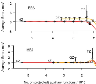
and improves both accuracy and performance dramatically. Accuracy is

enhanced by introducing a Coulomb metric attenuated by a complementary error function

in the resolution-of-the-identity (cf. sec. 3.7), and performance is improved by pivoted

Cholesky decomposition of density-like matrices (cf. sec. 3.2).

Article

II

(page 55) describes a novel method for the generation and compression of

auxiliary bases in resolution-of-the-identity calculations, specifically correlation energy

calculations which require the use of particle-hole pair interactions, such as second-order

Møller–Plesset perturbation theory and the random phase approximation.

Aside from the molecular correlation energy, calculation of molecular properties (cf.

sec. 2.2) is another important field of quantum chemistry. Articles

III

(page 79) and

IV

(page 91) are concerned with the calculation of second-order molecular properties at the

self-consistent field level of theory. Because second- and higher-order must normally be

calculated as derivatives of the electronic energy, computational cost is prohibitive in many

cases. Explicitly using the locality of the perturbing operators (cf. sec. 3.6) to obtain sparse

matrix representations has enabled the calculations of harmonic vibrational frequencies

with

O

(N

)

scaling (page 91), and the calculation of indirect nuclear spin–spin coupling

constants with

O

(

1

)

scaling (page 79), both at the (hybrid-) density functional level of

theory.

2 Theory

2.1 Self-Consistent Field Methods

Hartree–Fock

and Kohn–Sham

theories are two of the most commonly employed

methods for electronic structure calculations. Both provide approximate solutions to the

Schrödinger equations by transforming the many-electron problem to a set of effective

electron problems, where the electron-electron interaction is folded into an effective

one-electron potential. This potential is itself a dependent on the one-one-electron wave functions.

The solutions and potential are iteratively refined until they are self-consistent, i. e., the

one-electron wave function solution set gives rise to the same potential (“field”) as was

used to obtain the wave functions. Hence the term self-consistent field (SCF) theory.

I will review Hartree–Fock and Kohn–Sham theory only very briefly in the following,

noting that countless textbooks are available on the topic (for example refs. 8,43–45). The

aim here is to provide some context to the equations in the following sections and establish

a consistent notation, without reiterating too much textbook knowledge.

2.1.1 Hartree–Fock Theory

Hartree–Fock theory starts with the exact, non-relativistic molecular Hamiltonian ˆ

H

ˆ

H

=

−

X

A

1

2m

∇

2

A

−

X

i

1

2

∇

2

i

+

X

B>A

Z

Z

r

−

X

i A

Z

r

+

X

j>i

1

r

,

(2.1.1)

(in atomic units), where

A

,

B

index nuclei with mass

m

, charges

Z

,

Z

, and

i

,

j

index

elec-trons.

r

=

r

−

r

denotes the distance between particles

x

, y

. The Born–Oppenheimer

approximation is assumed, and the ansatz for the molecular wave function is a single Slater

determinant

|

Ψ

i

built from an orthonormal set of molecular orbitals

|

ϕ

i

(MOs,

one-particle wave functions). The Hartree–Fock energy expression is the expectation value of

the exact Hamiltonian with this Slater determinant:

E

=

h

Ψ

|

H

ˆ

|

Ψ

i

h

Ψ

|

Ψ

i

.

(2.1.2)

This expression is variationally minimized by forming the functional derivative with respect

to the molecular orbitals

|

ϕ

i

and finding the roots of the resulting expression, which yields

the Hartree–Fock equations (canonical form)

ˆ

with

ˆ

F

=

h

ˆ

+

v

ˆ

,

(2.1.4)

ˆ

h

=

−

1

2

∇

2

₊

_v

ext

(

r

)

(2.1.5)

ˆ

v

=

J

ˆ

−

K

ˆ

,

(2.1.6)

ˆ

J

=

X

j

d

r

ϕ

(

r

)

1

|

r

−

r

|

ϕ

(

r

0

₎

₌

_d

_r

ρ

(

r

)

|

r

−

r

|

,

(2.1.7)

ˆ

K

=

X

j

d

r

ϕ

(

r

)

P

|

r

−

r

|

ϕ

(

r

0

₎

_.

_(2.1.8)

The external potential

v

includes the field generated by the nuclei, and possibly other

external fields. The non-local Fock potential ˆ

v

comprises the classical electron-electron

interaction in the Coulomb operator ˆ

J, and the non-classical exchange interaction in the

exchange operator ˆ

K. The permutation operator

P

in Eq. 2.1.8 exchanges the electronic

coordinates

r

and

r

.

Equation 2.1.2 leads to the definition of the correlation energy

E

, which is just the

difference between the exact energy and the Hartree–Fock energy

E

=

E

−

E

.

(2.1.9)

2.1.2 Kohn–Sham Theory

Kohn–Sham theory builds on the Hohenberg–Kohn theorems

to construct an

approx-imate one-electron potential analogous to the Fock potential ˆ

v

(Eq. 2.1.6), called the

Kohn–Sham potential

v

. Unlike the Fock potential, the Kohn–Sham potential is a

func-tional of the electron density

ρ

rather than the molecular orbitals

|

ϕ

i

. Analogously to the

Hartree–Fock equations (2.1.3), the Kohn–Sham equations read

ˆ

F

_|

ϕ

i

=

ε

|

ϕ

i

,

(2.1.10)

ˆ

F

=

−

1

2

∇

2

₊

_v

ext

(

r

)

+

v

(

r

)

,

(2.1.11)

v

(

r

)

=

d

r

ρ

(

r

)

|

r

−

r

|

+

v

(

r

)

,

(2.1.12)

v

(

r

)

=

δ

E

ρ

δ ρ

(

r

)

.

(2.1.13)

Compared to the Hartree–Fock equations, the exchange operator is replaced by the

exchange-correlation (XC) potential

v

(

r

)

, which is the functional derivative of the

exchange-correlation energy functional

E

ρ

with respect to the density

ρ

(

r

)

. While the exact

form of

E

ρ

is unknown for the general case, various constraints and physical insights

As the name suggests, exchange-correlation functionals attempt to fold exchange and

correlation effects into the effective potential. This is in contrast to Hartree–Fock theory,

which only incorporates exchange effects and—by definition—no electron correlation.

2.1.3 Roothaan–Hall Equations

The Hartree–Fock and Kohn–Sham equations are most often (but not exclusively) solved by

expanding the molecular orbitals

|

ϕ

i

in some (generally non-orthogonal) one-electron

basis set

|

µ

_i

|

ϕ

i

=

X

µ

|

µ

_i

C

,

(2.1.14)

which when inserted into Eqs. 2.1.3 or 2.1.10 yields the Roothaan–Hall

equations

X

ν

F

C

=

X

ν

S

C

ε

(2.1.15)

F

=

h

µ

F

ˆ

ν

i

,

(2.1.16)

S

=

h

µ

|

ν

i

,

(2.1.17)

which is simply the matrix representation of the Hartree–Fock or Kohn–Sham equations

in the basis

|

µ

_i

,

_|

ν

_i

, . . .

. Many different types of basis sets are in use, including but not

limited to plane waves and augmented plane waves, wavelets, atom-centered Gaussian or

Slater functions modeled after atomic orbitals (AOs). The results presented in this work,

particularly in chapter 3 and articles

I

-

IV

, used Gaussian functions exclusively. However,

many of the principles are directly applicable to any other type of local basis set. In the

following,

i

,

j

, . . .

will be used for occupied MOs,

a

,

b

, . . .

will be virtual MOs, and

{

p

,

q

, . . .

will be general (occupied or virtual) MOs.

2.1.4 Density Matrix Formulations

It is very often convenient to work with reduced one-particle density matrices instead

of molecular orbitals. For AO-based linear-scaling SCF theories, this is in fact required,

because the canonical molecular orbitals offer no locality. Section 3.3 discusses this aspect

in more detail.

In SCF-type calculations, the density operator is

ˆ

ρ

=

X

p

|

ϕ

_i

n

h

ϕ

|

,

(2.1.18)

where the occupation numbers

n

are zero (virtual orbitals) or unity (occupied orbitals) for

pure states, such as all states considered in this work. The atomic orbital representation of

the density operator in SCF theories reduces to

P

=

X

i∈occ

which is the dyadic product of all occupied MO coefficient vectors

C

P

=

C C

.

(2.1.20)

For pure states, the density operator is a projection operator. Later, it will be useful to define

a “virtual” density, which is the complement of the density (operator), defined by

Q

=

C C

=

S

−

P

,

(2.1.21)

where

C

are the virtual MO coefficient vectors.

Using density matrices in the atomic orbital basis, the energy expression in Hartree–Fock

and Kohn–Sham theories become

E

=

X

µν

P

h

+

1

2

P

G

(

P

)

+

V

(2.1.22)

=

Tr

Ph

+

1

2

PG

(

P

)

!

+

V

,

(2.1.23)

where

V

is the nuclear repulsion energy, and

G

(

P

)

is the matrix representation of the

Fock (Eq. 2.1.6) or Kohn–Sham (Eq. 2.1.12) potential, respectively. This notation shows

the explicit dependence of the effective potential

G

on the density matrix

P

.

2.2 Molecular Properties

Apart from energies, prediction of molecular properties is of high relevance. Predictions

can aid in interpretation of experimental data, substantiate or challenge hypotheses.

For virtually all molecular electronic structure methods, gradients of the energy with

respect to nuclear coordinates are among the most important properties. They allow

opti-mization of molecular geometries toward points of zero gradients, i. e. stationary points on

the potential hyper surface. Other properties accessible include harmonic and higher-order

vibrational frequencies including infrared and Raman intensities, nuclear magnetic

shield-ings tensors, indirect nuclear spin-spin coupling tensors, static and dynamic polarizabilities

and hyper-polarizabilities,

g

-tensors, hyperfine coupling constants.

Some molecular properties can be calculated as simple expectation values of the

ground-state wave function or (spin) densities, for example dipole moments, or hyperfine coupling

constants. Higher-order properties, such as the gradient (first-order) or vibrational

frequen-cies (second-order) are more involved.

2.2.1 Hellmann–Feynman Theorem

with the operator derivative, but no wave function derivatives:

E

=

h

Ψ

_|

_H

ˆ

_|

_Ψ

_i

_(2.2.1)

dE

d

λ

=

h

d

d

λ

Ψ

|

H

ˆ

|

Ψ

i

+

h

Ψ

|

d

d

λ

H

ˆ

|

Ψ

i

+

h

Ψ

|

H

ˆ

|

d

d

λ

Ψ

i

(2.2.2)

=

E

h

d

d

λ

Ψ

|

Ψ

i

+

E

h

Ψ

|

d

d

λ

Ψ

i

+

h

Ψ

|

d

d

λ

H

ˆ

|

Ψ

i

(2.2.3)

=

E

d

d

λ

h

Ψ

|

Ψ

i

+

h

Ψ

|

d

d

λ

H

ˆ

|

Ψ

i

(2.2.4)

=

h

Ψ

_|

d

d

λ

H

ˆ

|

Ψ

i

.

(2.2.5)

While the theorem holds only for complete bases and is therefore typically not applicable

in quantum chemistry, it can still provide valuable insight. In the context of linear-scaling

computation of vibrational frequencies as second-order energy derivatives with respect to

nuclear coordinates, the decay behavior of the interaction can be inferred to be more rapid

than cursory examination suggests. Details of this will be discussed in sec. 3.6. In most

practical calculations, energy derivatives are not evaluated through the Hellmann–Feynman

theorem, but by explicitly computing the derivatives of the energy expression of the method

in question.

2.2.2 Derivatives of the SCF Energy

The first derivative of the Hartree–Fock or Kohn–Sham energy

in a density

matrix-based form (Eq. 2.1.23) with respect to a general perturbation

λ

(we use the shorthand

d

dλ

Z

=

Z

) yields

dE

d

λ

=

d

d

λ

Tr

Ph

+

1

2

PG

(

P

)

!

+

d

d

λ

V

(2.2.6)

=

Tr

Ph

+

1

2

PG

λ

₍

P

)

+

P

(

h

+

G

(

P

))

!

+

V

(2.2.7)

=

Tr

Ph

+

1

2

PG

λ

₍

_P

₎

₊

_P

_F

!

+

V

(2.2.8)

=

Tr

Ph

+

1

2

PG

λ

₍

_P

₎

₋

_WS

!

₊

_V

NN

,

(2.2.9)

with

W

=

PFP

. The identity Tr

P

F

=

−

Tr

WS

can be understood from inspection

of the subspace projections of

P

and

F

:

PSP

SP

=

P

=

−

PS

P

,

(2.2.10)

PSP

(

1

−

SP

)

=

P

,

(2.2.11)

(

1

−

PS

)

P

P

=

P

,

(2.2.12)

Brillouin’s theorem requires that the occupied-virtual and virtual-occupied subspace

pro-jections of

F

vanish. Hence, the only subspace shared between

F

and

P

is the

occupied-occupied space. The first energy derivative may therefore be evaluated without having to

resort to any explicit density or wave function derivatives. This is in accordance with the

Hellmann–Feynman theorem (Eq. 2.2.5) and Wigner’s

(

2n

+

1

)

rule.

For second derivatives, however, a density response is required. The general expression

is

d

E

d

ξ

d

λ

=

d

d

ξ

Tr

Ph

λ

+

1

2

PG

λ

₍

P

)

−

WS

!

+

d

d

ξ

V

NN

(2.2.14)

=

Tr

Ph

+

1

2

PG

λξ

₍

_P

₎

₋

_WS

!

(2.2.15)

+

Tr

P

h

+

P

G

(

P

)

−

W

S

+

V

.

(2.2.16)

Evidently, the density response (or perturbed density)

P

is required for second derivatives,

and may be obtained through solution of the coupled-perturbed SCF (CPSCF) equations,

discussed in sec. 2.2.3.

2.2.3 Coupled-Perturbed SCF

Differentiation of the Roothaan–Hall equations (2.1.15) with respect to perturbation

ξ

yields

X

ν

F

C

+

F

C

=

X

ν

S

C

ε

+

S

C

ε

+

S

C

ε

.

(2.2.17)

Inserting

C

=

P

C

U

and multiplying by

P

C

from the left gives

X

aµν

C

aµ

F

C

+

C

F

C

U

=

X

aµν

C

aµ

S

C

ε

+

C

S

C

U

ε

,

(2.2.18)

or equivalently

F

+

ε

U

=

S

ε

+

U

ε

.

(2.2.19)

After rearranging terms, we obtain a compact form of the coupled-perturbed SCF (CPSCF)

equations

U

=

S

ξ

ai

ε

−

F

ε

−

ε

,

(2.2.20)

P

=

X

ai

C

U

ai

C

+

X

ia

C

U

ia

C

−

X

λσ

P

S

λσ

P

.

(2.2.21)

2.2.4 Laplace-Transformed Density Matrix-Based CPSCF

A transformation of Eq. 2.2.20 to the AO basis has been introduced by Beer and

Ochsen-feld

by means of the the well-established Laplace transformation

1

ε

−

ε

=

0

dt

e

_(2.2.22)

'

τ

X

α=1

w

e

,

(2.2.23)

which is used in Møller–Plesset perturbation theory,

CPSCF,

and in a

differ-ent form in the random phase approximation.

In the context of CPSCF, Eq. 2.2.20 is

rewritten as

U

ai

'

τ

X

α=1

w

e

S

ai

ε

−

F

e

_(2.2.24)

=

τ

X

α=1

w

e

S

ε

₋

F

e

_,

_(2.2.25)

where

ε

is arbitrary. Ayala and Scuseria

pointed out that setting

ε

to a value between

ε

and

ε

(the highest occupied and lowest unoccupied orbital energies,

respec-tively) means the exponential factor is always smaller than unity. We will make use of this

in sec. 3.2.

The density matrix-based Laplace-transformed CPSCF equations introduced by Beer

and Ochsenfeld

read

P

=

X

α=1

Q

−

h

−

G

f

P

g

P

,

(2.2.26)

P

µν

=

√

w

X

i

C

exp

(t

ε

)

C

,

(2.2.27)

Q

µν

=

√

w

X

a

C

exp

(

−

t

ε

)

C

.

(2.2.28)

We refer to

P

and

Q

loosely as “pseudo-density matrices”. Like the regular

one-particle density matrices

P

and

Q

=

S

−

P

, they become sparsely populated for molecular

systems of sufficient size and non-zero band gap.

2.3 Resolution-of-the-Identity

In the context of quantum chemistry, the resolution-of-the-identity (RI)

is used to

approximate four-center two-electron repulsion integrals (ERIs) over atomic basis functions

of the form

µν

_|

λσ

=

d

r

d

r

µ

(

r

)

ν

(

r

)

1

|

r

−

r

|

λ

r

as

µν

_|

λσ

_≈

X

PQ

µν

_|

P

(P

_|

Q)

(Q

_|

λσ

)

,

(2.3.2)

µν

_|

P

=

d

r

d

r

µ

(

r

)

ν

(

r

)

1

|

r

−

r

|

P

r

0

_,

_(2.3.3)

where we introduced the shorthand notation

(P

|

Q)

_≡

_C

PQ,

(2.3.4)

C

=

(P

|

Q)

=

d

r

d

r

P

(

r

)

1

|

r

−

r

|

Q

r

0

_,

_(2.3.5)

and

P

,

Q

are elements of an auxiliary basis set, which is typically about three times as big

as the atomic orbital basis set. RI is also known as “Density Fitting”, because derivation of

Eq. 2.3.2

proceeds by fitting an auxiliary density ˜

ρ

to the exact density

ρ

,

ρ

(

r

)

=

X

µν

µ

(

r

)

ν

(

r

)

P

≈

ρ

˜

(

r

)

=

X

P

χ

(

r

)

C

,

(2.3.6)

and minimizing the residual self-repulsion

R

R

=

d

r

d

r

ρ

˜

−

ρ

₍

_r

₎

˜

ρ

₋

ρ

(

r

)

|

r

−

r

|

.

(2.3.7)

Equation 2.3.2 has been the ubiquitous form of RI for some time. It is used to approximate

ERIs in Kohn–Sham,

Hartree–Fock,

second-order Møller–Plesset,

as

well as coupled-cluster theories.

However, Eq. 2.3.2 is only uniquely defined through Eq. 2.3.7. Alternatively, minimizing

the norm

δ

2

=

d

r

µν

(

r

)

−

X

χ

(

r

)

C

(2.3.8)

leads to

µν

_|

λσ

_≈

X

PQRS

µν

P

(PQ)

(Q

_|

R) (

RS)

(S

λσ

)

,

(2.3.9)

with

(PQ)

_≡

_S

PQ

,

(2.3.10)

S

=

d

r

P

(

r

)

Q

(

r

)

,

(2.3.11)

µν

P

=

d

r

µ

(

r

)

ν

(

r

)

P

(

r

)

.

(2.3.12)

“RI-V”), while Eq. 2.3.9 corresponds to the overlap-metric RI (or “RI-SVS”). In the limit of

a complete auxiliary basis, any metric will give the correct result. In finite bases, Eq. 2.3.2

has been found to yield superior accuracy,

which is why it was universally adopted.

Coulomb-metric RI has a distinct disadvantage compared to overlap-metric RI, however.

In the context of linear-scaling techniques, the three-center two-electron integrals (Eq. 2.3.3)

offer only limited useable sparsity (cf. sec. 3.3) in their atomic orbital representations. In

local bases (e. g., Gaussian functions), the product vector

|

µν

)

vanishes if

|

µ

)

and

|

ν

)

are

centered on points sufficiently far apart. This criterion is universally used in all programs

using local basis functions for virtually all integral evaluations, and it is also useful in the

evaluation of Eq. 2.3.3. However, the

coupling between bra and ket in

µν

_|

P

means

whenever

|

µν

)

is significant, the integral

µν

_|

P

will also be significant. In other words,

the number of significant Coulomb-metric three-center RI integrals grows as

O

(N

)

. In

contrast, overlap-metric three-center integrals offer extremely high useable sparsity, since

the integral decays exponentially in the distance of bra and ket.

Overlap-metric RI was reintroduced by Schurkus and Ochsenfeld

for an effective

linear-scaling RPA algorithm within the RI approximation. Techniques to combine the

advantages of overlap- and Coulomb-metric RI is discussed in article

I

(page 43) and

sec. 3.7.

2.4 Correlation Energies from the Random Phase

Approximation

The Random Phase Approximation (RPA) originates in a series of publications by Bohm

and Pines.

Langreth and Perdew

first defined the RPA correlation energy. In

modern electronic structure literature, the RPA correlation energy is most often derived

from the adiabatic connection

and the fluctuation-dissipation theorem.

Here, we

follow Eshuis

et al.

for the first steps.

2.4.1 Adiabatic Connection Correlation Energy

A well-known result from the adiabatic connection formalism for the correlation energy

E

is

E

=

0

d

α

_h

Ψ

_V

ˆ

Ψ

i − h

Ψ

V

ˆ

Ψ

α=0 0

i

,

(2.4.1)

where

α

is the coupling strength,

Ψ

is the ground-state wave function at coupling strength

α

,

and ˆ

V

is the exact electron-electron interaction. In second quantization, ˆ

V

may be

rewrit-ten as

ˆ

V

=

1

2

X

pqrs

with the creation

c

ˆ

and annihilation

c

ˆ

operators. In terms of the two-particle density

operator ˆ

P

(x

,

x

)

,

ˆ

V

=

dx

dx

ˆ

P

(x

,

x

)

|

r

−

r

|

=

dx

dx

P

ˆ

(x

,

x

)

v

(

x

,

x

)

,

(2.4.3)

where

x

=

(

r

, σ

)

is a combined spin-space coordinate and

v

(x

,

x

)

=

1

/

|

r

−

r

|

is the

bare Coulomb interaction. Using electron field operators

ˆ

ψ

(

x)

=

X

φ

(x)

c

ˆ

,

(2.4.4)

the two-particle density operator reads

ˆ

P

(x

,

x

)

=

1

2

ψ

ˆ

†

_(x

1

)

ψ

ˆ

(

x

)

ψ

ˆ

(x

)

ψ

ˆ

(x

)

,

(2.4.5)

which may be factorized as

ˆ

P

(x

,

x

)

=

1

2

ˆ

ρ

(x

)

ρ

ˆ

(x

)

−

δ

(x

−

x

)

ρ

ˆ

(x

)

,

(2.4.6)

using the fermionic anti-commutator relations

f

ˆ

ψ

(x

)

,

ψ

ˆ

(x

)

g

+

=

δ

(x

−

x

)

,

(2.4.7)

f

ˆ

ψ

(x

)

,

ψ

ˆ

(x

)

g

+

=

f

ˆ

ψ

(x

)

,

ψ

ˆ

(x

)

g

+

=

0

.

(2.4.8)

Introducing the density-fluctuation operator

∆

ρ

ˆ

(x)

=

ρ

ˆ

(x)

₋

ρ

(

x)

,

(2.4.9)

equation 2.4.6 becomes

ˆ

P

(

x

,

x

)

=

1

2

_∆

ˆ

ρ

(

x

)

∆

ρ

ˆ

(x

)

+

ρ

ˆ

(x

)

ρ

(x

)

+

ρ

(x

)

ρ

ˆ

(x

)

−

δ

(x

−

x

)

ρ

ˆ

(x

)

.

(2.4.10)

Inserting Eqs. 2.4.3 and 2.4.10 into the correlation energy expression from the adiabatic

connection (Eq. 2.4.1) leaves just

E

=

1

2

0

d

α

dx

dx

"

_h

_Ψ

0

|

∆

ρ

ˆ

(x

)

∆

ρ

ˆ

(

x

)

|

Ψ

i

|

r

−

r

|

−

h

Ψ

α=0

0

|

∆

ρ

ˆ

(x

)

∆

ρ

ˆ

(x

)

|

Ψ

i

|

r

−

r

|

#

because all other terms vanish identically for

Ψ

and

Ψ

0

. Inserting the

resolution-of-the-identity

1

=

X

n

|

Ψ

_{i h}

Ψ

_|

(2.4.12)

between

∆

ρ

ˆ

(x

)

and

∆

ρ

ˆ

(

x

)

yields

E

=

1

2

0

d

α

dx

dx

X

n

"

_h

_Ψ

0

|

ρ

ˆ

(x

)

|

Ψ

n

i h

Ψ

|

ρ

ˆ

(

x

)

|

Ψ

i

|

r

−

r

|

−

h

Ψ

α=0

0

|

ρ

ˆ

(x

)

|

Ψ

n

i h

Ψ

|

ρ

ˆ

(x

)

|

Ψ

i

|

r

−

r

|

#

.

(2.4.13)

Written more compactly,

E

=

1

2

0

d

α

dx

dx

X

n

f

ρ

(x

)

ρ

(x

)

v

(x

,

x

)

−

ρ

(x

)

ρ

(x

)

v

(x

,

x

)

g

,

(2.4.14)

with

ρ

(x

)

=

h

Ψ

_|

ρ

ˆ

(x)

_|

Ψ

_i

.

(2.4.15)

2.4.2 Frequency Integration of the Polarization Propagator

Next, we inspect the Lehmann representation of the (retarded) polarization propagator

at coupling strength

α

χ

(x

,

x

, ω

)

=

lim

X

n

ρ

(x

)

ρ

(x

)

ω

₋

Ω

+

i

η

−

ρ

(

x

)

ρ

(x

)

ω

+

Ω

+

i

η

!

,

(2.4.16)

which has first-order poles at

z

=

Ω

−

i

η

and

z

=

−

Ω

−

i

η

with residues

Res

χ

(x

,

x

,

z)

|

=

ρ

α

0n

(x

)

ρ

0n

(x

)

,

(2.4.17)

Res

χ

(x

,

x

,

z)

|

=

−

ρ

α

0n

(x

)

ρ

0n

(x

)

.

(2.4.18)

Using Cauchy’s residue theorem, integration along the imaginary axis can be performed by

counter-clockwise integration along the contour

Γ

enclosing

z

, yielding

−∞

du

χ

(x

,

x

,

iu)

=

Γ

dz

χ

(x

,

x

,

z)

(2.4.19)

=

2

π

i Res

χ

(x

,

x

,

z)

|

(2.4.20)

Inserting this result in Eq. 2.4.14 gives a useful expression for the correlation energy

E

=

−

1

4

π

Im

0

d

α

−∞

du

dx

dx

f

χ

(x

,

x

,

iu)

−

χ

(

x

,

x

,

iu)

g

v

(x

,

x

)

,

(2.4.22)

known as the adiabatic-connection fluctuation-dissipation-theorem correlation energy.

2.4.3 Dyson Equation and the Random Phase Approximation

We switch to matrix notation, where multiplication is understood to mean

(

ab

)

=

X

x00

a

b

(2.4.23)

=

dx

_{a x}

_,

_x

_{b x}

_,

_x

_.

_(2.4.24)

The polarization propagator

χ

at coupling strength

α

obeys a Dyson- or

Bethe–Salpeter-type equation

χ

(x

,

x

, ω

)

=

χ

(x

,

x

, ω

)

+

dx

dx

χ

x

,

x

, ω

f

αv

x

,

x

+

f

x

,

x

, ω

g

χ

x

2

,

x

, ω

,

(2.4.25)

or

χ

(

ω

)

=

χ

(

ω

)

+

χ

(

ω

)

f

α

v

+

f

(

ω

)

g

χ

(

ω

)

,

(2.4.26)

where

f

is the (frequency-dependent) exchange–correlation kernel at coupling strength

α

.

The (direct) random phase approximation simply omits

f

so that Eq. 2.4.26 becomes

χ

α

(

ω

)

=

χ

(

ω

)

+

α

χ

(

ω

)

vχ

(

ω

)

,

(2.4.27)

which may be rearranged to

χ

(

ω

)

=

f

χ

0

(

ω

)

−

α

v

g

,

(2.4.28)

where the coupling-strength integral may be evaluated analytically

0

d

α

Tr

χ

(

ω

)

v

=

0

d

α

Tr

_f

χ

0

(

ω

)

−

α

v

g

v

(2.4.29)

=

−

Tr ln

1

−

χ

(

ω

)

v

.

(2.4.30)

Combining this result with 2.4.22 yields a definition of the RPA correlation energy

E

C

=

1

4

π

Im

−∞

du

3 Additional Results

This chapter includes additional results and remarks not included in articles

I

-

IV

.

3.1 The Pivoted Cholesky Factorization for DL-CPSCF

Both the occupied (

P

)and virtual (

Q

) pseudo-densities are positive semi-definite and

therefore amenable to a pivoted Cholesky factorization:

P

=

√

w

exp

(t

PF

)

P

=

P

˜

P

˜

,

(3.1.1)

Q

=

√

w

exp

(

−

t

QF

)

Q

=

Q

˜

Q

˜

.

(3.1.2)

The occupied matrices have rank

N

, and the virtual matrices have rank

N

. The Cholesky

factors

P

˜

and

Q

˜

consequently have dimension

N

×

N

and

N

×

N

,

respec-tively. The canonical DL-CPSCF equation (2.2.26) can be rewritten using the Cholesky

factors as

P

=

τ

X

α=1

˜

Q

Q

˜

−

h

−

G

f

P

g

P

˜

P

˜

.

(3.1.3)

This expression was first given by the author in articles

III

(page 79) and

IV

(page 91).

Because not all matrices here are square, the order of multiplications is important to

performance. The optimum sequence depends on matrix sparsity, as well as the ratio of

occupied to virtual orbitals. We will omit discussion of linear dependencies in the atomic

orbital basis, because they are easily eliminated by projection, and reduce the total number

of molecular orbitals only by a small fraction over the number of atomic orbitals.

In typical calculations with basis sets of useful size (i. e. non-minimal bases), the number

of occupied orbitals is much smaller than the total number of orbitals. We will assume

N

=

N

(and therefore

N

=

N

) in the following, which can be considered

typical for basis sets of double-

ζ

quality.

In the limiting case where all matrices are densely filled, evaluation of Eq. 2.2.26

re-quires 2N

basis

multiplications per Laplace point

α

. The optimal strategy for evaluation of

computational time 6

×

. Performing the Cholesky factorization also on

Q

increases the

number of multiplications to 0

.

38N

basis

.

This discussion typically also holds for sparse matrices. In many cases, however,

factoriz-ing both

Q

and

P

does turn out to be superior after all. This is due to rank reductions

beyond

N

and

N

, discussed in sec. 3.2.

3.2 Rank Reduction Through Cholesky Factorization

For a fixed number of integration nodes

τ

in Eq. 3.1.3, the sum of the numerical ranks of

all

Q

becomes smaller the smaller the HOMO-LUMO gap gets. This follows from the

numerical quadrature of the Laplace-transformed term

. In the interval

x

∈

[1

,

R],

1

x

'

τ

X

α=1

¯

w

exp

(

−

t

¯

x)

.

(3.2.1)

The corresponding roots

w

and weights

t

for the interval

y

=

Ax

∈

[

A

,

B] with

B

=

AR

are

1

y

'

τ

X

α=1

w

exp

−

t

y

,

(3.2.2)

w

=

w

¯

/

A

,

(3.2.3)

t

=

t

¯

/

A

.

(3.2.4)

In this particular application, the quadrature interval is

y

_∈

f

ε

−

ε

, ε

−

ε

g

,

(3.2.5)

where

ε

and

ε

are the HOMO and LUMO energies, respectively, and

ε

and

ε

are the overall highest and lowest MO energies, respectively. For closing

HOMO-LUMO gaps, therefore,

t

in Eq. 3.2.2 grows and the numerical rank of

Q

in Eq. 2.2.28

shrinks.

This means, for instance, that the pivoted Cholesky decomposition provides larger rank

reductions for non-hybrid KS calculations than for HF calculations (for a fixed number

of nodes

τ

), since the former generally produces smaller gaps. In turn, the integration

interval

y

in HF calculations is smaller than in KS calculations, meaning fewer quadrature

points

τ

may be sufficient.

The numerical properties of the Cholesky factorization are discussed in Ref. 100. In

LAPACK (routine

dpstrf

), accuracy is controlled by a tolerance parameter. We have

however, forcing the numerical rank to be just 10 % below the rank revealed by the default

tolerance leads to unacceptable errors.

As a general rule, numerical results are improved when performing the orbital energy shift

(Eq. 2.2.25) discussed in sec. 2.2.4. This is particularly true when using loose tolerances. In

exact arithmetic,

ε

in Eq. 2.2.25 can be chosen arbitrarily. In double precision arithmetic,

however, shifting the orbital energies by as little as

±

5 Hartree leads to severe numerical

instabilities. Thus, we always choose

ε

=

(

ε

+

ε

)

/

2, which means all occupied

MO energies will be negative, and all virtual MO energies will be positive. Consequently,

the argument to the exponential function in Eqs. 2.2.27 and 2.2.28 is always negative, and

numerical singularities are avoided.

In AO-RPA calculations, derivatives of pseudo-density matrices must be evaluated. In

ω

-CDD-RPA (article

I

, page 43), these matrices are Cholesky-factorized. Particularly in

pure (non-hybrid) Kohn–Sham calculations, which form the basis of an RPA calculation, a

few low-lying virtual orbitals with negative orbital energies are the norm rather than the

exception. In such a case, the spectral representation of a virtual pseudo-density matrix

derivative

−

_∂

∂

_t

α

Q

=

√

w

X

a

C

ε

exp

(

−

t

ε

)

C

(3.2.6)

reveals the matrix is manifestly not positive semi-definite and hence not amenable to

Cholesky factorization, unless all virtual orbital energies are shifted to positive values.

Articles

III

(page 79) and

IV

(page 91) established that performing Cholesky-factorizing

the virtual pseudo-density matrices in addition to their occupied counterparts can increase

performance and improve numerical stability, particularly when using sparse algebra. This

is despite the fact that the theoretical number of multiplications increases, as discussed in

sec. 3.1.

3.3 Useable Matrix Sparsity

The key difficulty in the design and implementation of low-scaling variants of

ab initio

theories in the atomic orbitals lies in the matrix sparsity of relevant quantities. It is well

known that the overlap, Fock, and density matrices become sparsely populated—in a local

basis (such as Gaussian functions)—for molecules of sufficient size with non-vanishing

band gaps.

The most successful sparse storage format for

ab initio

calculations is the

blocked-compressed sparse row (BCSR) format,

which divides the source matrix into

sub-matrices (typically 100

×

100 in size) and discards all blocks whose matrix norm

is below a numerical threshold. This format allows for matrix multiplications with very

low overhead, because the sub-matrix multiplications are delegated to high-performance

libraries, often supplied by the processor vendor.

The caveat of the BCSR format, however, is that it only works well for banded sparse

matrices (see figure 3.1 on the facing page for examples). If the significant elements of a

matrix are dispersed all over the matrix, effectively all blocks must be allocated, and no

compression is possible with the BCSR format.

This leads to a concept of useable matrix sparsity within AO-based quantum chemical

calculations. The useable sparsity can be measured by, for example, the matrix bandwidth.

An alternative criterion is the percentage of allocated BCSR blocks required for a certain

accuracy.

Designing an AO-based low-scaling quantum chemical algorithm requires that the matrix

operations preserve useable sparsity. This requirement is the key difficulty. It effectively

eliminates the use of eigendecompositions and singular value decompositions in the

algo-rithm, because the eigenvectors and singular vectors of the Fock and SCF density matrices

have no useable sparsity. One highly useful sparsity-preserving matrix factorization is the

Cholesky decomposition, extensively used in this work in articles

I

through

IV

. Two very

important aspects of useable matrix sparsity will be discussed in sections 3.4 and 3.5.

3.4 Sparsity of the Virtual Density Matrix

One of the more common misleading statements in much of the literature concerning the

sparsity of density matrices concerns the virtual density matrix (Eq. 2.1.21 on page 18). It

is true that, for typical molecular calculations using atom-centered Gaussian basis sets, the

contravariant atomic orbital

representation of the virtual density matrix

Q

is much less

sparse than the corresponding occupied density matrix representation. However, Eq. 2.1.21

simplifies to

Q

=

1

−

P

(3.4.1)

when the atomic orbital basis has been orthogonalized. In other words, the occupied and

virtual density matrices have identical sparsity patterns in an orthogonalized basis. There is

no physical reason whatsoever dictating the virtual density matrix be any less local (sparse)

than the occupied density matrix. The confusion arises due to the presence of

S

in

Eq. 2.1.21. In Gaussian orbitals, the overlap matrix

S

is extremely sparse, because elements

S

decay as exp

−

r

_{in the distance}

_r

_{of their centers. Matrix inversion will destroy a}

significant portion (but by no means all) of this sparsity. Hence, in the contravariant AO

basis, the virtual density matrix

Q

is much less sparse than its occupied counterpart

P

.