Towards grid-based O
„
N
…
density-functional theory methods: Optimized nonorthogonal
orbitals and multigrid acceleration
J.-L. Fattebert*and J. Bernholc
Department of Physics, North Carolina State University, Raleigh, North Carolina 27695-8202
共Received 13 September 1999兲
We have formulated and implemented a real-space ab initio method for electronic structure calculations in terms of nonorthogonal orbitals defined on a grid. A multigrid preconditioner is used to improve the steepest descent directions used in the iterative minimization of the energy functional. Unoccupied or partially occupied states are included using a density matrix formalism in the subspace spanned by the nonorthogonal orbitals. The freedom introduced by the nonorthogonal real-space description of the orbitals allows for localization constraints that linearize the cost of the most expensive parts of the calculations, while keeping a fast conver-gence rate for the iterative minimization with multigrid acceleration. Numerical tests for carbon nanotubes show that very accurate results can be obtained for localization regions with radii of 8 bohr. This approach, which substantially reduces the computational cost for very large systems, has been implemented on the massively parallel Cray T3E computer and tested on carbon nanotubes containing more than 1000 atoms.
I. INTRODUCTION
The relative simplicity and accuracy of density-functional theory 共DFT兲has enabled great progress in electronic struc-ture calculations.1,2The fact that the exchange and correla-tion interaccorrela-tions between electrons can be quite accurately described by a potential that depends only on the electronic density and possibly its gradient关the local-density and gen-eralized gradient approximations共LDA兲and共GGA兲, respec-tively兴 is an enormous simplification that led to ab initio calculations for systems containing a fairly large number of atoms. However, the interest in complex and/or technologi-cal materials and structures is stimulating the development of methods that can substantially enlarge the number of atoms that can be handled by DFT techniques.
The largest calculations usually employ pseudopotentials, which eliminate the need to explicitly consider core electrons in the Kohn-Sham共KS兲equations. This enables the descrip-tion of the electronic wave funcdescrip-tions in a plane wave basis, which offers substantial advantages: 共i兲plane waves do not depend on the atomic positions, which simplifies the calcu-lation of the atomic geometry and makes the results more precise, and 共ii兲the accuracy is determined by a single pa-rameter, the highest kinetic energy of the waves included in the calculations. The structure of the DFT equations is also advantageously exploited in the plane-wave basis: the kinetic energy is diagonal in Fourier space, while the potential terms are diagonal in real space. The transformation between the two spaces occurs via the well-known fast Fourier transform 共FFT兲algorithm, which is very fast on vector supercomput-ers and modern workstations. However, its performance slows down on massively parallel computers since FFT is a global operation.
Recently, there has been substantial interest in the so-called real-space methods, which offer the promise of even larger calculations. There are several reasons for this, the most obvious being easier parallelization, since specific re-gions of space could just be assigned to particular
proces-sors. More subtly, multiscale convergence acceleration techniques,3 which can substantially reduce the number of steps in an iterative solution, are usually formulated in real space. Finally, and most importantly for the present article, a real-space formulation is necessary for the implementation of the O(N) techniques, which promise to reduce the asymptotic O(N3) scaling of traditional electronic structure methods with respect to the number of electrons or atoms.
Real-space bases that employ atom-centered functions, e.g., Gaussians or localized atomic orbitals, have long been used in electronic structure calculations. However, large nu-merical bases are also very interesting since they allow one to attain any desired numerical accuracy by systematically increasing the number of degrees of freedom. The numerical bases used in recent calculations include finite elements,4–8 grids,9–17 and wavelets.18–20 These bases allow for natural implementation of mesh refinement,9,11,12,14,15cluster bound-ary conditions, and efficient domain decomposition ap-proaches on massively parallel computers.12,13,15
The computational effort in traditional electronic structure calculations must ultimately scale as O(N3), where N is the number of atoms. This is because the wave function of each electron can, in general, extend over the whole material, and therefore computing one wave function will take at least
O(N) operations. Since the number of electrons grows
lin-early with the number of atoms, the computational effort must grow at least as O(N2). Furthermore, the individual wave functions must be orthogonal to each other and the orthogonalization or diagonalization effort will ultimately dominate, since they scale as O(N3).
Recently, a number of ingenious methods have been pro-posed for evaluating the total energy in O(N) operations. These methods usually make a localization approximation, which involves either the use of a localized, Wannier-like basis21–27or a neglect of off-diagonal elements of the density matrix 共r,r
⬘兲
for 兩r⫺r⬘
兩 greater than an appropriate cutoff radius.28–33In the wave function-based approaches the main idea is to rewrite the total energy expression with the help ofPRB 62
basis functions that are unknown at the outset and are to be variationally optimized in the process of minimizing the total energy. Each function is localized, i.e., confined to a given region in space, but the confinement regions for the various functions overlap. Since overlaps between functions local-ized in regions sufficiently far away vanish, the number of nonzero overlaps is O(N). By exploring this sparsity and avoiding the calculation of individual eigenfunctions, it is possible to evaluate the total energy in O(N) operations. In the density-matrix approaches, when formulated for full density-functional calculations with large numerical bases, it is necessary to expand the density operator in a basis of localized orbitals,34–36in order to reduce its effective dimen-sion. Other methods, based on the divide-and-conquer algorithm,37,38energy renormalization group for the density matrix,39 or calculation of the Green’s function,40 have also been proposed. Recently, fully self-consistent O(N) DFT calculations that used atomiclike orbitals as a basis have been reported.41 A more comprehensive discussion and list of references is given in recent reviews by Galli42 and Goedecker.43
The electronic structure of a physical system is easiest to describe in the basis of eigenfunctions, but any set of func-tions spanning the same subspace is also appropriate. How-ever, if one imposes localization constraints, which require that a given function is zero outside of a prescribed localiza-tion region, these different choices are no more equivalent. When searching for a basis set that most accurately approxi-mates the solution with the localization constraints, it is im-portant to work with a general nonorthogonal basis set. All quantities of interest need to be expressed in this set: the total energy, the steepest descent共SD兲directions, preconditioners, and forces. This excludes the direct use of methods based on the search for the eigenvectors, e.g., Lanczos’, Davidson’s, or inverse iteration methods.
Real-space methods are inherently local, and therefore suitable for imposing localization constraints on the basis functions that span the subspace of the occupied orbitals. In the present paper, we investigate the performance of O(N) techniques in the context of grid-based DFT calculations. Let
N denote the number of wave functions needed and M the
number of points of the grid used to discretize the KS prob-lem. In general, N is much smaller than M. The computa-tional cost for tractable systems is thus dominated by those parts of the algorithm that grow like M⫻N2. These opera-tions usually consist of the construction of N⫻N matrices
共overlap, Hamiltonian, etc.兲 in the basis of the trial wave functions, and the update of the trial wave functions in an orthogonalization or Ritz procedure. This cost can be largely reduced if spatial localization can be imposed on the orbitals that describe the ground state of the system. Localized orbit-als orbit-also reduce the memory requirement, which scales as N ⫻M , in general. Note that when MⰇN, a good
precondi-tioner is also required for an efficient iterative minimization. Otherwise a convergence slowdown would be observed as the system size increases, which would make a nonacceler-ated O(N) method slower than a preconditioned N3 tech-nique.
The method proposed in this paper is closely related to several recently described techniques, particularly that of Galli and Parinello,21 where the Kohn-Sham equations are
rewritten in terms of nonorthogonal, localized orbitals ex-panded in a plane-wave basis. Their basic idea is to use the nonuniqueness of the representation of the ground state of the system in terms of nonorthogonal orbitals to find an op-timally localized basis that accurately describes the electrons. Our approach is more general and real-space oriented: we include a multigrid preconditioner and allow for unoccupied or partially occupied states. Indeed, numerical tests on real-istic systems show that the inclusion of some unoccupied states substantially accelerates convergence. The unoccupied states are included using techniques similar to the density-matrix approach for nonorthogonal orbitals.30,34,35However, we do not impose additional localization constraints on the density matrix for reasons of accuracy and numerical effi-ciency, which results in a small O(N3) part for N⫻N matrix
operations. This approach is efficient for a wide range of system sizes. For example, in our massively parallel imple-mentation on the Cray T3E supercomputer, the O(N3) part does not exceed 20% of the computational cost for systems containing over 1100 atoms 共see Sec. IV兲.
In our real-space calculations on a grid, we use a compact and accurate Mehrstellen finite difference共MFD兲scheme of order 4,44 which has been successfully introduced in elec-tronic structure calculations a few years ago.12,14 It dis-cretizes the entire differential equation, as opposed to the Laplacian, and only uses the first- and second-neighbor points on the three-dimensional grid. As a result, zero bound-ary conditions are easy to impose at the boundaries and the short range of the discretization also aids parallelization. However, while the methodological discussion in this paper explicitly uses the MFD discretization, most of the argu-ments are general and can be applied to any other real-space method. For simplicity, the discussion is also restricted to real wave functions, but extensions to complex wave func-tions and k points are straightforward.
The optimized localized orbitals are also very useful apart from facilitating exceedingly large calculations. They have already enabled efficient calculations of quantum transport properties, which rely on the expansion of Hamiltonian and Green’s function matrices in terms of localized orbitals.45 Since one can use very few short-range localized functions per atom, e.g., three for the case of carbon atoms, the dimen-sions of the relevant matrices are minimized, which has led to ab initio calculations of quantum conductance for large nanotube structures.46
The remainder of this paper is organized as follows. In Sec. II, the general method for minimization of the energy functional in a nonorthogonal basis is described. The multi-grid acceleration scheme and the MFD discretization are also discussed. Section III focuses on the implementation of lo-calization constraints for nonorthogonal orbitals and their ef-fect on the scaling of the calculations. Section IV presents numerical test results for long carbon nanotubes, containing up to 1120 atoms. Some mathematical details are given in the Appendix.
II. GENERAL ITERATIVE ALGORITHM FOR NONORTHOGONAL ORBITALS
A. Basis-invariant matrix formulation
Consider the standard problem of minimizing the Hohenberg-Kohn total energy functional1
Et⫽
兺
j⫽1 Nfj具j兩⫺
1 2ⵜ
2兩j典⫹1
2
冕
VH共兲dr⫹
冕
Vion共兲dr⫹Exc关兴⫹Eion⫺ion 共1兲for N-occupied orbitals in the system, each represented by a one-body wave functionj, with the electron charge density
(r)⫽兺jN⫽1fj兩j(r)兩2. The first term represents the kinetic energy, the second the electrostatic repulsion due to the clas-sical Hartree potential VH(r)⫽兰(r
⬘
)/兩r⫺r⬘
兩dr⬘
, the third the interactions of the electrons with all the nuclei, the fourth the exchange and correlation contributions, and the fifth the classical electrostatic interactions between all nuclei.The orbitalsj satisfy the Kohn-Sham equations 2
Hj⫽关⫺
1 2ⵜ
2⫹V
ion⫹VH共兲⫹xc共兲兴j⫽⑀jj, 共2兲 which must be solved self-consistently for the N lowest ei-genvalues⑀j, while imposing the orthonormality constraints
具
i兩j典⫽␦i j. xc⫽␦Exc关兴/␦ is the exchange and corre-lation potential. Using Eq.共2兲, the total energy expression is easily rewritten asEt⫽
兺
j⫽1 N
fj⑀j⫺1
2
冕
VH共兲dr⫺冕
xc共兲dr⫹Exc关兴⫹Eion⫺ion. 共3兲
In the remainder of this subsection we will assume that each orbital is fully occupied, i.e., fj⬅2.
In practice we use norm-conserving nonlocal pseudopo-tentials in the Kleinman-Bylander form
Vion⫽Vloc⫹Vnl, where
Vnl⫽
兺
i,␣ 兩KBi,␣
典具
KBi,␣兩. 共4兲
The index i refers to the atoms and␣ to the projectors of the nonlocal pseudopotentials.
Consider a trial basis of normalized functions,
兵1, . . . ,N其, that will define the subspace of the occupied orbitals. This basis will be refined by iterative updates, and at convergence will accurately describe the true Kohn-Sham ground state of the system. In order to derive basis-invariant expressions for the updates, it is convenient to use matrix notations. The functions j will thus be written as columns of a matrix⌽
⌽⫽共1, . . . ,N兲.
An orthonormal basis of approximate eigenfunctions 共Ritz functions兲can be obtained by a diagonalization in this sub-space of dimension N共Ritz procedure兲. We denote by C the
N⫻N matrix that transforms⌽into the basis⌿of orthonor-mal Ritz functions,
⌿⫽共1, . . . ,N兲⫽⌽C. 共5兲
This matrix satisfies
CCT⫽S⫺1, where
S⫽⌽T⌽, is the overlap matrix.
In the following, for an operator A we will use the nota-tion
A(⌿)⫽⌿TA⌿,
A(⌽)⫽⌽TA⌽. We then have the relation
A(⌿)⫽CTA(⌽)C.
In order for Eq. 共5兲 to define a transformation to a Ritz basis, C has to be a solution of the generalized symmetric eigenvalue problem
H(⌽)C⫽SC⌳, 共6兲 where⌳ is the diagonal, real N⫻N matrix that satisfies
⌳⫽⌿TH⌿.
The matrix C can actually be decomposed as a product C ⫽G⫺TU, where G is the Cholesky factorization of S,
S⫽GGT,
and U is an orthogonal matrix. Knowing G, the generalized eigenvalue problem 共6兲 is reduced to a standard symmetric eigenvalue problem
G⫺1H(⌽)G⫺TU⫽U⌳. 共7兲 In the basis⌿, the SD directions, along which the energy functional decreases at the fastest rate, are easy to compute. They are given by the negative residuals of the Kohn-Sham equations 共2兲, with the current potential kept fixed, and can be expressed as the N⫻M matrix
D(⌿)⫽⌿⌳⫺H⌿, 共8兲 which satisfies the relation
⌿TD(⌿)⫽0.
In the following, we consider a SD algorithm with a linear preconditioning operator K. Without preconditioning, the convergence rate can be very slow, especially if MⰇN. For
real-space finite difference共FD兲discretizations, the multigrid preconditioner described in Sec. II D greatly improves the convergence. Introducing a pseudo-time-step , ⌿ should thus be corrected at each step according to
⌿new⫽⌿⫹KD(⌿).
Note that in this algorithm all the trial wave functions are updated simultaneously. Without preconditioning, has to be very small 共for numerical stability reasons兲and the con-vergence can be very slow.
nonorthogonal orbitals ⌽. This direction can differ substan-tially from the derivative with respect to j(r) when the basis⌽is highly nonorthogonal. Since the direction D(⌿) is easy to compute, the simplest way to obtain the SD direction in the basis⌽is to use the matrix C
D(⌽)⫽D(⌿)C⫺1⫽共⌿⌳⫺H⌿兲C⫺1
⫽⌽⌰⫺H⌽, 共9兲
where
⌰⫽S⫺1H(⌽). 共10兲
The preconditioned steepest descent 共PSD兲 direction in the nonorthogonal basis is thus
␦⌽⫽KD(⌿)C⫺1
⫽K共⌽⌰⫺H⌽兲, 共11兲
and the basis⌽is updated according to⌽new⫽⌽⫹␦⌽. In the particular case K⫽Identity, Eq.共11兲is equivalent to the result given in Ref. 21. Note that␦⌽does not depend on C and therefore does not require the solution of the eigenvalue problem共6兲.
Note that since by definition
⌽new⫽共⌿⫹KD(⌿)兲C⫺1⫽⌿newC⫺1,
the same subspace is generated at each iteration, indepen-dently of the basis, if the same pseudotime step is used. In principle, the above SD directions could also be used to-gether with a conjugate gradient共CG兲method,47but the con-vergence rate of the preconditioned algorithm described be-low was fast enough, in all applications to date, to make the implementation of the CG approach unnecessary.
In actual calculations, the basis functions⌽are corrected at each iteration using the PSD directions共11兲. A new elec-tronic density(r) is then generated according to
共r兲⫽2
兺
j,k⫽1N
共S⫺1兲jkj共r兲k共r兲,
as well as the new Hartree and exchange-correlation poten-tials. However, the old and the new potentials are then mixed linearly. The functional共1兲is minimized iteratively until self consistency is achieved.
At each step, the kinetic energy Ekin can be evaluated in the nonorthogonal basis ⌽as
Ekin⫽2
兺
j,k⫽1N
共S⫺1兲jk具⌽j兩⫺
1 2ⵜ
2兩⌽k典.
To obtain the ground-state energy Et, the first term on the right-hand side of Eq. 共3兲can be expressed as a trace of⌰,
兺
j⫽1 N2⑀j⫽2 Tr共⌳兲⫽2 Tr共⌰兲.
B. Computations with unoccupied orbitals
We have found that the inclusion of unoccupied or par-tially occupied orbitals substanpar-tially enhances the conver-gence rate共see Sec. IV兲. The PSD algorithm described above
can be used to improve the trial subspace of N computed orbitals, regardless whether they are occupied or empty. In the computation of the electron density and the total energy, however, one needs to account for the occupations. To this end, we introduce a density-matrix formalism in the nonor-thogonal basis.
For a chemical potential, define the N⫻N matrix⌼by its matrix elements
⌼i j⫽␦i jf关共⑀i⫺兲/kBT兴,
where f is a Fermi-Dirac distribution. The density operatorˆ is then given by
ˆ⫽⌿⌼⌿T⫽⌽C⌼CT⌽T.
For T⫽0, the operator ˆ is a projector onto the states of eigenvalues lower than . In a grid-based approach, the di-mension of this discrete density matrix is given by the num-ber of degrees of freedom, i.e., the numnum-ber of points on the real-space grid. This number is, in general, so large that it is impossible to apply iterative methods that require (r,r
⬘
) 共matrix of size M⫻M ). However, one can representˆ in thebasis⌽
(⌽)⫽⌽Tˆ⌽⫽C⫺T⌼C⫺1.
As in Ref. 30, we introduce the matrix¯(⌽)
¯(⌽)⫽S⫺1(⌽)S⫺1⫽C⌼CT. 共12兲
This matrix can be used to obtain the expectation value A¯ of an operator A represented in the basis⌽
A
¯⫽2 Tr共⌼A(⌿)兲⫽2 Tr共¯(⌽)A(⌽)兲.
In particular, the total number of electrons in the system is given by
Ne⫽2 Tr共¯(⌽)S兲.
Note that if all the computed states are fully occupied, we have (⌽)⫽S and¯(⌽)⫽S⫺1.
Using the solution C of the generalized symmetric eigen-value problem 共6兲, one can compute the matrix ¯(⌽) using Eq. 共12兲. The electronic density is then given by
共r兲⫽2
兺
j,k⫽1N
共¯(⌽)兲
jkj共r兲k共r兲. 共13兲
The first term on the right-hand side of Eq. 共3兲, commonly referred to as the band-structure energy, can be computed as
2
兺
j⫽1 N⑀jf关共⑀j⫺兲/kBT兴⫽2 Tr共⌳(⌿)兲
⫽2 Tr共H(⌽)¯(⌽)兲. 共14兲
meth-ods of Refs. 27 and 36, where the rank of the overlap matrix
S decreases to the number of occupied orbitals at
conver-gence.
In the calculations of the forces on the ions, the only term that differs from calculations with eigenfunctions is the one associated with the nonlocal part of the pseudopotential. The energy term for this part is given by
Enl⫽Tr共⌽TVnl⌽¯(⌽)兲.
At present, we obtain the forces on the ions by evaluating a numerical derivative of the energy with respect to the ionic positions. This is done by computing changes in the total energy for small virtual displacements of the ions, without the need for full self-consistent calculations. The associated computational cost is thus insignificant.
C. Mehrstellen finite difference discretization
To compute an approximate numerical solution to the KS equations we use a Mehrstellen finite difference共MFD兲 method. Upon discretization, one obtains a linear algebra eigenvalue problem
H⫽⑀B,
where H and B are real, sparse M⫻M matrices, with M
being the number of points on the real-space grid. The details of the MFD methodology and its implementation on mas-sively parallel computers using domain decomposition are described in Ref. 12.
In the above notation, ⌿ and⌽ denote matrices M⫻N,
the columns of which correspond to the values of wave func-tions on the discretization grid. The steepest descent direc-tions are given by
D(⌿)⫽B⌿⌳⫺H⌿, 共15兲 and
D(⌽)⫽D(⌿)C⫺1
⫽B⌽⌰⫺H⌽, 共16兲
where
⌰⫽共B(⌽)兲⫺1H(⌽).
For the MFD scheme H(⌽) should be replaced in Eqs.共6兲, 共7兲, and共14兲by
HB⫽S共B(⌽)兲⫺1H(⌽).
As shown in the Appendix, HB is a symmetric matrix at convergence. In practice, before reaching convergence, we explicitly symmetrize HB.
In the above approach, the electron density at the point ri is given by
ii⫽2
兺
j,k j共ri兲k共ri兲共¯(⌽)兲jk.
The implementation issues of this algorithm are discussed in Sec. IV.
D. Multigrid preconditioning
Obtaining O(N) scaling for the most expensive parts of the calculations is useful only if its prefactor is not much larger than for O(N3) calculations. It is thus impor-tant to have a preconditioner that works well for nonortho-gonal orbitals. The importance of an efficient preconditioner for electronic structure calculations with large numerical bases has been recognized in Ref. 48, in the context of the plane-wave method. For real-space electronic structure cal-culations several efficient iterative solvers have been devel-oped recently,12,14,16,17,49 based on multilevel acceleration techniques.3 For O(N) methods, the importance of precon-ditioning has recently been discussed in Ref. 50.
A general mathematical analysis of parallel multilevel preconditioners for discretized partial differential equations has been given in Ref. 51. Here we introduce a specific mul-tigrid preconditioner appropriate for electronic structure cal-culations in a nonorthogonal basis. Given a SD direction d, a preconditioned SD direction u⫽Kd is computed. The
opera-tor K represents an iterative multigrid solver (V cycle兲3 for the Poisson equation
⫺1 2ⵜ
2u⫽d, 共17兲
with an initial u given by u0⫽2␣d, and limited to the grids with a number of points larger than N, where Jacobi itera-tions are used as a smoother. The coefficient␣ is an estimate of the smallest eigenvalue of (H⫺⑀j)⫺1on the coarsest grid,
␣⫽ 1
2
4Lh2⫹兩Vmax⫺⑀1兩
,
where L denotes the number of coarse grids used, Vmax the maximum of the total potential, and⑀1the lowest eigenvalue of HB. The role of the preconditioner is to systematically reduce high-frequency components in the SD directions. This preconditioner has the important property that its effi-ciency does not depend on the basis we work in and is very cheap共less than 20% of a self-consistent step兲. Moreover, it can be applied in the same manner to localized or delocal-ized orbitals.
The purpose of the iterative corrections of the wave functions is to reduce as fast as possible the components orthogonal to the subspace one is solving for. Since the above preconditioner deals much better with components as-sociated with the highest eigenvalues of the Hamiltonian than with the ones associated with the lowest eigenvalues— due to the similarity between the eigenfunctions associated with the largest eigenvalues of the Hamiltonian and those of the Laplacian operator—the larger the N the better it works. In practice, taking into account cost and efficiency, it is ad-vantageous to introduce some unoccupied states 共10–30 %兲 in⌽.
However, the use of one or two coarse grids significantly improves the convergence rate at a very low additional cost. The good efficiency of the preconditioner allows us to avoid the conjugate-gradient algorithm, which would largely in-crease the cost per iteration. Note that one self-consistent 共SC兲iteration consists of only one simultaneous PSD correc-tion for all the orbitals, followed by an update of the electron density and the potential. At each iteration, the Poisson equa-tion for the Hartree potential is iteratively solved by a stan-dard multigrid algorithm.
III. LOCALIZATION AND PARTIAL LINEAR SCALING
In the method described above, the removal of the or-thogonalization step has been replaced by a more compli-cated and expensive SD calculation, Eq.共9兲, so that the com-putational cost of the minimization scheme is roughly the same. Furthermore, the calculation of the electron density is much more expensive when using a basis different from Ritz functions, since in the latter case (⌽) becomes diagonal. However, when working with nonorthogonal functions⌽ in-stead of the Ritz functions ⌿, one can easily impose local-ization constraints on⌽to reduce the cost of the calculation. Localization is imposed by forcing the functions to be zero outside of a spherical region centered on an ion. In particular, such truncation will linearize the computational cost of D(⌽) in Eq.共9兲and in Eq.共13兲, the most expensive parts of the algorithm. In addition, the nonorthogonal basis allows for the use of techniques that accelerate convergence for systems with a small band gap, see, e.g., Ref. 52.
The application of the MFD Laplacian operator to a wave function localized in a sphere of radius Rcgenerates a func-tion localized in a sphere of radius Rc⫹h
冑
3, which is used as the localization radius for Hj and Bj. This truncation suppresses some components of Hj that are generated by the nonlocal, short-range projectors of the pseudopotential operator. These components are not used to correct the wave functions since the latter should remain localized. However, they are included exactly in the computation of the matrix⌰ and the total energy by writing H(⌽) as the sum of two ma-tricesH(⌽)⫽⌽T共H⫺BVnl兲⌽⫹⌽TBVnl⌽,
which isolates the nonlocal potential Vnlin the second term. This term can be easily computed in O(N) operations using only the values of (Bj)TKB
i,␣
and (KBi,␣)Tj. Therefore, the only approximation in this approach is the use of a localiza-tion radius to limit the spatial extent of each nonorthogonal orbital.
If unoccupied states are used, both inverses and eigenvec-tors of N⫻N matrices are needed. Since the eigenfunctions
are, in general, not localized, the matrix C that solves Eq.共6兲 is not sparse, and thus the required number of operations is proportional to N3. However, when no partially occupied states are present and an estimate of the chemical potential is available, one can use the method of Refs. 28–30 to com-pute¯(⌽). Specifically, ˆ can be defined as the operator Xˆ that minimizes the functional
⍀关Xˆ兴⫽Tr兵关3共X(⌿)兲2⫺2共X(⌿)兲3兴关共B(⌿)兲⫺1H(⌿)⫺I兴其. 共18兲
This minimum can be computed iteratively by a conjugate gradient algorithm using the true steepest descent directions.53 In the nonorthogonal basis ⌽, defining X¯(⌽) ⫽S⫺1X(⌽)S⫺1, one has to minimize共see Appendix兲
⍀关X¯(⌽)兴⫽Tr关共3X¯(⌽)SX¯(⌽)⫺2X¯(⌽)SX¯(⌽)SX¯(⌽)兲
⫻共HB⫺S兲兴. 共19兲
The localization constraints, X¯i j (⌽)⫽
0 if the localization re-gions of orbitals i and j are separated by a distance larger than a truncation radius R, can be imposed at each step of the iterative minimization in order to achieve linear scaling. This procedure is justified by the exponential decay of
(r,r
⬘
) as 兩r⫺r⬘
兩→⬁ in insulators or metals at a finite temperature.54 However, the matrix elements obtained from Eq. 共19兲 are, in general, not exactly the same one would obtain in an N3 calculation. Moreover, good accuracy can be obtained only by keeping the number of nonzero elements inX
¯ much larger than in S.33,34
When MⰇN, the full evaluation of S⫺1,⌰, or¯(⌽), even with an order N3 algorithm, constitutes a small fraction of the calculations for a large range of system sizes. For ex-ample, in parallel multigrid calculations of Ref. 12, the Cholesky decomposition and the diagonalization of the N ⫻N matrices were not even parallelized, since they
ac-counted for a negligible part of the computational effort for practical system sizes. When using localized orbitals, the maximum practical system size increases substantially, but the cost of the N⫻N matrix operations remains a small
frac-tion of the total for a large range of systems, if these opera-tions are effectively parallelized using standard libraries, such as PBLAS 共Parallel Basic Linear Algebra Subpro-grams兲and ScaLapack.55Table I shows some timings for the Scalapack diagonalization routine used in the O(N3) part of our method. For systems with more than 1000 orbitals, di-agonalization on a single processor becomes very expensive, if required at each self-consistent iteration. However, since the multigrid calculations are fully parallel, it is natural to also parallelize the diagonalization, which substantially
re-FIG. 1. Convergence rate of the multigrid-preconditioned SD for different numbers of grid levels, using the C60molecule as an
duces the elapsed time and thus greatly increases the maxi-mum system size that can be studied at reasonable cost.
In the current calculations, S, H(⌽), ⌰, and ¯(⌽) are stored as full N⫻N matrices, distributed on the processors
according to PBLAS and ScaLapack requirements. Although most of the operations on these matrices can be optimized using their sparsity—except the diagonalization in Eq.共7兲— the full storage approach is adequate for a substantial range of calculations. It is also the easiest to implement given the numerical libraries and the parallel computers we have ac-cess to. The solution of the eigenvalue problem共7兲is clearly the dominant part of these O(N3) operations.
Since the method described above determines the eigen-functions of the Kohn-Sham equations in the basis of local-ized functions, it can be viewed as a generalization of ab
initio methods that use a linear combination of atomic
orbit-als 共LCAO兲 or Gaussians functions G to expand the eigen-functions:⌿j⫽兺iciGi. The main difference is that our local functions ⌽i are defined by their values on a grid and are variationally optimized. In particular, the functions⌽i have many more degrees of freedom and one can systematically increase the accuracy of the calculations by mesh refinement or expansion of the localization domain. The number of basis functions in high-precision calculations can thus be much smaller than in Gaussian or LCAO approaches, which mini-mizes the O(N3) part. Furthermore, since exact and explicit
O(N3) diagonalization is performed, cf. Eq. 共7兲, both par-tially occupied and unoccupied orbitals can be used, which permits calculations for metallic as well as semiconducting systems. However, calculations for metals may require more localized orbitals or larger localization radii for an accurate description. Having a small number of basis functions is also important in other contexts. For example, transfer-matrix-based calculations of quantum transport benefit substantially from the small size of the basis and the optimized functions ⌽ have already been used to evaluate the conductances of carbon nanotubes.46The above approach is also very useful for evaluating the effects of localization constraints alone, while maintaining high local accuracy. However, for very large future calculations the O(N3) terms will eventually dominate, and the formulation 共19兲 may become advanta-geous.
IV. APPLICATIONS TO TEST SYSTEMS
The algorithm described above has been implemented on the massively parallel Cray T3E supercomputer and tested on C60 and carbon nanotubes of varying lengths. Our calcu-lations used the pseudopotentials of Hamann56,57 and the LDA forxc. The pseudopotentials were filtered in order to remove high frequency components that cannot be
repre-sented on the grids employed.12 Periodic boundary condi-tions were used in all cases. The starting trial basis funccondi-tions were atom-centered random functions strongly localized around their respective atoms. In order to improve the con-ditioning of the overlap matrix, the functions localized on the same atom were kept orthonormal during the entire calcula-tion. The initial trial density was a linear combination of atom-centered Gaussians, neutralized by the positive ions. The density also defined the initial potential. To improve stability, the initial potential was kept fixed during the first 2-3 SC iterations. Thereafter, the potential was updated at each step, mixing usually 20–50 % of the current potential with the KS potential associated with the previous density. In our test cases the condition number of the overlap matrix S increased during the iterations, but it remained small enough to ensure stable numerical results.
To take advantage of the localization constraints, several nonoverlapping localized orbitals were stored in the same
global array that represents a function extending throughout
the whole discretization grid. These orbitals can thus be re-laxed simultaneously at the same cost as the relaxation of one spatially extended orbital. In practice, when computing matrix elements between pairs of orbitals, the real-space grid was divided into regular blocks whose contributions were summed up. For this purpose, it is important that only one orbital of each global function is non-zero on each block, so that the contributions can be associated with one and only one orbital. On a massively parallel computer, a block can be a subdomain associated with a processor, or a fraction of this subdomain. The main advantage of the above approach is that it avoids indirect addressing and can efficiently use stan-dard, optimized linear algebra libraries in each block.
As mentioned in Sec. II B, the introduction of unoccupied states in the calculations can substantially improve the con-vergence rate. This effect is illustrated in Fig. 2, which com-pares the convergence rates for C60 when either no or one unoccupied state per carbon atom is included in the calcula-tions. When introducing localization constraints, the inclu-sion of unoccupied states has an even greater effect since these states introduce additional degrees of freedom that par-tially compensate for the localization-induced truncation. In the impractical limit of having as many localized functions as the number of grid points, the localized and nonlocalized
FIG. 2. The effect of unoccupied states on the convergence rate for the case of C60.
TABLE I. Diagonalization times of a typical Hamiltonian ma-trix, using the ScaLapack subroutine PSSYEV, as a function of the number of processing elements共PE’s兲on the Cray T3E.
共s兲 1 PE 4 PE’s 16 PE’s 64 PE’s
N⫽560 12.8 4.5 2.6 1.9
N⫽1120 98 26.5 11.2 7.2
results would be equal at convergence.
The tests with localization constraints were carried out for carbon nanotubes of various lengths. Three localized orbitals per atom were used, i.e., one unoccupied orbital per atom. The grid spacing was h⫽0.34 bohr, which was sufficiently small for the pseudopotentials employed.56
In the minimization of the energy functional with local-ization constraints, one cannot exclude the possibility of lo-cal minima.25However, if the number of localized functions is larger than the number of occupied orbitals, Kim et al.27 observed that trapping does not occur. Moreover, if the lo-calization regions are large enough, one can expect that the difference in energy between two local minima close to the ground state is lower than the useful accuracy—the error introduced by the localization constraint. In practice, we did not observe any apparent trapping in high-energy local minima.
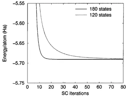
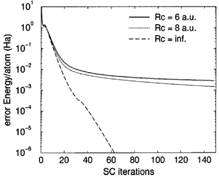
At each step of the iteration process, the computed cor-rections were truncated in order to preserve the confinement of the orbitals in their assigned localization regions. At some point, the truncated part may then become more important than the part actually used. In order to evaluate the accuracy of the localization approximation, it is thus important to compare the Kohn-Sham energies obtained with and without localization for realistic test cases. Figures 3 and 4 show the convergence rates and the absolute error for a 160-atom nanotube. For a fixed number of orbitals, the rate of conver-gence decreases with increasing localization when the num-ber of orbitals is kept fixed. Turning to accuracy, the loga-rithmic plot in Fig. 4 shows that an accuracy of 10⫺2 关Ha/ atom兴for a system of 160 carbon atoms is obtained in 20-35 iterations. Convergence towards more precise results then depends on the localization radii. Significantly more itera-tions are required to reach a precision of 3⫻10⫺3关Ha/atom兴, which is sufficient to obtain a good estimate of eigenvalue differences, e.g., the highest occupied molecular orbital– lowest unoccupied molecular orbital 共HOMO-LUMO兲 gap. The calculated value of this gap depends on the localization radius, see Table II. In particular, Rc⫽8 bohr is sufficient to reproduce the value obtained without the localization ap-proximation.
The accuracy of 3⫻10⫺3 关Ha/atom兴 is not sufficient to
reliably compute total energy differences between different atomic configurations, e.g., in order to extract defect forma-tion energies. However, it is still adequate to compute forces and initiate atomic relaxations. Only a small number of SC iterations is required for each ionic configuration in order to have reliable forces that lead the atoms to their equilibrium positions. The wave-function components that require nu-merous iterations before being completely relaxed are thus improved step by step during the relaxations, and are suffi-ciently well converged by the time the atoms reach their equilibrium positions.
Our tests of relaxation and of total energy differences used the 共10,0兲carbon nanotube, either perfectly symmetric or with the 共5-7-7-5兲 defect.58 The supercell contained 160 atoms. All atoms were relaxed with and without localization constraints. An accurate relaxed atomic configuration could be obtained with a localization radius as small as 6 bohr. Moreover, with a localization radius of 8 bohr the absolute total energies of the relaxed supercells, with and without the defect, were shifted upwards by less than 0.02 关Ha兴. The defect formation energy, defined as the difference between the two total energies, was 0.13 关Ha兴both without localiza-tion and with Rc⫽8 bohr.
A contour plot of a typical localized orbital for the共10,0兲 nanotube is shown in Fig. 5. The orbital is strongly localized in the region of a carbon-carbon bond and smoothly de-creases to zero when approaching the localization boundary. If the localization radius were reduced, one would mainly cut off the tail of the orbital. However, these tails are important in the evaluation of the total energy and calculations with
FIG. 3. Convergence rate for different localization radii for the
共10,0兲carbon nanotube. The supercell contained 160 atoms and the calculations used three orbitals per atom.
FIG. 4. The error, i.e., the difference between the converged DFT total energy without localization and the current energy as a function of the number of self-consistent iterations. Different local-ization radii are compared. The supercell for the 共10,0兲 carbon nanotube contained 160 atoms.
TABLE II. HOMO-LUMO gap for a共10,0兲 nanotube. The
su-percell contained 160 atoms.
共eV兲 Rc⫽5 bohr Rc⫽6 bohr Rc⫽8 bohr Rc⫽⬁
LUMO 1.53 1.27 1.17 1.17
HOMO 0.64 0.41 0.32 0.32
Rc⬍5 bohr may lead to unphysical results.
The computer time for the relaxation of the nonorthogonal orbitals scales as ⬃N(Rc/h)3, where Rc is the localization radius and h the grid spacing. In self-consistent iterations, additional time is spent in N⫻N matrix operations, including
the solution of Eq.共7兲. In Table III, we provide timings for the共5,5兲nanotube with Rc⫽6.2 bohr. Comparisons are made with a constant number of atoms per processor. With a per-fect coding and linear scaling, the timings would be identical for all the examples. The solution of Eq.共7兲, the only strictly
O(N3) part, takes less than 20% of the total time for systems with as many as 3360 orbitals. It is also clear that further restructuring and optimization of the code could result in a significant speedup.
One should stress that the localization of the nonorthogo-nal orbitals reduces the cost of the calculations only for sys-tems significantly larger than the sizes of the individual lo-calization regions. Furthermore, the minimal number of atoms for which nonorthogonal localized orbitals become ad-vantageous depends on the number of nonzero overlaps be-tween the orbitals, and thus on the atomic geometry.
V. SUMMARY AND CONCLUSIONS
An efficient and accurate method for self-consistent ab
initio electronic structure calculations was developed and
implemented on the massively parallel Cray T3E supercom-puter. The method is based on a description of the subspace spanned by the occupied orbitals in a nonorthogonal basis of variationally optimized localized functions. These functions are defined on a grid and are strictly zero outside of spheres centered on the atoms. The localization is essential to achieve a linear scaling of the computational effort for the most expensive part of the calculation—the relaxation of the basis functions and the evaluation of the electronic density. A Mehrstellen finite-difference scheme is used to discretize the Laplacian operator on the grid. A multigrid precondi-tioner has been developed in order to have a very efficient minimization scheme for basis-invariant steepest descent di-rections. Since it appears to be essential for a high conver-gence rate to include unoccupied orbitals in the calculations, a density-matrix formalism is used to define the occupation of the orbitals in the subspace defined by the nonorthogonal basis functions. This requires operations on N⫻N matrices
that scale as O(N3), but when efficiently parallelized this part is relatively cheap when compared to the cost of the relaxation of the orbitals. Our tests show that the O(N3) part is less than 20% of the total time for carbon nanotubes with as many as 1120 atoms.
The accuracy of the calculations can be systematically improved by mesh refinement and/or by extending the local-ization regions of the grid-based orbitals. Numerical tests on carbon nanotubes show that accurate relaxed atomic configu-rations, band-gap, and total energy differences can be ob-tained for localization radii as small as 8 bohr.
ACKNOWLEDGMENTS
We wish to thank Dr. E. L. Briggs for discussions and providing his parallel orthogonal-orbital multigrid code for the Cray T3E. J.-L. F. gratefully acknowledges the financial support of the Fonds National Suisse de la Recherche Scien-tifique. This work was also supported in part by NSF and ONR. Supercomputer calculations were carried out at DoD and NC Supercomputing Centers.
APPENDIX: MATRIX EXPRESSIONS IN A NONORTHOGONAL BASIS
The relation共5兲can be used to derive matrix expressions in the basis⌽. In the basis of the Ritz functions⌿one has at convergence
共B(⌿)兲⫺1H(⌿)⫽⌳,
where⌳is a real diagonal matrix. Therefore,
⌳⫽共CTB(⌽)C兲⫺1共CTH(⌽)C兲
⫽C⫺1共B(⌽)兲⫺1H(⌽)C ⫽CTS关共B(⌽)兲⫺1H(⌽)兴C.
The matrix C is then a solution of the generalized eigenvalue problem
FIG. 5. Contour plot of the square of a typical localized orbital in the plane defined by the cylindrical surface of the共10,0兲 nano-tube. The contour of lowest value共close to zero兲shows the local-ization region with a radius of 6 bohr.
TABLE III. Timing for 1 SC step for electronic structure calcu-lations for共5,5兲nanotubes of several lengths on the Cray T3E. For 140 atoms, the global grid is 96⫻56⫻56. The number of storage functions denotes how many global arrays—extended over the whole grid—were required to store all the localized orbitals.
No. of atoms 140 280 560 1120
No. of orbitals 420 840 1680 3360
No. of PEs 32 64 128 256
No. of storage func. 237 252 255 255
CPU time/PE共s兲 69 82 104 173
HBC⫽SC⌳
for HB⫽S(B(⌽))⫺1H(⌽). Since (B(⌿))⫺1H(⌿) is symmetric at convergence and
HB⫽S共B(⌽)兲⫺1H(⌽)
⫽SC共B(⌿)兲⫺1H(⌿)C⫺1
⫽C⫺T共B(⌿)兲⫺1H(⌿)C⫺1,
HB is also symmetric at convergence. Furthermore,
共B(⌿)兲⫺1H(⌿)⫺I⫽C⫺1关共B(⌽)兲⫺1H(⌽)⫺I兴C.
Using the invariance of the trace of an operator when chang-ing the basis,
⍀关X¯(⌽)兴⫽Tr关共3X¯(⌽)SX¯(⌽)⫺2X¯(⌽)SX¯(⌽)SX¯(⌽)兲
⫻共HB⫺S兲兴
follows then directly from definition共18兲.
*Present address: CASC, Lawrence Livermore National Labora-tory, L-551, Livermore, CA 94551.
1P. Hohenberg and W. Kohn, Phys. Rev. B 136, 864共1964兲.
2W. Kohn and L. J. Sham, Phys. Rev. A 140, 1133共1965兲.
3A. Brandt, Math. Comput. 31, 333共1977兲.
4B. Hermansson and D. Yevick, Phys. Rev. B 33, 7241共1986兲.
5S. R. White, J. W. Wilkins, and M. P. Teter, Phys. Rev. B 39,
5819共1989兲.
6H. Murakami, V. Sonnad, and E. Clementi, Int. J. Quantum
Chem. 42, 785共1992兲.
7E. Tsuchida and M. Tsukada, Phys. Rev. B 52, 5573共1995兲.
8J. E. Pask, B. M. Klein, C. Y. Fong, and P. A. Sterne, Phys. Rev.
B 59, 12 352共1999兲.
9J. Bernholc, J.-Y. Yi, and D. J. Sullivan, Faraday Discuss. Chem.
Soc. 92, 217共1991兲.
10J. R. Chelikowsky, N. Trouiller, and Y. Saad, Phys. Rev. Lett. 72,
1240 共1994兲; J. R. Chelikowsky, N. Trouiller, K. Wu, and Y. Saad, Phys. Rev. B 50, 11 355共1994兲.
11F. Gygi and G. Galli, Phys. Rev. B 52, R2229共1995兲.
12E. L. Briggs, D. J. Sullivan, and J. Bernholc, Phys. Rev. B 52,
R5471共1995兲; 54, 14 362共1996兲.
13A. P. Seitsonen, M. J. Puska, and R. M. Nieminen, Phys. Rev. B
51, 14 057共1995兲.
14J.-L. Fattebert, BIT 36, 509 共1996兲; J. Comput. Phys. 149, 75
共1999兲.
15N. A. Modine, G. Zumbach, and E. Kaxiras, Phys. Rev. B 55,
1337共1997兲.
16T. L. Beck, K. A. Iver, and M. P. Merrick, Int. J. Quantum Chem.
61, 341共1997兲; T. L. Beck, ibid. 65, 477共1997兲.
17F. Ancilotto, P. Blandin, and F. Toigo, Phys. Rev. B 59, 7868
共1999兲.
18K. Cho, T. Arias, J. Joannospoulos, and P. Lam, Phys. Rev. Lett.
71, 1808共1993兲.
19
S. Wei and M. Y. Chou, Phys. Rev. Lett. 76, 2650共1996兲.
20C. J. Tymczak and X.-Q. Wang, Phys. Rev. Lett. 78, 3654共1997兲.
21G. Galli and M. Parrinello, Phys. Rev. Lett. 69, 3547共1992兲.
22L.-W. Wang and M. P. Teter, Phys. Rev. B 46, R12 798共1992兲.
23W. Kohn, Chem. Phys. Lett. 208, 167共1993兲.
24F. Mauri, G. Galli, and R. Car, Phys. Rev. B 47, R9973共1993兲; F.
Mauri and G. Galli, ibid. 50, 4316共1994兲.
25P. Ordejon, D. A. Drabold, M. P. Grumbach, and R. M. Martin,
Phys. Rev. B 48, 14 646共1993兲; P. Ordejon, D. A. Drabold, R. M. Martin, and M. P. Grumbach, ibid. 51, 1456共1995兲.
26E. B. Stechel, A. R. Williams, and P. J. Feibelman, Phys. Rev. B
49, 10 088共1994兲.
27J. Kim, F. Mauri, and G. Galli, Phys. Rev. B 52, 1640共1995兲.
28X.-P. Li, R. W. Nunes, and D. Vanderbilt, Phys. Rev. B 47,
10 891共1993兲.
29M. S. Daw, Phys. Rev. B 47, 10 895共1993兲.
30
R. W. Nunes and D. Vanderbilt, Phys. Rev. B 50, 17 611共1994兲.
31S. Goedecker and L. Colombo, Phys. Rev. Lett. 73, 122共1994兲.
32W. Kohn, Phys. Rev. Lett. 76, 3168共1996兲.
33J. M. Millam and G. E. Scuseria, J. Chem. Phys. 506, 5569
共1997兲.
34E. Hernandez and M. J. Gillan, Phys. Rev. B 51, 10 157共1995兲;
E. Hernandez, M. J. Gillan, and C. M. Goringe, ibid. 53, 7147 共1996兲.
35T. Hoshi and T. Fujiwara, J. Phys. Soc. Jpn. 66, 3710共1997兲.
36W. Yang, Phys. Rev. B 56, 9294共1997兲.
37W. Yang, Phys. Rev. Lett. 66, 1438共1991兲.
38W. Yang and T.-S. Lee, J. Chem. Phys. 103, 5674共1995兲.
39R. Baer and M. Head-Gordon, J. Chem. Phys. 109, 10 159共1998兲.
40S. Baroni and P. Giannozzi, Europhys. Lett. 17, 547共1991兲.
41D. Sanchez-Portal, P. Ordejon, E. Artacho, and J. M. Soler, Int. J.
Quantum Chem. 65, 453共1997兲.
42G. Galli, Curr. Opin. Solid State Mater. Sci. 1, 864共1996兲.
43S. Goedecker, Rev. Mod. Phys. 71, 1085共1999兲.
44L. Collatz, The Numerical Treatment of Differential Equations
共Springer, Berlin, 1966兲.
45M. Buongiorno Nardelli, Phys. Rev. B 60, 7828共1999兲.
46M. Buongiorno Nardelli, J.-L. Fattebert, and J. Bernholc共
unpub-lished兲.
47I. Stich, R. Car, M. Parrinello, and S. Baroni, Phys. Rev. B 39,
4997共1989兲.
48M. P. Teter, M. C. Payne, and D. C. Allan, Phys. Rev. B 40,
12 255共1989兲.
49S. Costiner and S. Taasan, Phys. Rev. E 52, 1181共1995兲.
50D. R. Bowler and M. J. Gillan, Comput. Phys. Commun. 112, 103
共1998兲.
51J. H. Bramble, J. E. Pasciak, and J. Xu, Math. Comput. 55, 1
共1990兲.
52N. Marzari, D. Vanderbilt, and M. C. Payne, Phys. Rev. Lett. 79,
10 289共1997兲.
53C. A. White, P. Maslen, M. S. Lee, and M. Head-Gordon, Chem.
Phys. Lett. 276, 133共1997兲.
54S. Ismael-Beigi and T. A. Arias, Phys. Rev. Lett. 82, 2127共1999兲.
55L. S. Blackford, J. Choi, A. Cleary, E. D’Azevedo, J. Demmel, I.
Dhillon, J. Dongarra, S. Hammarling, G. Henry, A. Petitet, K. Stanley, D. Walker, and R. C. Whaley, SCALAPACK User’s
Guide共SIAM, Philadelphia, 1997兲.
56D. R. Hamann, Phys. Rev. B 40, 2980共1989兲.
57M. Fuchs and M. Scheffler, Comput. Phys. Commun. 119, 67
共1989兲.
58M. Buongiorno Nardelli, B. I. Yakobson, and J. Bernholc, Phys.