Validation and Uncertainty Quantification of a 1x2" NaI Collimated Detector Using Detector Response Functions Created by g03.

ABSTRACT

NELSON, NOEL BENJAMIN. Validation and Uncertainty Quantification of a 1x2" NaI Collimated Detector Using Detector Response Functions Created by g03. (Under the direction of Yousry Azmy.)

© Copyright 2014 by Noel Benjamin Nelson

Validation and Uncertainty Quantification of a 1x2" NaI Collimated Detector Using Detector Response Functions Created by g03

by

Noel Benjamin Nelson

A thesis submitted to the Graduate Faculty of North Carolina State University

in partial fulfillment of the requirements for the Degree of

Master of Science

Nuclear Engineering

Raleigh, North Carolina

2014

APPROVED BY:

Robin Gardner John Mattingly

Ralph Smith Louise Worrall

Yousry Azmy

DEDICATION

BIOGRAPHY

The author was born in a small town in Oregon called John Day, to parents R. Bryan and Deanna Nelson as the youngest of two children. He graduated from Grant Union High School as the Valedic-torian in 2008. He continued his studies at Oregon State University (OSU) for four years in Nuclear Engineering.

At OSU he worked diligently beside his studies as a cook for the university dormitory kitchens and as an undergraduate researcher for the chemistry department. In his chemistry research, he observed the effects of electric voltage, frequency, and amperage on the polymer brush growth of hemoglobin for use in the manufacture of prosthetics. He graduated Summa Cum Laude from Oregon State with an Honors B.S. in nuclear engineering in the summer of 2012.

ACKNOWLEDGEMENTS

Infinite gratitude to my advisor, Dr. Yousry Azmy, for all of his guidance and assistance. All of my committee provided good support and assistance. Dr. Mattingly offered all of his knowledge and expertise in detection. Dr. Gardner and his students Wes Holmes and Adan Calderon were invaluable in learning the g03 software and understanding the intricacies of DRFs. Dr. Smith’s assistance with and class on uncertainty quantification were greatly useful. Without his help I would still have no idea what Bayes theory was let alone how to use it.

TABLE OF CONTENTS

LIST OF TABLES . . . vi

LIST OF FIGURES . . . vii

CHAPTER1 INTRODUCTION . . . 1

1.1 Research Motivation and Goals . . . 1

1.2 Summary of Results and Conclusion . . . 2

CHAPTER2 REVIEW OF THE LITERATURE . . . 4

2.1 NaI Detection and Detector Response . . . 4

2.2 Monte Carlo Based Radiation Transport . . . 10

2.3 Detector Response Functions . . . 12

2.4 Uncertainty Quantification . . . 15

CHAPTER3 EXPERIMENTAL SETUP AND COMPUTATIONAL MODEL . . . 20

3.1 Experimental Setup . . . 20

3.2 Monte Carlo Transport Models . . . 30

CHAPTER4 VALIDATION . . . 34

4.1 Cs-137 Measurement . . . 34

4.2 Co-60 Measurement . . . 37

4.3 Axial HEU Disc Measurement Set . . . 39

4.4 HEU Disc Attenuation Measurement Set . . . 46

CHAPTER5 UNCERTAINTY QUANTIFICATION . . . 48

5.1 Monte Carlo Based Uncertainties . . . 48

5.2 Parameter Uncertainties . . . 53

CHAPTER6 CONCLUSION AND FUTURE WORK . . . 62

6.1 Conclusion . . . 62

6.2 Future Work . . . 64

REFERENCES . . . 65

APPENDIXA ALTERNATIVE METHODS AND MODELS . . . 70

A.1 HEU Disc Response: Separate Versus Combined Peaks . . . 70

A.2 Freqentist and Bayesian Power Law Uncertainty . . . 71

LIST OF TABLES

Table 3.1 Dimensions and activities of calibration sources used for experimental

measure-ments . . . 23

Table 3.2 Gamma ray energies and relative intensities of all sources measured were taken from Brookhaven National Laboratory’s Nudat2.6 database.[28]Unlisted un-certainties were assumed to be one in the last digit. . . 24

Table 3.3 Enrichment of the uranium disc source . . . 27

Table 3.4 Stainless steel alloy composition used in the MCNP simulations. . . 29

Table 4.1 Various photon cross sections (c m2_{/g) from 60 keV to 2 MeV.[25] . . . 39}

Table 5.1 Channel means and associated standard deviations (STD) of the Gaussian fits for the energy calibration. . . 53

Table 5.2 Energy calibration parameter means and standard deviations. . . 54

Table 5.3 Channel means and associated standard deviations of the Gaussian fits for the power law. . . 55

Table 5.4 Linear correlation coefficients for the 81 keV Ba-133 linear Gaussian model fit. . . . 56

Table 5.5 Power law parameter means and standard deviations. . . 57

Table 5.6 Computed spectrum channel means and associated standard deviations of the Gaussian fits for the energy energy shift. . . 58

Table 5.7 Experimental net spectrum channel means and associated standard deviations of the Gaussian fits for the energy shift. . . 59

LIST OF FIGURES

Figure 2.1 A basic NaI detector schematic.[14] . . . 6 Figure 2.2 Predicted detector response spectrum of a medium sized detector with labeled

regions of interest[15]. . . 7 Figure 3.1 A schematic detailing the 1x2" NaI detector used at ORNL. . . 22 Figure 3.2 Photograph of the HEU disc off-axis experiment 41 cm from the detector and 15

cm to the right (x=+15cm). . . 25 Figure 3.3 Dimensions of the HEU disc as prescribed from ORNL. The disc is made of

stainless steel (shell), epoxy (adhesive), and HEU (4.76x0.07cm active source area). . . 26 Figure 3.4 Photograph of the HEU disc attenuation experiment with two stainless steel

plates attached to the detector (11 cm from the source). . . 28 Figure 4.1 Measured and normalized computed responses for the Cs-137 calibration source

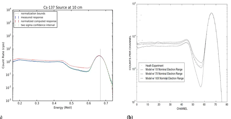
at 10 cm (normalized across bounds) with aluminum can (a) and without aluminum can and collimator (b). . . 34 Figure 4.2 (a) Measured and normalized computed responses for the Cs-137 calibration

source at 10 cm (normalized to the peak). (b) 3x3" NaI detector computed re-sponses over a varying electron range multiplier compared with the measured response from the Heath benchmark. . . 36 Figure 4.3 (a) Measured and normalized computed responses for the Co-60 calibration

source on the detector face using normalization across a range of channels (a) and normalized to the highest intensity peak (b). . . 37 Figure 4.4 Measured and normalized computed responses for the HEU disc at the central

position. . . 38 Figure 4.5 Measured and normalized computed responses for the HEU disc source at y=41

cm and (a) five centimeters left of center x=-5 cm and (b) five centimeters right of center x=5 cm. . . 41 Figure 4.6 Measured and normalized computed responses for the HEU disc source at y=41

cm and (a) ten centimeters left of center x=-10 cm, (b) ten centimeters right of center x=10 cm, (c) fifteen centimeters left of center x=-15 cm, and (d) fifteen centimeters right of center x=15 cm. . . 42 Figure 4.7 Measured and normalized computed responses for the HEU disc source at y=41

cm and (a) twenty centimeters left of center x=-20 cm and (b) twenty cen-timeters right of center x=20 cm. . . 44 Figure 4.8 Measured and normalized computed responses for the HEU disc source with (a)

Figure 5.1 Diagram of the detector to source geometry and the solid angle chosen for the initial source distribution forcing pdf. . . 49 Figure 5.2 MCNP computed fluence and two sigma confidence interval . . . 50 Figure 5.3 HEU disc at 41 cm with DRF densities for the 105 keV peak at channel 33 and the

two sigma confidence interval . . . 51 Figure 5.4 Absolute efficiency of the HEU disc at 41 and two standard deviation confidence

interval . . . 52 Figure A.1 Full simulation of seven peaks vs. six peaks with two combined at 150 keV. . . 70 Figure A.2 Peak normalized computed responses from MCNP with and without the

CHAPTER

1

INTRODUCTION

1.1

Research Motivation and Goals

Detector response functions (DRF) have become an area of increasing scientific interest for the last thirty years in several industrial detection applications. These applications include coal spectrometry for composition and location in the interest of mining, oil-well logging, radio-tracing in medicine, computerized tomography (CT) scans, and holdup source characterization. DRF uses could be extended to nuclear safeguards and security applications as well such as border monitoring for illegal transport of radioactive materials, cargo and package monitoring, and unknown source identification at source recovery sites. However, a rigorous mathematical formulation of the DRF has yet to be developed. Therefore, a few working empirical and stochastic approaches have been developed instead to create DRFs.

1.2. SUMMARY OF RESULTS AND CONCLUSION CHAPTER 1. INTRODUCTION

Much of the most recent work on DRFs has been performed by Dr. Robin Gardner and his research group at North Carolina State University. Gardner has developed a fairly accurate DRF model through empirical curve fitting and Monte Carlo analysis. The DRF has been validated against experimental measurements taken by Heath and was found to agree within two standard deviations of the experimental results from Heath. The measurements were taken with 3x3" and 6x6" NaI detectors and Cs-137 sources centered on the detector’s front axis at a distance of 10 cm. There was agreement with the Heath benchmark detector measurements of the same sizes up to two standard deviations of the measured Poisson error.[16][4]

Some validation work has been carried out on the source positioned off-axis relative to the detector and with intervening material placed between the source and detector pair. This was done in the interest of developing spectrum analysis software specific to the Compton continuum in order to identify attenuators and account for off-axis geometries. The software that accomplishes this purpose is still under development, but once it reaches fruition it should be considered for incorporation into future works that employ DRFs.

The goal of this work was to use the NaI DRF model developed by Gardner to characterize a NaI 1x2" detector for on-axis geometries, off-axis geometries and attenuated configurations and to validate it against experimental measurements. Also, uncertainty in the model was calculated by Frequentist and Bayesian methods, and compared to measurement and Monte Carlo transport uncertainties. The overarching goal is to incorporate an accurate DRF model into an holdup problem approach to the holdup application to characterize special nuclear material (SNM) deposits at nuclear production and processing facilities.

1.2

Summary of Results and Conclusion

There were three major sets of measurements: on-axis detection of calibration sources, off-axis measurements with a highly enriched uranium (HEU) disc, and the HEU disc with steel plate attenuation between the source and detector. In terms of the calibration source spectra with one or two peaks and a Compton continuum, the computed spectrum predicted the peak well within two standard deviations of the experimental count rate, but overestimated the continuum and valley between the peak and Compton edge. This problem likely came from miscalibration of the electron range multiplier (Equation 2.4) used originally for an uncollimated 3x3" detector, as the same effect was observed in Gardner’s original validation work when the multiplier was set too low.

1.2. SUMMARY OF RESULTS AND CONCLUSION CHAPTER 1. INTRODUCTION

two standard deviations of the measured count rate, but underestimated the convolved peak at (150 keV) and did not reproduce the lead backscatter peak near 100 keV. This was due to scattering with the lead collimator that was unaccounted for by the DRF model, as the model currently only reproduces the effects of scattering within the detector crystal.

Finally, uncertainty quantification of the model took place on every calculated quantity from the flux calculation in MCNP to the Gaussian peak fits for shifting the program. Where the uncertainty was controllable by the number of particle histories chosen in Monte Carlo simulations, it was reduced below the lowest measured uncertainty. Where it was constrained to the accuracy of the model for least squares fitting, the reduced chi-square test was performed to check for goodness of fit.

CHAPTER

2

REVIEW OF THE LITERATURE

The purpose of this literature review is to lay the foundation for the development of the sodium iodide (NaI) detector response function and the corresponding uncertainty quantification based on the results and discoveries of previous scientists in the field of gamma radiation transport and detection. First, the history and development of the NaI detector and its supplementary equipment will be summarized. Then the major developments in Monte Carlo based transport theory relevant to the construction of DRFs will be discussed. The third section will detail the creation of detector response models. Finally, the last section will concern relevant Bayesian uncertainty quantification methods.

2.1

NaI Detection and Detector Response

Before detector response functions were even considered, detector responses and operation prin-ciples had to be developed. The detector of interest in our work is a sodium iodide scintillation detector. Scintillation is simply the emission of a visible photon from a material by dexcitation of an electron following its interaction with incident gamma. The favorable scintillation properties of NaI doped with trace amounts of Thallium (NaI(Tl))were first discovered by Robert Hofstadter in 1948

2.1. NAI DETECTION AND DETECTOR RESPONSE CHAPTER 2. REV. OF THE LIT.

Hofstadter concluded that NaI(Tl) would be an efficent detector of ionizing radiation. He deter-mined this based off of the duration of light emission, distribution of light pulses, particle energy discrimination (therefore radioactive source discrimination), and the proportionality of counting events to voltage and amplifier gain. He compared some of these characteristics with another detec-tion material, anthracene, while merely verifying other materials to conclude that NaI(Tl) is a viable detector.

A NaI(Tl) crystal alone does not make a detector. Light emitted from the crystal after an interac-tion is captured via a photoelectric effect interacinterac-tion with the photocathode of the detector. The freed electrons are multiplied and amplified into a detectable electronic signal pulse by the photo-multiplier tube (PMT). The first photphoto-multiplier tube was developed by Harley Iams and Bernard Salzberg much earlier than Hofstadter, in 1935.[6]

They observed the amplification of the primary photocurrent (a stream of electrons) through the effects of secondary emission and the photoelectric effect. Secondary emission is when an electron current strikes a charged plate and releases more electrons than were absorbed by the plate. Iams and Salzberg found that their photomultiplier tube was superior to gas phototubes as they had no interference at high audio frequencies from small fluctuations in its current supply, while still comparable to the vacuum phototubes (other detector PMT candidates). This model is the basis for modern PMT’s.

The small electronic output signal from the PMT is then amplified and reshaped from a sharp edged pulse into a wider pulse (based on the difference between a rising and falling exponential) for easy processing. This wider pulse is passed to the multichannel analyzer (MCA), which outputs a differential pulse height spectrum (DPHS) also known as a detector response. A DPHS is created simply by setting a small pulse amplitude window to count pulses of varying heights within the window within a counting period between two energies called a channel. An MCA does this for hundreds of channels at once across the entire detector’s energy range. The detector’s energy range is determined partially by size and pulse amplitude gain settings. Low energy photons are resolved better by higher gain and the inverse is true for high energy photons. Also, large detectors have better interaction cross sections with higher energy gammas.

The first MCA was invented by George Kelly at Oak Ridge National Laboratories (ORNL) in 1953. Kelly prized his method as being much faster than older methods using single channel analyzers and more reliable with channel width and position errors meeting statistical standards set at the time.

[7]Since then MCAs and pulse processing equipment have become more efficient and compact, such that they are often combined together into one machine that is controlled by local desktop software.

2.1. NAI DETECTION AND DETECTOR RESPONSE CHAPTER 2. REV. OF THE LIT.

of the detection process and pulse processing equipment, please refer to KNOLL’s book on Radiation Detection and Measurement.

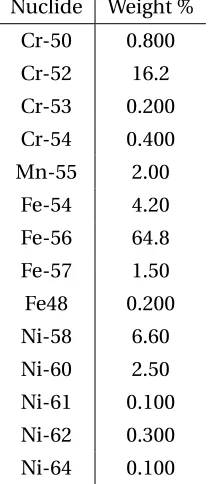
Figure 2.1A basic NaI detector schematic.[14]

In most cases, the current pulse is sent to the pulse processing equipment and MCA to convert the small collection of electrons from the PMT into a response spectrum. Detector response spectra can be used to locate and identify sources of gamma radiation since the response peak channel is proportional to the incident energy of the incident radiation. It is proportional because the relationship between the energy deposited by radiation in the NaI crystal to the scintillation light yield is fairly linear for energies above 100 keV. A quadratic energy calibration using at least three known sources can account for the slight nonproportionality of detector channel to energy, and thereby be used to identify the energy of the incident radiation from other unknown sources.

2.1. NAI DETECTION AND DETECTOR RESPONSE CHAPTER 2. REV. OF THE LIT.

Figure 2.2Predicted detector response spectrum of a medium sized detector with labeled regions of inter-est[15]

Every section of the response spectrum is the result of a combination of one or more photon interactions with the detector crystal or its casing material. The three major types of photon in-teractions with matter include: photoelectric effect, Compton scatter, and pair production. The photoelectric effect occurs when a photon is absorbed by an atom, and a bound electron is then expelled from that atom. Compton scatter occurs when a photon is merely deflected by an atom, and thereby loses a fraction of its energy and changes direction. The third interaction occurs when a high energy photon (greater than 1.022 MeV) interacts with the nuclear electromagnetic field and creates an electron-positron pair that are propelled in opposing directions. Further details of basic particle interactions can be found in Hubbell’s report on Photon Cross Sections.[5]

Knoll’s book mentions several spectral components that appear in a typical response spectrum as a result of the three basic particle interactions. These include the full energy peak, Compton continuum, and the several other types of peaks that appear in Figure 2.2.

2.1. NAI DETECTION AND DETECTOR RESPONSE CHAPTER 2. REV. OF THE LIT.

increasing incident particle energy. For most measurements it varies from 8-15%.[17]

The continuum is created by the probable set of energy depositions from Compton scatter at various angles of deflection with incomplete energy deposition in the detector crystal. The continuum can also be affected by Compton scattering outside of the detector where the deflected photon is detected instead of the electron that is freed when the scatter occurs in the detector crystal. One example is a backscatter peak where the photon scatters at a 180o angle from the rear detector wall into the detector crystal.[9]The shape of the continuum and backscatter peaks can also be significantly affected if an attenuator is in placed front of the source, or if the source is off-axis affecting the number of photons that scatter off of the detector casing into the crystal at a given energy. It is useful in many applications to be able to match different continuum shapes to their most probable cause.

Escape peaks arise when pair production occurs in the detector crystal, but one (single) or both (double) the photons that are created from the annihilation of the resulting positron escape. These events typically occur in small detectors near the edge of the crystal where it is easy for electrons to escape the crystal. When the positron-electron pair is created, the original photon loses the amount of energy required to create the mass of an electron and a positron. The rest mass of both an electron and a positron are approximately 511 keV. The electron created will not contribute much to the response, but the positron does once it annihilates with another electron. The annihilation event creates two photons equivalent to the lost rest mass of each particle, 511 keV, which travel in opposite directions. If both photons escape frequently without depositing energy in the detector crystal, then a double escape will appear in the spectrum at the energy of the incident gamma minus two times the electron rest mass (Eo−1.022M e V). If only one of the photons deposit their energy in

the crystal frequently, then a single escape peak will appear in the spectrum at the original incident gamma energy minus one electron rest mass (Eo−0.511M e V).

An annihilation peak is observed when pair production occurs in the detector shielding, or alternatively in the source shielding, and one of the 0.511 MeV photons created in the following positron annihilation event is detected. Finally, characteristic X-rays (usuallyEX−r a y <100k e V) are

created from the de-excitation of atoms that were involved in a photoelectric event with an incident photon. Typically, the emitted X-rays is reabsorbed by the detector medium and contributes to the full energy peak. However, if the detector is fairly small and these X-rays escape, then an X-ray escape peak is observed in the response slightly below the full-energy peak (Eo−EX−r a y).

2.1. NAI DETECTION AND DETECTOR RESPONSE CHAPTER 2. REV. OF THE LIT.

NaI(Tl) detectors are their large decay times between pulses and fairly low energy resolution (wide full-energy peaks).

Decay time simply refers to the amount of time it takes for the ionized electrons from a detection event to decay from an excited state at the Thallium activator sites back to the ground state and produce scintillation photons for the detector pulse. Subsequent incident gamma rays cannot be detected during this decay time. For NaI(Tl), the decay time is 230 ns, which is much slower than an organic scintillator which have typial decay times around 2 ns. Therefore, organic scintillators are preferred for fast counting experiments where spectral information is less important than timing.

Knoll defines Energy resolution asR = F W H M_H

o where F W H M is the full width at half the

maximum of the full energy peak andH_ois the height of the peak at its center. Therefore, a lower resolution means the peak is narrower compared to its height and requires fewer channels to define the peak (better for distinguishing peaks that are close together in energy). Because FWHM is energy dependent and dependent on the statistical fluctuation in a given measurement, for a given detector type the Poisson limit of the resolution is defined asR|P o i s s o n l i m i t=2.35/

p

N, where N is the total number of information carriers. For NaI detectors, the theoretical limit would be about 1.2%, since it produces around N=38,000 information carriers (scintillation photons), whereas a semiconductor detector withN =105−106has a much lower limit of about 2.25%. NaI does not approach this limit closely though, as their is further loss of those scintillation photons from emission to absorption in the photocathode.

However, NaI(Tl) is the best scintillation detector for spectroscopy applications (not fast pulse timing experiments) because it has one of the highest photon absorption to light yield of 38,000 photons/MeV. Only CsI(Tl) and Cs(Na) are higher with 65,000 and 39,000 photons/MeV respectively. Cs(Na) has pretty equivalent properties to NaI, but has a much slower decay time between pulses. Additionally, CsI(Tl) has a bad emission wavelength (540 nm) that doesn’t couple well with standard PMTs absorption spectrum (400-450 nm). Due to these weaknesses, generally NaI(Tl) is preferred among scintillators.[9]

For fine measurement applications in the lab, however, a semiconductor detector made of high purity Germanium (HPGe) is usually preferred. It has better resolution overall ranging from 0.13-1%.

2.2. MONTE CARLO BASED RADIATION TRANSPORT CHAPTER 2. REV. OF THE LIT.

2.2

Monte Carlo Based Radiation Transport

Detector responses can be predicted mathematically by taking the product of the detector’s response function (DRF) with the flux (particle speed per volume) of the radiation incident on the detector

[9]. The particle flux can be predicted from the solution of the Boltzmann transport equation at the location of the detector crystal due to a given source. The equation was first derived by Ludwig Boltzmann in 1872.[8]Since then, many approximate methods have been developed for solving the Boltzmann equation under certain assumptions suitable for a variety of applications.

One of the more popular transport methods is the Monte Carlo method. The Monte Carlo method does not solve the transport equation itself, instead it simulates the particles and their trajectories through the modeled materials using sequences of pseudo-random numbers. Then it determines the average state of the physical system from the average behavior of the particles.[13] The software chosen for these calculations is the Monte Carlo Neutron-Particle (MCNP) transport code. It was created formally in 1977, though its roots extend back to the late 1940s, at the dawn of the nuclear age. This section outlines the basics of MC transport for calculating incident flux on the detector for the purpose of validating the DRF.

First, particles are simulated and transported according to Boltzmann physics within the volume of interest. Instead of solving the transport explicitly for the entire volume to obtain the flux, the fluence is calculated inside the detector volume only. The fluence,Φ, is defined as

Φ= lim

∆V→0[

P

isi

∆V ]. (2.1)

If a large number of particles were simulated, this quantity could be calculated directly.[10] Simply by tracking particles through a cell of interest and summing up all of the particle tracks within the very small discrete spheres, the flux is approximated. For large volumes like nuclear power reactors this method becomes inefficient and less accurate. For small detector volumes, however, it works quite well.[2]

That is how Monte Carlo simulation works by simulating moving particles directly and tracking them through simulated media. Particle tracks from birth in a source to death (absorption or escape) from the system including all intervening scatters are called histories. The number of particle histories (N) executed in an MCNP run is chosen in order to obtain the desired level of uncertainty in the calculated quantities.

2.2. MONTE CARLO BASED RADIATION TRANSPORT CHAPTER 2. REV. OF THE LIT.

distributions called cross sections. A photon microscopic cross section,σr e a c t i o n t y p e is defined

as the probability of a photon-nuclear reaction with a nucleus.[1]It can also be thought of as the effective cross sectional area presented by the nucleus to the beam of incident photons, and cross sections have units ofc m2. Cross sections depend on energy, material, and interaction type.

Often microscopic cross sections are multiplied by the atom density of the medium to make a macroscopic cross section. Photon macroscopic cross sections,µi n t e r a c t i o n, (also called attenuation

coefficients) are simply the probability of a certain interaction with the medium occurring per unit path length traveled.[1]Summing the macroscopic cross sections of every interaction type yields the total attenuation cross section,µ. There are several minor interaction cross sections (Raleigh scattering, Thompson scattering, etc.), but the largest contributions for photons come from the three aforementioned interactions: photoelectric effect, Compton scatter, and pair production.

If these interactions produce secondary particles, they too are stored and tracked as new histories after the original particles terminate. Finally, after each particle history has been recorded, the particle track (si) through the detector volume is added to the running tally calculating the flux

according to the average of Equation (1) piece by piece until all the histories are tallied.

The Monte Carlo transport method is very effective and simple, but can be inefficient and have high variances if variance reduction techniques are not applied. Variance in Monte Carlo is based on the number of histories run, so the simplest way to reduce variance in such a calculation is to run more particle histories. Sometimes this is not feasible (rare events), therefore variance reduction techniques are used instead. In Exploring Monte Carlo Methods by Dunn and Shultis the most common variance techniques are described, which include particle weighting, truncation, splitting, and Russian roulette.

The first method is called weighting. A biased multiplier (called a weight) may be applied to particles undergoing desired physical events in order to force rare interactions to occur more often without running as large numbers of histories. The biased particles’ contribution to the tally (the score) is then renormalized by mulitplying by 1/w e i g h t. This ensures that desired events are well sampled, but the tally still represents an unbiased system.

2.3. DETECTOR RESPONSE FUNCTIONS CHAPTER 2. REV. OF THE LIT.

For implicit absorption, particles are never allowed to be killed by absorption. Instead, every time an absorption event would occur, the particle’s weight is reduced by multiplying its weight by the probability of survival (1−µa

µ ). Then a particle interaction is chosen for the particle from the

remaining non-absorption interaction probabilities. Therefore, in this scenario, a particle may only be killed by leaking out of the system. To prevent buildup of low weight particles in the system, this technique is usually paired with the Russian roulette technique.

Truncation methods set cutoff limits for when a particle should be terminated. For example, if a particle reaches a position outside of the system of interest (leakage), then tracking would be terminated. Other examples, include unfavorable directions, low energies, and low weights unlikely to contribute much to the tally of interest. Truncation helps to kill particles early that are only wasting computational resources.

Finally, splitting and Russian roulette schemes are almost always applied together. Splitting occurs when a particle enters a region designated of higher importance and interest (e.g. the cell where a tally is calculated, and it is split into m particles. Each particle weight is then given by a 1/m fraction of the weight of the original particle. Russian roulette is exactly the opposite of splitting. Particles that travel into regions of low interest may be killed by random selection. Some 1/m fraction of particles are killed, and the remainder increased in weight by a factor of m.[2]

All of the variance reduction techniques reduce variance without biasing the tallies, if used correctly. Often these techniques increase computational efficiency and decrease computation times. Many production Monte Carlo transport codes apply some of these techniques automatically, while allowing the others to be chosen as options.

In this work, the Los Alamos National Laboratories (LANL) code Monte Carlo Neutron Transport code (MCNP) was used to compute flux tallies incident on the 1x2" NaI detector model. The code was originally implemented for neutron transport, but can also be used for other particle transport, such as photon transport. Monte Carlo based calculation was also used in part to calculate the DRF.

2.3

Detector Response Functions

The DRF (R(E,h)) is defined as the probability that a photon incident on the detector with energy E will give rise to a pulse with heighth.[18]DRFs are useful for converting flux to counting spectra, calculating detector efficiencies, and also for the reverse, transforming responses back into flux. The latter purpose will be explored more in future research, but in this work focus will remain on the former purpose.

2.3. DETECTOR RESPONSE FUNCTIONS CHAPTER 2. REV. OF THE LIT.

Monte Carlo simulation. Gardner’s original work with his colleague Avneet Sood validated 3x3 NaI synthetic detector responses to the Heath benchmark Cs-137 spectrum. Gardner’s model was found to be more efficient (required far less particle histories for accurate calculation) and was shown to match better with the Heath experiments than MCNP’s F8 response tally.[16]It was chosen for our work for these reasons and also because MCNP simulates responses according to direct energy deposition in the detector crystal. It generates no DRF, and a DRF will be needed for future holdup work.

The Heath experiments were performed on a 3x3" NaI detector in 1964 as a benchmark for a number of gamma sources. All measurements were very high fidelity. The measurements were performed in a lead shielded box to reduce background radiation and all spectra were counted well over 10,000 counts in the peak channel for less than 1% counting uncertainty. For further information, see Heath’s Gamma Ray Spectrum Catalogue.[4]

Gardner’s model generates a DRF for a desired detector size, source distance, and source energy (single peak), through the following set of steps. First, Gardner’s model takes into account the non-linear dependence of NaI scintillation efficiency (s c i n t i l l a t i o n l i g h t y i e l d_{e n e r g y d e p o s i t e d} ) on the energy deposited in the detector by the incident photon. As mentioned before (section 2.1), the nonlinearity in scin-tillation efficiency is an inherent property of NaI(Tl) crystals, and it is particularly pronounced at energies below 100 keV. However, this nonlinearity is still significant for all incident energies below 3 MeV. Gardner used the following nonlinear empirical relationship (from fits to experimental data) to calculate scintillation efficiency for his DRF

S(Ee) =1+k1e x p[−(l n Ee−k2)2/k3],

Ee ≥10k e V,

S(Ee) =1+k1e x p[−(l n Ee−k2)2/k4], (2.2)

Ee ≤10k e V,

whereEe is electron energy in keV.k1is 0.245, andk2isl n10=2.30258.k3is 7.1635, andk4is

5.1946. The electrons are the very same electrons that are involved in interactions with photons incident on the detector crystal. The second step involves Monte Carlo particle transport simulation in which each scattered electron that deposits energy in the detector is multiplied by the scintillation efficiency (Equation 2.2) at the energy deposited.[16]

2.3. DETECTOR RESPONSE FUNCTIONS CHAPTER 2. REV. OF THE LIT.

the spectra. Only about 100,000 particle histories are necessary to produce results with uncertainty under 1%, whereas MCNP F8 Gaussian energy broadened (GEB) spectra require on the order of billions of particles to produce the same precision. The difference typically saves about a day in computation time.

Next, the peaks were stripped from the response spectra so that each contiuum could be pro-cessed alone. Principle component analysis (PCA) was performed on the correlated response vari-ables and the covariance matrix to produce a small set of uncorrelated varivari-ables (principal com-ponents). The principal components and the mean vector were stored as data and can reproduce accurate continuum easily when multiplied with the desired channels vector.Essentially, the contin-uum can be recalled quickly without the need to be regenerated by Monte Carlo simulation for each DRF generated.

So, when a new DRF needs to be generated, the algorithm need only to generate the full-energy peak of interest by Monte Carlo transport simulation and adds this contribution to the continuum to produce the desired DRF.[22]The modified version of Peplow’s code (adjusted by the nonlinear scintillation efficiency) is called g03. The code is in the process of being updated and is proprietary to the Center for Engineering Applications of Radioisotopes (CEAR).

Finally, the Monte Carlo simulation of g03 is modified by several empirical equations to correct pieces of the spectra that are not simulated fully by the Monte Carlo calculation. The g03 DRF peak section is spread according to the following power law (Equation (2.3))

σT(EI) =a EIb, (2.3)

whereaandb are empirical fit parameters, andEI is the energy of the incident gamma ray. This

law is simply an empirical relation that comes from a Least Squares fit of the standard deviations of experimentally measured full-energy peak responses produced by the detector of interest.[16]

2.4. UNCERTAINTY QUANTIFICATION CHAPTER 2. REV. OF THE LIT.

Re=1+A1e x p(−A2EI) +A3e x p(−A4EI) (2.4)

A1=39.662,A2=3.4052,A3=1.5434,A4=0.1576,

whereEI is the energy of the incident photon, andA1−A4are parameters fit from experimental

responses. This factor is a pseudo-electron range equation designed to correct the magnitude of the synthetic Compton continuum produced by the Gardner’s DRF. It was fit through trial and error for 3x3" NaI detectors and may not apply to the detector of interest in this work (1x2" NaI detector).[23] Responses, thus, may be measured or calculated. Validation of Gardner’s model has already been completed on some levels, but almost no uncertainty quantification of the model has been performed. The primary goal of this work is to conduct a validation exercise of the DRF for a specific NaI detector of interest and account for its uncertainties.

2.4

Uncertainty Quantification

In the process of comparing measured to computational model results there are three types of uncertainty in practice. There is measurement uncertainty, model uncertainty, and numerical (simulation) uncertainty. Quantifying uncertainty is important in determining the precision of the model and the computed results. The more precise a result is, the more likely it can be reproduced, and the higher the level of confidence in the applicability of the computational model.

Measurement uncertainty for detection and counting was found to follow a Poisson distribution for a single measurement. This is because the decay of a nucleus is a binary process. It either decays or it does not. The chance of decay per unit time is constant and rather small for a large number of nuclei and a short measurement time (compared to the nuclide’s half-life). A binomial distribution under these conditions (constant and small probability of success) will reduce to a Poisson distribution.[9]

In a Poisson distribution the variance is equal to the mean (the number of counts). Therefore, the variance of the measurement is equal to the mean number of counts. In a single measurement this would be the number of counts measured in a detector channel. The standard deviation is then simply the square root of this count, and the fractional standard deviation (relative to the total count) is one divided by the root of the count.

2.4. UNCERTAINTY QUANTIFICATION CHAPTER 2. REV. OF THE LIT.

independent of one another, then a general formula exists for calculating total uncertainty of the final quantity (Equation 2.5)

σ2

u= (

∂u ∂x)

2_σ2

x+ (

∂u ∂y)

2_σ2

y+ (

∂u ∂z)

2_σ2

z+/l d o t s, (2.5)

whereu =u(x,y,z, . . .)is the quantity derived from basic quantities (x,y,z, . . .)with known variances (σ2_{v a r i a b l e}). The formula is useful for determining the associated uncertainties of many quantities (e.g. count rates and net counts) for various purposes, such as those used in the reduced chi-square test described near the end of this section.[9]

It turns out that simulation uncertainty for Monte Carlo transport calculation is very similar to that of measurement uncertainty. This is due to the fact that the particles themselves are being simulated and tracked as a psuedo-random process. Measurement standard deviation is equivalent to the square root of the number of counts (the mean) in a channel. So it makes sense that the Monte Carlo standard deviation is simply the square root of the number of particle histories in a tally bin. The fractional standard deviation is simply equivalent to the reciprical of the standard deviation.[2]

Determination of the model parameter uncertainty is a more difficult task. For this purpose, there are two major statistical methods to choose from: Bayesian and Frequentist Theory. Since the core of Frequentist Theory requires a large number of data points, a Bayesian method was naturally chosen for the power law Gaussian fits, power law, and the energy calibration fits. Whereas Freqentist methods were chosen for the normal Gaussian fits for shifting spectra and the Gaussian fits of the peaks of experimental spectra for the energy calibration due to the abundance of channels in the peaks of those spectra and for efficient calculation.

Smith’s book, Uncertainty Quantification, describes Frequentist and Bayesian statistics quite well. In both methods, parameter means of each relationship were found via the method of nonlinear least squares. This method solves for the mean parameter values that produced the lowest value of the L₂norm (sum of the squares) of the error. Frequentist methods treat these values as the parameter means and subsequently calculates a Chi squared and covariance matrix to determine the parameter uncertainties. Bayesian methods only use the means for an initial guess (priori information). Further details of least squares methods can typically be found in advanced linear algebra texts. With parameter derivatives and error variance, the Chi squared and covariance matrices can be calculated.

First, however, the error variance must be calculated from the residuals. The error variance is defined as follows

σ2₌ 1

n−pR

T_{R (2.6)}

2.4. UNCERTAINTY QUANTIFICATION CHAPTER 2. REV. OF THE LIT.

by least squares and the experimental data (R=Ye x p e r i m e n t a l−fm o d e l(q)). Also,nis the number of

parameters, andpis the number of model parameters. Next theχmatrix can be calculated as simply the derivative of the model with respect to each parameter,k at each data point i (χi k(q) =∂_∂fiq(kq)).

Using the square of theχmatrix and the error variance the covariance matrix can simply be defined as

V =σ2[χT(q)χ(q)]−1. (2.7) The covariance matrix contains each parameter variance along its diagonal. Simply take the square root of the diagonal values to find the parameter standard deviations. The Frequentist method is very accurate and quick to calculate for cases where there are many more experimental data points than the number of parameters. However, when confidence in a fit is lower due to fewer data points, Bayesian codes fair better.[11]

Bayes theorem expressed in words simply states that parameters are random variables with associated probabilistic densities that make use of known information or new information obtained from conducted measurements. This method picks the best posterior density that reflects the distri-bution of parameter values based on sampled observations. In other words it finds the probability density functions (pdfs) of model parameters that maximizes the likelihood function. Further details of the likelihood function and Bayesian theory are given in Smith’s Book or his reference D. Calvetti and E. Somersalo, Introduction to Bayesian Scientific Computing.

DRAM was used to calculate Bayesian model parameter uncertainties. From Haario’s article "DRAM: Efficient adaptive MCMC" one learns that DRAM stands for Delayed Rejection Adaptive Metropolis algorithm. In this work it is used to estimate the most likely means of the model of interests parameters to verify those determined by least squares fits by employing Monte Carlo random sampling of the parameter values, called chains. DRAM also determines the uncertainty in the parameters from the direct statistical variations in the parameter chains.

2.4. UNCERTAINTY QUANTIFICATION CHAPTER 2. REV. OF THE LIT.

Using regular statistical methods, again the parameter standard deviations can be estimated from the chains of random parameter values.

DRAM works along the same principles, except that the rejection condition is augmented with a more advanced algorithm that increases the probability of acceptance (promoting mixing or broader exploration of the chains). Also, DRAM adapts by suggesting a Gaussian proposal distribution centered at each chain position and retrieves more information about the posterior using it to update the covariance matrix. Together these advancements make a much more efficient algorithm than basic RWM.[19]

Additionally, both Frequentist and Bayesian methods give estimates of the model parameters that best reproduce a curve along the measured data points. Sometimes, least squares fits and maximum likelihood estimates can produce poor curve fits. So, from Bevington and Robinson’s Data Reduction and Error Analysis, one can obtain two useful tools for model examination: the reduced chi-square test and linear correlation coefficients.

The reduced chi-square test helps to provide a quantified measurement of the goodness of fit. The definition of the reduced chi-square is shown by Equation 2.8.

χ2₌

n

X

j=1

[h(x_j)−y(x_j)]2

σj(h)2

χ2

v=χ

2_{/v, (2.8)}

where n is the total number of data points.h(xj)is the measurement, andy(xj)is the model

solution at data point j. Also,σj(h)2is the variance in the measurement at data point j, andv is

the number of degrees of freedom (v=n−p) where p is the number of parameters. In our work, the variance will likely be the poisson variance for a simple count spectrum, or the propagated uncertainty for net counts and count rates. A reduced chi-square test will produce a value equal to one for an ideal case, however, it is generally considered to be still a good fit for values less than ten. Values less than one simply mean that the spectrum was overfit, and may have required a simpler model or fewer data points to produce a similar result.

Furthermore, in the event of a poor fit, the model can be examined more closely by examining the linear correlation coefficients. The linear correlation coefficient matrix can be calculated as follows (Equation 2.9):

ρj k=

σ2

j k

σjσk

(2.9)

2.4. UNCERTAINTY QUANTIFICATION CHAPTER 2. REV. OF THE LIT.

are the diagonal standard deviations of the parameters from the covariance matrix (σj j andσk k).

CHAPTER

3

EXPERIMENTAL SETUP AND

COMPUTATIONAL MODEL

This section will detail the experimental setup and the Monte Carlo computational transport models used to simulate the experiment’s geometric configuration and calculate the flux incident on the detector. A detector description will also be provided, as well as how the detector intrinsic efficiency was calculated. The Monte Carlo calculated quantities are necessary for calculating response spectra for comparison against those obtained via experimental measurements with the actual detector.

3.1

Experimental Setup

The entire experimental campaign was designed and performed at the Safeguards Laboratory at Oak Ridge National Laboratory. The initial campaign was completed over the course of a couple of weeks in June of 2013. Further measurements (such as those for the power law fit) were taken on various days over the course of the spring of 2014, courtesy of ORNL personnel. All sources and detection equipment were provided by ORNL. Each measurement was taken with the same detector, detection equipment, and settings.

3.1. EXPERIMENTAL SETUP CHAPTER 3. EXP. SETUP AND COMP. MODEL

1 12 11 5.078 4.782 3.100 2.540 2.254 0.948

4.288 1.430

6.571 5.080 1.044 2.771 0.320 E E F SECTION E-E

4 7 6 8

10 5 2 3 9 0.048 DETAIL F SCALE 2 : 1

ITEM

NO. PART Material

1 Case Aluminum

2 Plug Aluminum

3 Electronic Housing Void

4 Rear Shield Lead

5 Polymer plate Plastic

6 Steel Enclosure Stainless Steel

7 PMT Void

8 Crystal NaI

9 Tin Shield Tin

10 Collimator Lead

11 Collimator Front Lead

12 Front Cap Aluminum

ORNL 1x2" NaI Detector

DO NOT SCALE DRAWING

NAIDET

SHEET 1 OF 1

8/22/14 NBN

UNLESS OTHERWISE SPECIFIED:

SCALE: 1:2.5WEIGHT:

REV DWG. NO.

A

DIMENSIONS ARE IN CENTIMETERS TOLERANCES: 0.001 FRACTIONAL ANGULAR: MACH BEND TWO PLACE DECIMAL THREE PLACE DECIMAL

5 4 3 2 1

3.1. EXPERIMENTAL SETUP CHAPTER 3. EXP. SETUP AND COMP. MODEL

As can be seen, the detector is well shielded with lead except on the front face where the col-limator aperture allows radiation into the detector from a limited extent of directions covering the corresponding fraction of the unit sphere. Hence, the detector has approximately a 45 degree in-axial-plane angle of vision from the center of its circular front. Contributions to the detector response from any source of radiation far enough off of the axis of the cylindrical detector will be significantly attenuated and radiation incident on the side or rear of the detector will not likely contribute to the measured response spectrum (except for very high energy photons that are not suf-ficiently attenuated by the detector’s lead collimator). The rest of the detector components are fairly standard. It has a PMT, an aluminum sheath (container), etc., as shown in the detector schematic, Fig. 3.1.

Overall, measurements were taken far away from the walls on a table with at most a aluminum tee in the setup. Scattering off of the plastic table, walls, and floor were very unlikely since there is a high probability for interaction of gamma-ray photons with high Z materials. The tee included a small scattering possibility, but it was considered negligible. Therefore, the room geometry and the aluminum tee were not simulated. Only the source, detector, and the air in between were simulated.

In the first set of experiments, a source was placed at a set distance from the detector center (on-axis). The source was held in place on a ring stand, or taped to the front of the detector (for quick counts). The source was typically a button calibration source with known activity and dimensions. These measurements were performed for base validation, energy calibration of the detector, and power law fitting for the DRF.

The parameters of all of the calibration sources used for validation are listed in Table 3.1. Details of the sources used for the energy calibration and the power law fit are not reported here, as these measurements were only intended for determining detector properties.

Table 3.1Dimensions and activities of calibration sources used for experimental measurements

Source A.R. (cm) Thick. (cm) Act. (µC i) Created Measured Act. Meas. (µC i) Cs-137 0.25 0.318 5.01 9/28/2005 2/20/2014 4.13±0.62

Co-60 0.25 0.318 0.8516 3/1/2002 6/21/2013 0.1927±0.029

Note: All calibration sources used in this work were created by Eckert and Ziegler, and the active source dimensions (active radius, A.R., and thickness) used in the MCNP model were taken from the Type D disc model in the catalog. Furthermore, according to the supplier "Sources are manufactured with contained activity (Act.) values of±15% of the requested activity value unless otherwise noted in the catalog.”[27]

3.1. EXPERIMENTAL SETUP CHAPTER 3. EXP. SETUP AND COMP. MODEL

case surrounding them, since attenuation was assumed to be negligible. The emission energies and relative intensities of the gamma-rays of interest for each source used are tabulated in Table 3.2.

Table 3.2Gamma ray energies and relative intensities of all sources measured were taken from Brookhaven National Laboratory’s Nudat2.6 database.[28]Unlisted uncertainties were assumed to be one in the last digit.

Source Peak No. Energy (keV) Relative Intensity (%) Am-241 1 59.5409(1) 35.9(4)

U-235 1 105.0(1) 2.00(3)*

U-235 2 109.0(1) 2.16(13)* U-235 3 143.76(2) 10.96(14) U-235 4 163.356(3) 5.08(6) U-235 5 185.715(5) 57.0(6) U-235 6 202.12(1) 1.080(23) U-235 7 205.316(10) 5.02(6) Ba-133 1 80.9979(11) 35.6(3)* Ba-133 2 356.0129(7) 62.05(1) Cs-137 1 661.657(3) 85.10(20) Mn-54 1 834.848(3) 99.9760(10)

Na-22 1 1274.537(7) 99.941(14) Co-60 1 1173.228(3) 99.85(3) Co-60 2 1332.492(4) 99.9825(6)

*_{Note: gamma-rays from the same source that were within 1 keV of each}

other were averaged and their intensities summed together.

The next set of experiments focused on the source of interest (uranium-235 or U-235) and were specifically conducted for the DRF validation exercise. Since it is very unlikely that a detector will be directly pointed at a holdup material deposit when the deposit has an unknown location, strength, and shape, off-axis detector spectra are of great interest in the holdup field. This is also necessary for holdup configurations where the source is distributed and thus contributes to the response of a stationary detector from broad angles of incidence. So, a source was affixed to an aluminum tee and prepared specifically for accurate off-axis measurements.

3.1. EXPERIMENTAL SETUP CHAPTER 3. EXP. SETUP AND COMP. MODEL

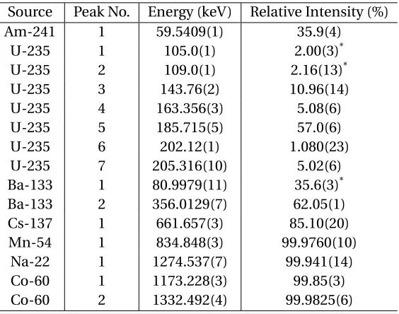
started to become indistinguishable from background beyond that distance. For visual reference, a photograph of the lateral off-axis experimental setup is shown in Figure 3.2.

Figure 3.2Photograph of the HEU disc off-axis experiment 41 cm from the detector and 15 cm to the right (x=+15cm).

3.1. EXPERIMENTAL SETUP CHAPTER 3. EXP. SETUP AND COMP. MODEL

0.32 0.07

0.80

0.16 10

4.76

5.08

ORNL Uranium Disc

1

Noel Nelson

WEIGHT:

Uranium Metal, S.S., Epoxy A4

SHEET 1 OF 1 NOT TO SCALE

DWG NO. TITLE:

REVISION

MATERIAL: DATE SIGNATURE NAME

DEBUR AND BREAK SHARP EDGES FINISH:

UNLESS OTHERWISE SPECIFIED: DIMENSIONS ARE IN CENTIMETERS SURFACE FINISH:

TOLERANCES: +/- 0.005 LINEAR: ANGULAR:

Q.A MFG APPV'D CHK'D DRAWN

3.1. EXPERIMENTAL SETUP CHAPTER 3. EXP. SETUP AND COMP. MODEL

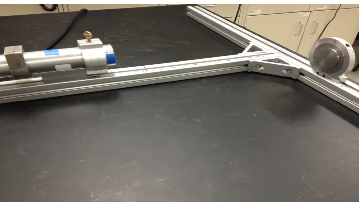
The source in the disc is composed ofU3O8, uranium’s naturally occurring chemical form. The

uranium compound is set on polyethylene epoxy and encased in stainless steel. The activity of the disc was 736µCi on December 1, 2004. However, since uranium-235 has a very long half life (703.8 million years for U-235), the activity of the source at the time of the measurement was similar to its initial activity. The individual uranium nuclides that comprise the disc source employed in our experimental campaign are listed in Table 3.3.

Table 3.3Enrichment of the uranium disc source

Nuclide Weight % U-234 1.016 U-235 93.162 U-236 0.400 U-238 5.421 C (natural) 1.009E-3

The disc is of a high enrichment of U-235. U-235 is a common target material for holdup problems in the nuclear fuel production industry because holdup material deposits present a proliferation risk and can become a criticality safety concern. The typical holdup measurement in this case will seek to detect the naturally emitted low energy gamma radiation. Hence, the focus of the validation experiments has been on the low energies of the detector spectrum where the highest intensity (most probable) gamma rays of U-235 are emitted (140-190 keV). This also explains the choice of the smaller NaI detector size, as high energy detection that would necessitate larger detectors to improve detection efficiency is of lower interest in the holdup field.

3.1. EXPERIMENTAL SETUP CHAPTER 3. EXP. SETUP AND COMP. MODEL

Figure 3.4Photograph of the HEU disc attenuation experiment with two stainless steel plates attached to the detector (11 cm from the source).

3.2. MONTE CARLO TRANSPORT MODELS CHAPTER 3. EXP. SETUP AND COMP. MODEL

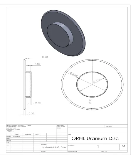
Table 3.4Stainless steel alloy composition used in the MCNP simulations.

Nuclide Weight %

Cr-50 0.800 Cr-52 16.2 Cr-53 0.200 Cr-54 0.400 Mn-55 2.00

Fe-54 4.20 Fe-56 64.8 Fe-57 1.50 Fe48 0.200 Ni-58 6.60 Ni-60 2.50 Ni-61 0.100 Ni-62 0.300 Ni-64 0.100

This composition of steel was taken directly from the MCNP model created by ORNL. The original model is available upon request from the Safeguards & Security Technology Group at ORNL.

3.2

Monte Carlo Transport Models

Version five of the Monte Carlo (MC) code MCNP (Monte Carlo N-Partical Transport Code) was used to calculate the incident gamma-ray photon flux on the 1x2 NaI detector crystal. MCNP is a radiation transport code developed by Los Alamos National Laboratory (LANL) that simulates a large number of random particle histories (particle tracks through a medium as well as collisions with its nuclei) in a user specified geometric configuration according to specified material cross sections (taken from the Evaluated Nuclear Data Files, ENDF). On the order of a few billion particle histories were run for each flux calculation to keep the MC statistical errors smaller than the measurement uncertainties.

3.2. MONTE CARLO TRANSPORT MODELS CHAPTER 3. EXP. SETUP AND COMP. MODEL

apparatuses would be likely to contribute in a small way to the collided fluence tally. There would be no contribution to the uncollided fluence tally as at least one Compton scatter with one of these objects would be required before the particle struck the detector. The detector collimator reduces the likelihood of these events further by reducing the detector solid angle by which particles can strike the detector crystal. So, the secondary geometry (table, tee, etc.) would only make a small contribution to the Compton continuum portion of detector spectra and hence was excluded from the MC models.

With the simplified geometry, an F4 (average fluence) tally was taken in the detector crystal cell by MCNP. MCNP calculates the fluence in a manner very similar to the fluence definition given by Equation 2.1, by summing the particle track lengths over the given cell volume for each discrete energy bin as specified by the user. In our case, 512 equal and discrete energy bins were chosen to match the energy range given by the DRF, and to match the 512 channels observed in the measured spectra. The average fluence tally over cell volume V was approximated discretely as follows,

¯ ΦV(E)'

1 N V∆E

N

X

i=1

ni

X

j=1

W_ijs_ij[ 1

c m2], (3.1)

whereni is the number of times the ith particle enters V at energyEk within energy bin k,s j i is

that particle’s jth track length in V, andW_ij is the particle’s weight when entering V for the jth time. Also, N is the total number of histories simulated by MCNP, and∆E is the width of the tally’s energy bin centered at energy E. This relation is only an approximation of the average fluence, but if a large number of particle histories pass through the cell volume, then it is a fairly accurate tally.[2]

However, as the MCNP fluence is based on the total number of particle histories, it can be converted to a flux as follows

¯

φ(E) =Φ¯V(E)·Aγ[

p h o t o n s

c m2_{·s e c·M e V} ] (3.2)

where A is the activity of the source in Becquerels (Bq) or decays/sec, andγis the yield in particles/decay. So simply multiplying the F4 tally (fluence) by the source activity and yield converts the tally to the approximate scalar flux effective over the volume of the detector crystal.

3.2. MONTE CARLO TRANSPORT MODELS CHAPTER 3. EXP. SETUP AND COMP. MODEL

d N d H =

Z

R(H,E)S(E)d E ≈

G

X

i=1

RG(H,Ei)φ¯(Ei)εa b s(Ei). (3.3)

The formal definition from Knoll is listed first and is approximated by the more directly applicable second definition. R(H,E) is the differential probability that a quanta of energy within dE about E leads to a pulse with amplitude within dH about H (DRF). S(E)dE is the differential number of incident radiation quanta with energy within dE about E.[9]RG(H,Ei)is Gardner’s DRF, which is the

differential probability that a flux of energyEi leads to a pulse with amplitude within dH about H

(DRF), andεa b s(Ei)is the absolute efficiency. ¯φ(Ei)is the flux. To fully determine a detector response

using Gardner’s model, a new quantity must be defined and calculated: absolute efficiency. Detector efficiency in general determines the percentage of radiation particles detected to the number emitted. There are two main classes of detector efficiency, absolute efficiency and intrinsic efficiency. Knoll defines absolute efficiency as simply the ratio of the number of detector pulses recorded to the number of particles with energy E emitted from the source. Absolute efficiency is dependent mainly on detector properties (cross-sections) and the counting geometry (source to detector position). Whereas the intrinsic efficiency is the ratio of the number of detector pulses recorded to the number of radiation quanta incident on the detector. The intrinsic efficiency is accounted for by the DRF, however, the absolute efficiency is not. Therefore it must be approxi-mated as the energy deposited along the average path length through the detector crystal in MCNP simulation.[9]

In other words, the total absolute efficiency is the probability of particles incident on the detector interacting with the detector crystal over all energies (thereby creating a pulse at energy E). This probability is defined as

εj

a b s(E) =Pi n t e r a c t i o n=1−e−µt o t(E)·sj(E) (3.4)

whereµt o t(E →E0,Ω→Ω0)is the NaI photon macroscopic cross section and probability that an

incident particle of energy E interacts per unit path length.s_j(E)is the track length and an MCNP program called ptrac was used to record a large number of possible particle track lengths. This distribution was then averaged over all track lengths to produce an average absolute efficiency

¯

εa b s(E)as shown in Equation 3.5.

¯

εa b s(E) =

1 Nt

Nt

X

j=1

εj

a b s(E) (3.5)

3.2. MONTE CARLO TRANSPORT MODELS CHAPTER 3. EXP. SETUP AND COMP. MODEL

CHAPTER

4

VALIDATION

Overall, the simulated detector responses predicted by Gardner’s model predicted the highest intensity peak region of the experimental spectra fairly well, but had some difficulty in the continuum and secondary peak regions. In the highest intensity peak region of the response, most of the computed spectrum lay within two standard deviations of the experimental spectrum’s centroid. The continuum discrepancies between the predicted and measured responses in the calibration sources appear to stem from miscalibration of the electron range multiplier (Equation 2.4) for the collimated 1x2" NaI detector. Gardner’s current model was validated only for larger bare NaI detectors and not for collimated detectors and therefore some differences were expected. Whereas, significant underestimation of the secondary peaks occurred in the highly enriched uranium (HEU) disc spectra most likely due to outside crystal scattering with the detector collimator and other components.

4.1

Cs-137 Measurement

4.1. CS-137 MEASUREMENT CHAPTER 4. VALIDATION

percent uncertainty in the peak region in terms of counts (according to Poisson counting statistics), and it was counted for 4000 seconds. This source was used for validation and as one of the data points for the power law fit but not for the final energy calibration. The resulting spectra computed and measured are given in Figure 4.1a and compared with the computed response without the lead collimator and aluminum sheath simulated in the MCNP flux calculation (Figure 4.1b).

0.2 0.3 0.4 0.5 0.6 0.7 Energy (MeV) 10-3 10-2 10-1 100 101 102 103 104

Count Rate (cps)

Cs-137 Source at 10 cm

normalization bounds measured response normalized computed response two sigma confidence interval

(a)

0.2 0.3 0.4 0.5 0.6 0.7 Energy (MeV) 10-3 10-2 10-1 100 101 102 103 104

Count Rate (cps)

Cs-137 Source at 10 cm

normalization bounds measured response normalized computed response two sigma confidence interval

(b)

Figure 4.1Measured and normalized computed responses for the Cs-137 calibration source at 10 cm (normalized across bounds) with aluminum can (a) and without aluminum can and collimator (b).

It is apparent that the backscatter peak is overestimated and the peak underestimated. However, the greatest difference lies in the area between Compton edge and the peak, which will henceforth be referred to the valley of the response. At first this effect was thought to be just a product of the model being unable to account for the collimator geometry. In Sood’s PhD thesis, a similar problem was occurring in the valley region of the response for their NaI 3x3" detector. However, the effect was reversed. For a bare NaI crystal simulation in MCNP for the flux calculation, the resulting response underestimated the valley. Simulating the detector aluminum sheath or can corrected this underestimation.[12]

4.1. CS-137 MEASUREMENT CHAPTER 4. VALIDATION

Another difference between this validation exercise and Gardner and Sood’s validation exercises, was how the computed spectrum was normalized to the measured response. Gardner and Sood chose to normalize to the peak channel only, whereas in this work, normalization to the area under the section of interest bounded by the normalization bounds was chosen instead. The normal-ization factor used to normalize the computed to the measured response spectrum is described mathematically by Equation 4.1

Ac = nb2 X

nb1 R_ic,

Am= nb2 X

nb1 R_im,

N_f =Am Ac

, (4.1)

whereR_ic is the computed count rate, andR_imis the measured count rate at channel i.nb1and

nb2are the normalization bounds. Normalization bounds were chosen on a case by case basis. In

this case the bounds were chosen to avoid bins artificially augmented by the rebinning process and unnecessary noise after the full energy peaks. Rebinning was accomplished by assuming the count rates within the old bins were uniformly distributed, and then collecting them into the new bins according to the fractions of the old bins determined by the uniform pdf. All contribution from the negative energy bins created from the energy calibration were lumped into the first two bins by the rebinning algorithm. Therefore those two bins were not included in the normalization.

4.2. CO-60 MEASUREMENT CHAPTER 4. VALIDATION

0.2 0.3 0.4 0.5 0.6 0.7 Energy (MeV)

10-3 10-2 10-1 100 101 102 103 104

Count Rate (cps)

Cs-137 Source at 10 cm

normalization bounds measured response normalized computed response two sigma confidence interval

(a) (b)

Figure 4.2(a) Measured and normalized computed responses for the Cs-137 calibration source at 10 cm (normalized to the peak). (b) 3x3" NaI detector computed responses over a varying electron range multi-plier compared with the measured response from the Heath benchmark.

Now, as can be seen, the whole response spectrum is overestimated to the left of the peak for the figure on the left. A similar effect is observed by a spectrum with an electron range factor that is too low in Gardner’s figure (right).[16]A range multiplier that is too high underestimates the continuum and a valley, while the reverse is true for one that is too low. Since the size of the detector and number of channels of the 1x2" ORNL detector is very different from Gardner’s detector it is not surprising that the value of the electron range multiplier may no longer be optimal. Furthermore, the psuedo-electron range multiplier (Equation 2.4) was fit for Gardner’s detector by trial and error. For this reason, and the fact that the HEU spectrum of interest contains far less contribution from Compton scatter, the correction of the factor is reserved for future work.

4.2

Co-60 Measurement

4.2. CO-60 MEASUREMENT CHAPTER 4. VALIDATION

and a simple baseline validation (shown in Figure 4.3a). The energy calibration and its parameter uncertainties are discussed further in Section 5.2.

0.2 0.4 0.6 0.8 1.0 1.2 1.4 Energy (MeV) 10-3 10-2 10-1 100 101 102 103 104

Count Rate (cps)

Co-60 Source on Detector Face

normalization bounds measured response normalized computed response two sigma confidence interval

(a)

0.2 0.4 0.6 0.8 1.0 1.2 1.4 Energy (MeV) 10-3 10-2 10-1 100 101 102 103 104

Count Rate (cps)

Cs-137 Source at 10 cm

normalization bounds measured response normalized computed response two sigma confidence interval

(b)

Figure 4.3(a) Measured and normalized computed responses for the Co-60 calibration source on the detector face using normalization across a range of channels (a) and normalized to the highest intensity peak (b).

As expected, the measured spectrum shows some significant fluctuation in the confidence interval along the response due to the low number of counts (higher uncertainty). The normalized computed response stays mostly well within the confidence interval of the measured response except at the backscatter peak around 2 MeV and the peaks are slightly underestimated. The two Compton edges and most of the continuum are predicted fairly well, however the backscatter peak region around 0.2 MeV is overestimated and the full energy peaks are slightly underestimated.