ABSTRACT
MUELLER, KATELYN ELIZABETH. Using Life Cycle Assessment and Environmental
Payback Period to Evaluate Commercial Building Replacement. (Under the direction of Drs.
Joseph DeCarolis and Jeremiah Johnson).
As environmental and human health impacts garner more global concern, buildings
represent near-term opportunities to mitigate impacts cost-effectively. Environmental payback
period (EPP) is an existing metric that applies the concept of economic payback period to
environmental impacts. This project investigates the application of an EPP methodology to
commercial buildings to make recommendations regarding building replacement, informing
the point at which existing, underperforming buildings should be replaced with new,
high-performing ones.
The EPP estimation model developed in this work includes the application of life cycle
assessment (LCA) to generate an emissions inventory that includes building construction and
operation. The inventory is used to calculate environmental impacts, which are in turn used to
estimate the EPP by impact category. The model is capable of applying variations in discount
rate and energy efficiency. While global warming potential is frequently used as the benchmark
for the environmental performance of buildings, this project also seeks to determine if other,
often unassessed impact categories may be areas of concern for building projects, indicated by
high EPPs. The selected case study is a college administrative building.
Using Life Cycle Assessment and Environmental Payback Period to
Evaluate Commercial Building Replacement
by
Katelyn Elizabeth Mueller
A thesis submitted to the Graduate Faculty of
North Carolina State University
in partial fulfillment of the
requirements for the degree of
Master of Science
Civil Engineering
Raleigh, North Carolina
2018
APPROVED BY:
_______________________________
_______________________________
Dr. Joseph DeCarolis
Dr. Jeremiah Johnson
Committee Co-Chair
Committee Co-Chair
DEDICATION
ii
BIOGRAPHY
Katelyn Mueller was born in Wilmington, NC in 1994. She is the eldest child of Peter and
Suzanne Mueller, with younger brothers Matthew and Alexander. Having lived in five states
as a child, her earliest memory is of a tornado in Ft. Leavenworth, Kansas, but other formative
experiences include a smattering of broken bones, stitches, rec sports, and countless visits to
national parks and historic sites. Upon graduating from Robinson Secondary School in Fairfax,
Virginia in 2012, she enrolled at North Carolina State University.
Coming from a long line of civil engineers and surveyors, Katelyn did her best to avoid
the family trade, yet completed her Bachelor of Science in Civil Engineering and the University
Honors Program at NC State in 2016. She decided to continue her education by pursuing a
master’s degree through which she could further explore the environmental implications of the
built environment.
iii
ACKNOWLEDGMENTS
I would first like to acknowledge my advisor, Dr. Joe DeCarolis, for the instrumental role
he played in the completion of this thesis. I am truly grateful for his support and guidance
throughout this process, beginning with his willingness to help me develop and pursue a project
of my own interest. As I entered graduate school I was aware of my passions, yet had only a
foggy vision of what I ultimately wanted from a career. Thank you for taking the time to help
me examine potential pathways, and for assisting me in pursuing opportunities as I came upon
them throughout my graduate program.
Additional thanks to Dr. Jeremiah Johnson for his willingness to join my committee
midway through this project, shortly after arriving at NC State. I greatly appreciate all of your
valuable insights and suggestions. I would also like to acknowledge Dr. Ranji Ranjithan for
both serving on my committee and cultivating my appreciation for challenging problems with
an array of viable solutions.
Many thanks to John Majernik at Wake Tech Community College and Candis Parker at
Balfour Beatty Construction for their interest in this project and providing the data that made
it possible.
There are numerous others without whom the completion of this thesis – at least a remotely
graceful completion of this thesis – would not have been possible:
iv
To my Fellowship Raleigh Church family: thank you for your care and support, and for
serving as a lay-audience as I practiced presenting and communicating my research.
To my parents, brothers, and extended family: thank you for encouraging me to take on
new challenges, for celebrating the milestones with me, and for never failing to communicate
to me that you are proud of my efforts and accomplishments. I love you all and am fortunate
to have such great examples in my life.
To Hannah Field: thank you for your friendship, and for being an incredible example of
how to support and encourage others – both in person and from a number of states away.
To my friends and compatriots in Mann Hall, particularly those on the fourth floor: thank
you for the laughs, the trivia victories, and for being a light in our shared windowless box.
v
TABLE OF CONTENTS
LIST OF TABLES ... vii
LIST OF FIGURES ... viii
1
INTRODUCTION ... 1
2
MATERIALS AND METHODS ... 6
2.1
Existing Tools and Techniques ... 6
2.1.1
Life Cycle Assessment ... 6
2.1.2
Payback Period ... 7
2.1.3
Environmental Payback Period ... 8
2.2
EPP Framework and Case Study ... 10
2.2.1
LCA Application ... 11
2.2.2
Case Study ... 13
2.2.3
Model Structure & Data ... 13
2.2.4
Base Comparison ... 16
2.2.5
Energy Reduction ... 17
2.2.6
Discount Rate ... 17
2.2.7
Variation in Material Selection ... 18
2.2.8
Variation in Electricity Supply ... 18
2.2.9
Building Efficiency... 21
2.2.10
Spreadsheet Function ... 22
3
RESULTS AND DISCUSSION ... 24
3.1
Base Comparison ... 24
3.2
Energy Reduction... 26
3.3
Discount Rate ... 28
3.4
Interaction of Energy Reduction and Discount Rate ... 31
3.5
Variation in Material Selection ... 33
3.6
Variation in Electricity Supply ... 34
3.7
Building Efficiency ... 37
4
IMPLICATIONS ... 39
4.1
Green Building Rating Context ... 39
4.2
Shortcomings of EPP ... 40
4.3
Comparison to Existing Literature ... 41
4.4
Other Temporal and Discount Rate Considerations ... 43
vi
5.1
Role of Demolition and Recycling Methods ... 45
5.2
Consideration of Renovation and New Construction ... 47
5.3
Changes to Annual Energy Reduction ... 49
6
CONCLUSION ... 49
REFERENCES ... 51
APPENDIX ... 56
Appendix A1 New Building Materials ... 57
Appendix A2 Energy Consumption Data ... 58
vii
LIST OF TABLES
Table 1.
Differences in impacts per kWh for manual and Ecoinvent SERC
representations ... 20
Table 2.
Impact ratios for 25% energy reduction and 0% discount rate ... 30
Table 3.
Percent change in EPP due to 25% decrease in material input ... 33
Table A1.
Materials included in representation of new building construction ... 57
Table A2.
Existing building annual electricity use ... 58
Table A3.
Existing building annual fuel oil use ... 58
Table A4.
New building monthly electricity use ... 58
Table A5.
Projected generation contributions by fuel type for SERC - AEO 2017
Reference ... 60
viii
LIST OF FIGURES
Figure 1.
LCA framework diagram.. ... 7
Figure 2.
Graphical representation of environmental payback period (EPP) applied to
buildings. ... 9
Figure 3.
Environmental payback period (EPP) model workflow. ... 10
Figure 4.
System boundary diagrams for existing and new buildings. ... 12
Figure 5.
Base case environmental payback periods, normalized impacts from initial
construction, and normalized 50 year cumulative impact savings. ...25
Figure 6.
Percent energy reduction versus environmental payback period for TRACI
impact categories. . ... 27
Figure 7.
Percent discount rate versus environmental payback period for TRACI
impact categories.. ... 29
Figure 8.
Environmental payback period and normalized 50 year cumulative impact
savings when percent energy reduction and discount rate are varied
simultaneously.. ... 32
Figure 9.
Effect of grid transition over time on environmental payback period. ... 35
Figure 10.
Effect of 100% solar electricity supply on environmental payback period
when applied to just the new building and to both buildings. ... 36
Figure 11.
Comparison of changes to energy efficiency required to eliminate payback
1
1
INTRODUCTION
2
have emerged to provide high performance building standards and evaluate building
sustainability, including Leadership in Energy and Environmental Design (LEED), WELL
Building Standard (WELL), the Living Building Challenge, and ASHRAE 189.1 (Green
Building Alliance, 2016; Mukhopadhyay, Baltazar, Kim, & Haberl, 2011; Zuo & Zhao, 2014).
While improved certification scores do not guarantee decreased environmental impacts,
studies have quantified the benefits of building certifications, particularly increased energy
efficiency in LEED certified buildings. The energy reduction achievable by high performance
buildings varies, though LEED buildings are demonstrated to produce energy reductions of 10
to 44% when compared to conventional construction (Newsham, Mancini, & Birt, 2009; Suh,
Tomar, Leighton, & Kneifel, 2014; Turner & Frankel, 2008). ASHRAE 189.1 (Standard for
the Design of High Performance Green Buildings) targets 30% less energy consumption than
ASHRAE 90.1 (Standard for Buildings Except Low-Rise Residential Buildings) (Suh et al.,
2014). In addition to energy-related savings, benefits of green buildings include increased
urban biodiversity (Henry & Frascaria-Lacoste, 2012) and improved construction and
demolition waste management (Yeheyis, Hewage, Alam, Eskicioglu, & Sadiq, 2013).
3
Though high performance buildings are the beneficiaries of real or perceived environmental
benefit when compared to conventional buildings (Holmgren, Kabanshi, & Sörqvist, 2017), a
life cycle approach is required to justify such claims and may reveal areas of environmental
concern.
Heterogeneity in building characteristics can make building-focused LCA difficult,
frequently limiting its use to the assessment of single building projects. However, there are
many situations that involve sets of building stock, such as in municipal or institutional
settings, where entities are faced with decisions about how to manage many buildings as they
age and ultimately need to be renovated or replaced. Numerous factors inform such decisions,
including cost, resource availability, and cultural or historic significance (Thomsen & van der
Flier, 2009), but environmental metrics are increasingly important as cities and institutions
adopt environmentally-oriented goals or targets.
4
environmental impacts assessed do not have a specific focus on ecosystems, organisms, and
biodiversity.
Previous studies have adopted the payback period concept for carbon emissions, coined
“carbon payback period”, most of which pertain to the carbon emissions associated with
renewable energy production. For example, Gibbs et al. (2008) investigate the carbon payback
time for biofuel production in tropical regions, Jonker et al. (2014) assess wood pellet
production in the southeastern US, and Lu and Yang (2010) assess greenhouse gas payback
time for solar photovoltaic systems in Hong Kong.
Faludi and Lepech (2012) extend the environmental payback period methodology to
buildings. Their analysis of a prefabricated modular building includes payback for both carbon
and the overall impact score from EcoIndicator 99, a damage-oriented impact assessment
methodology, and finds payback times to be on the order of years, not decades. As the first and
only study thus far to apply EPP to buildings, it provides insights into the potential
environmental benefits of building replacement projects. However, their study was not
designed to thoroughly examine EPP as a methodology, identify key contributing factors to
EPP, or determine EPP per impact category, all of which are areas that warrant further
investigation.
5
contributors to each impact. To generate a tool that can rapidly estimate EPP for a set of
buildings, it is necessary to determine what factors affect EPP and should be included in such
a model. The goal of this work is to identify the conditions under which it is environmentally
advantageous to replace an existing building and the environmental impacts most affected by
the transition. The project also seeks to quantify the conditions under which an existing,
underperforming building should be replaced with new, high performance construction and
how long it takes for the environmental benefits of the new building to surpass the impacts
from its construction.
Use of EPP as a metric could simplify the application of LCA in the building community,
thereby reducing the complexity and difficulty of interpretation (Saunders et al., 2013). A
refined EPP calculation methodology could ultimately be extended to a tool to enable the rapid
estimation of EPP for a set of commercial, institutional, or municipal building stock. A shorter
EPP would flag a building as a potential candidate for replacement. Such a screening tool could
identify particular building replacement projects that provide the greatest environment benefits
and highlight them as high priority, allowing engineers and planners to conduct further
assessments of cost, energy savings, and economic payback to determine the viability of
replacement. This targeted approach would help prioritize efforts related to redevelopment, as
large scale turnover of buildings is likely to be cost and resource prohibitive.
6
2
MATERIALS AND METHODS
2.1
Existing Tools and Techniques
2.1.1
Life Cycle Assessment
Life cycle assessment is an established methodology for quantifying the environmental
impacts associated with a product or process. As defined by the International Organization for
Standardization (ISO) 14040, LCA is a “compilation and evaluation of the inputs, outputs and
the potential environmental impacts of a product system throughout its life cycle”
(International Organization for Standardization, 2006a). Guidance on how to conduct LCA is
established by the ISO 14040 and 14044 standards, which describe the principles and
framework for LCA, as well as requirements and guidelines (International Organization for
Standardization, 2006b). The International Reference Life Cycle Data System (ILCD)
handbook produced by the European Commission provides further guidance on performing
LCA and conforms to the ISO standards (European Commission Joint Research Centre, 2010).
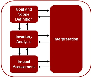
LCA consists for four major stages, as illustrated in Figure 1.
Figure 1. LCA framework diagram. The arrows between stages in the framework highlight the importance of iteration and interpretation throughout the process to revise and refine the analysis.
7
the collection and documentation of data. This involves quantifying inputs and outputs
associated with each process within the system boundary and relating them to the functional
unit. The impact assessment stage maps the emissions inventory to a more limited set of impact
categories, such as global warming potential or acidification, aiding in interpretation. As LCA
is an iterative process, interpretation happens throughout the analysis to refine or revise aspects
of the previous steps and ultimately produce insights about the system and make
recommendations.
Climate change related impacts, specifically carbon emissions and carbon dioxide
equivalents, are a commonly used impact category for benchmarking environmental impacts
associated with buildings due to their correlation to energy consumption (C. Peng, 2016; Seo
& Hwang, 2001). However, databases used in LCA include inventory items that address a wide
range of impact categories, and an extensive body of LCA studies on various topics has also
focused on other impacts such as acidification or ozone depletion. Climate change related
impacts do not capture the full range of impacts generated by buildings over their life cycle,
motivating the consideration of other impact categories in building-related studies.
2.1.2
Payback Period
One of many metrics used in the process of making capital investment decisions is
payback period. This is an economic metric that estimates the time required for an investment
to recoup initial costs through annual savings (Weingartner, 1969). For example, the decision
to purchase a piece of machinery rather than lease it could be analyzed via payback period.
Mathematically, payback period represents the point at which Equation 1 is satisfied.
𝐶
0= ∑
𝐶𝑡
(1+𝑟)𝑡
𝑇
8
In Equation 1,
C
0is the investment at time 0,
C
tis the revenue at time
t, and
r is the
discount rate. Solving for t produces the payback period, as shown in Equation 2.
𝑡 =
log ([1−𝐶0 𝐶𝑡𝑟]
−1
)
log(1+𝑟)
(Eq. 2)
While payback is not a comprehensive metric on which investment decisions should be
made, it allows for a simple comparison of alternatives. It can also serve as a constraint for
investment selection; an investor may choose to only select projects that have paybacks shorter
than a designated period of time. The primary shortcoming of this metric is that is does not
address the magnitude of the payback. While a payback may be short, the magnitude of cost
and savings could also be small. Therefore, alternatives with the same payback period could
produce markedly different savings in absolute terms.
2.1.3
Environmental Payback Period
The concept of payback period has been extended to other quantities, such as energy. In
this case, the applicable metric is energy payback, or the point of time at which an energy
technology, such as a solar photovoltaic panel, produces as much energy as was consumed
throughout
the product
lifecycle, including manufacturing, transportation, and
decommissioning (Lu & Yang, 2010; J. Peng et al., 2013).
The combination of both LCA and payback period principles produces the metric of
environmental payback period. Instead of using capital or energy as investments to be
reconciled, the framework determines the point at which initial environmental impacts
associated with a product or system are equivalent to the environmental impact savings
accumulated by use of the product when compared to a conventional alternative. When
Equations 1 and 2 are applied to EPP in buildings, C
0then becomes representative of initial
9
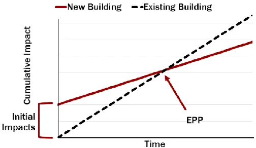
between the annual impacts from the existing and new buildings. The new building is assumed
to have lower operational impacts, creating these savings.
LCA is used to estimate the environmental impacts, which are then utilized within the
payback methodology. Figure 2 illustrates a simplified graphical representation of
environmental payback period.
Figure 2. Graphical representation of environmental payback period (EPP) applied to buildings. The slope of each line represents annual operational impacts. The new building incurs initial impacts from construction activities, but its lower operational impacts due to improved efficiency enable the initial deficit to be recovered.
10
2.2
EPP Framework and Case Study
The EPP model used in this study is designed to evaluate the replacement of commercial
buildings of comparable size and function. Commercial buildings are selected due to their
prevalence and similar use phase characteristics. While renovations and retrofits can improve
building performance, this analysis focuses on replacement scenarios. Given the large number
of building elements that are candidates for retrofits, this research represents an approach that
could later be extended to renovation projects. This EPP model requires the characterization
of a business-as-usual case involving the continued operation of the existing building, and the
characterization of the construction and future operation of a new building. Both life cycle
assessment and payback principles are utilized in this application. This is a multistep process,
as illustrated by Figure 3.
Figure 3. Environmental payback period (EPP) model workflow. Energy and material data for existing and new buildings are compiled in a life cycle assessment (LCA) model database. Impact assessment is applied using the Tool for Reduction of Chemical and Other Environmental Impacts (TRACI) method, and impact assessment results are transferred to a spreadsheet model from which EPP is calculated.
11
contains data on both initial construction and operational impacts, and is used to perform the
payback calculation and related sensitivity analysis. This is discussed further in Section 2.2.3.
Impact assessment is conducted using the Tool for Reduction of Chemical and Other
Environmental Impacts (TRACI), developed by the U.S. EPA. TRACI includes 10 impact
categories capturing both environmental and human health factors (Bare, Young, Qam,
Hopton, & Chief, 2012). The use of all ten impact categories yields a more comprehensive
assessment of building-related impacts when compared to global warming potential alone.
Impact assessment results are entered into the spreadsheet model, where variables such as
discount rate and energy efficiency changes are altered and EPP is determined.
2.2.1
LCA Application
12
Figure 4. System boundary diagrams for existing and new buildings. The model calculates existing building impacts based on energy use, while the model can incorporate demolition, construction, and operational components for the new building impacts. In this study, however, demolition impacts are not included in the EPP calculation.
The system includes construction and operation and excludes demolition as described in
Section 2.2.3. Processes and flows are developed on the whole-building scale. Instead of
calculating the required materials per square foot in building construction, the total quantities
are input and the impact assessment outputs are then divided by the building square footage to
produce impact per functional unit.
13
factors used in the project are based on TRACI 2.1 normalization factors, which are derived
from Ryberg et al. (2014) and are based on 2008 data for the United States.
2.2.2
Case Study
This analysis uses a newly constructed, LEED certified classroom and administrative
building at Wake Tech Community College (WTCC) as the case study for application of the
EPP framework. Located in Raleigh, North Carolina, the four story, approximately 49,000 ft
2building was completed in 2014 and serves the functions of its predecessor, an approximately
48,000 ft
2building on the campus. The building is oriented on a roughly north-south axis and
has a predominantly glass façade. The administrative function of the building closely matches
the usage of commercial buildings, and does not include specialty lab space or other functions
that may be unusually energy intensive.
2.2.3
Model Structure & Data
The building characterization and model structure includes aspects of building operation
of both the existing and new building, as well as construction of the new building. Demolition
impacts are not included in the EPP calculations.
2.2.3.1
Construction
14
The construction materials inventory is developed based on the bill of materials for the
building, which was obtained from the project contractor. A previous building LCA study by
Thiel et al. (2013) was consulted to determine what material elements to include. Elements of
the concrete work, structural and miscellaneous metals, roofing, glass and frames for windows,
drywall, flooring, ceiling tiles, plumbing, and HVAC material groups are included. The study
does not include sitework (i.e., excavation, site utilities, paving, landscaping, signage) or
finishing details (i.e., cabinets, fixtures, doors and hardware, paint, furnishings, electrical). The
complete list of materials included in the LCA model can be found in Appendix A1 New
Building Materials.
2.2.3.2
Operation
The operational component of the model captures the environmental impacts associated
with annual energy consumption. This applies to both the existing and new building cases.
This component does not account for periodic renovation or maintenance requirements, water
use, or materials consumed for tasks carried out in the building, such as cleaning products,
office supplies, or appliances.
15
2.2.3.3
Demolition
Demolition processes consider the destruction of a building and transport of resulting
wastes to landfill and/or recycling facilities (Cabeza et al., 2014). Often, demolition is
considered but not fully quantified in building LCA due to the greater ability to reduce impacts
and energy use by making changes in the operational life of buildings (Biswas, 2014; Wang,
Shen, & Barryman, 2011). When included, studies demonstrate minor contributions to overall
lifecycle impacts (Kofoworola & Gheewala, 2008; C. Peng, 2016). Additionally, limited
empirical data on demolition processes exists (Scheuer et al., 2003). Outside the LCA
literature, demolition has been considered in the context of waste management in a number of
studies (Bergsdal, Bohne, & Brattebø, 2007; Ding & Xiao, 2014; Seo & Hwang, 1999; Wu,
Yu, Shen, & Liu, 2014). This body of work does not specifically address environmental
impacts, but estimates construction and demolition (C&D) waste for a number of buildings of
different vintages, location, and types. The studies develop sets of waste characterization
factors by which quantities of material wastes can be estimated based on different building
parameters. Such studies serve to determine the load that demolition places on the waste
management system, and burdens associated with waste handling. Waste characterization
factors can be used in the context of the EPP calculation by using properties of the existing
building to estimate the amount of waste associated with the building demolition.
16
4% of CO
2emissions from demolition (C. Peng, 2016; Suzuki & Oka, 1998). Further
qualitative demolition implications, including the allocation of impacts between existing and
new building, are considered in Section 5.1.
2.2.4
Base Comparison
All power needs in the new building are supplied by grid electricity, while the existing
building was served by grid electricity supplemented with fuel oil for heating. In this analysis,
the existing building energy use was converted to electricity to make a simplified comparison
with the new building based strictly on electricity consumption. After making this conversion,
the new building was found to use more primary energy than the existing building, and, as a
result, the EPP model did not find a payback for any impact categories. This may be attributed
to increased building usage as the new building is more inviting and provides greater occupant
comfort than the original building, or an introduction of increased plug loads and other
technology. To create a scenario in which paybacks can be investigated, a 25% energy
reduction between the existing and new building is selected to represent the base case
comparison. This value is selected based on existing work that studied the energy performance
of LEED and other high performance buildings. Turner and Frankel (2008) found buildings
constructed using LEED for new construction guidelines require an average of 28% less energy
when compared to the US national average.
17
2.2.5
Energy Reduction
To quantify the effect of new building energy savings, a range of 0 to 50% energy
reduction between the existing and new buildings is implemented by adjusting the primary
energy inputs in OpenLCA and transferring the resulting adjusted operational impacts to the
EPP model.
2.2.6
Discount Rate
In economics, discount rates are rates applied to future cash flows to determine their
present value, enabling comparisons of cash flows that occur at different times. The
interest-earning potential makes money more valuable today, which means that the present value of
future cash flows is less than or equal to the future value, subtracting out interest. The
environmental payback model enables application of a discount rate to quantify the relative
value of future impacts at the present time.
18
promote intergenerational equity by considering future generations, and place burdens on
current emitters rather than members of future generations.
When considering what may affect EPP, analysis is not only concerned with building
performance, but how the environmental effects of the performance are valued. There is much
deliberation about whether or not to discount environmental impacts and to what degree. A
discount rate analysis is performed by varying the discount rate input into the EPP model
within the range of -8 to 8%. Positive discount rates imply valuing future impacts less than
impacts incurred today, whereas negative values imply valuing future impacts more than
impacts incurred today.
2.2.7
Variation in Material Selection
Changes to building material quantities are conducted to investigate how the materials
used in new construction affect EPP. Building material quantities are individually decreased
by one percent to determine the percentage change in each building impact category. This is
done to individual materials (e.g., copper), as well as building systems (e.g., HVAC). The top
five materials producing the largest change for each impact category are chosen for further
investigation using EPP. A 25% reduction in each selected material is implemented to
determine the corresponding change to EPP. A reduction of 25% is selected to induce a change
large enough to affect EPP and assess the relative impact of different materials in the model.
This is done by altering the material inputs in OpenLCA and updating the construction module
in the EPP model to reflect the new impacts associated with the material changes.
2.2.8
Variation in Electricity Supply
19
buildings will also change. While this is a factor that building owners or occupants may not
necessarily have control over, it could still affect the future environmental benefits associated
with their facilities. An assessment of different electric grid mixes and the evolution of the grid
mix over time can determine whether the same benefits anticipated with the current grid mix
will stay the same, reduce, or increase given grid changes.
20
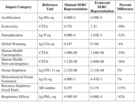
Table 1. Differences in impacts per kWh for manual and Ecoinvent SERC representations
Impact Category
Reference
Unit
Manual SERC
Representation
Ecoinvent
SERC
Representation
Percent
Difference
Acidification
kg SO
2eq
6.80E-4
6.50E-4
5%
Ecotoxicity
CTUe
0.752
1.21
-38%
Eutrophication
kg N eq
8.00E-4
1.65E-3
-52%
Global Warming
kg CO
2eq
0.187
0.196
-4%
Human Health -
Carcinogenics
CTUh
1.09E-08
1.69E-08
-35%
Human Health –
Non-carcinogenics
CTUh
3.12E-08
4.89E-08
-36%
Ozone Depletion
kg CFC-11 eq
2.21E-08
2.11E-08
5%
Photochemical Ozone
Formation
kg O
3eq
4.80E-3
4.47E-3
7%
Resource Depletion -
Fossil Fuels
MJ surplus
0.255
0.119
115%
Respiratory Effects
kg PM
2.5eq
4.99E-05
6.00E-4
-92%
There are a number of discrepancies between the Ecoinvent data, manual SERC data, and
powerplant emissions data obtained from the EPA Emissions and Generation Resource
Integrated Database (eGRID). This may be attributed to resource variability between SERC
sub-regions or data vintage. As the US energy grid rapidly transitions away from coal in some
areas of the country, associated environmental impacts will also change from year to year.
Thus, results produced here are illustrative of the implications of a cleaner grid, but may not
closely match the reality of the current SERC grid.
21
Plan (CPP) is an Obama-era framework setting state-level limits on carbon emissions from
power plants. It enables state-level implementation plans and seeks to promote renewable
energy generation and energy efficiency (The White House, 2015). Though implementation is
on hold as the EPA proposed to repeal the CPP in 2017 (EPA, 2017a), the CPP scenario
represents a potential lower-carbon energy pathway, and many states are well-positioned to
meet emissions targets despite the absence of federal-level policy (Plumer & Popovich, 2017).
Year 1 of the model is set at 2016, the first year of the AEO case, and is updated with grid
mix changes in five year increments beginning with 2020. After 2050, the grid mix is assumed
constant in the absence of further AEO estimates for both scenarios. While the AEO Reference
Cases provide insights into grid-level changes, this study also considers on-site energy
generation. This is simulated through on-site solar power adoption for which SERC electricity
was replaced with 100% solar photovoltaics. These scenarios are applied to (1) both buildings
and (2) the new building only, in which case the existing building receives all electricity from
the SERC grid. For grid transition cases, the updated electricity supply is implemented by
adjusting resource quantities in the manual SERC mix in Ecoinvent and transferring the impact
results to the operations module of the EPP model, and the solar cases utilize the AEO 2016
Reference Case values.
2.2.9
Building Efficiency
22
the new building and the existing building. The user may input a unique percentage value for
both the existing and new buildings, representing an annual anticipated change in energy
consumption. This simulates how building owners or occupants can undertake energy
efficiency projects and improve energy consumption over time, or how buildings begin use
more energy as systems become less efficient, lack proper operations and maintenance, or plug
loads are added. This approach is taken for simplicity and flexibility, and percent reductions
are not tied to a specific technology choice or energy reduction strategy.
This functionality is included to determine how closely realized building performance
must conform to the projected performance of the design to achieve the anticipated
environmental benefit, captured in terms of EPP. Similarly, the effect of energy efficiency
improvements to an existing building on EPP is also considered. Changes are modeled by
varying the increases in efficiency for the existing building and decreases in efficiency for the
new building in the EPP model. These values are incrementally changed to examine the point
at which each impact category no longer pays back, thus determining which impact categories
are most sensitive to such operational changes. Increases to existing building efficiency and
decreases to new building efficiency are varied separately (e.g., existing building efficiency is
varied with new building efficiency held constant). These changes are not tied to specific new
materials or systems and their associated impacts.
2.2.10
Spreadsheet Function
23
are considered. The model defaults to assigning construction impacts and existing building
operational impacts to the first year in the model, with new operational impacts beginning in
Year 2. This accounts for the fact building occupants will need to be housed during the new
building construction, producing operational impacts during that time. As with the existing
building, the same operational impacts are assigned to each subsequent year in the model. From
a decisionmaking perspective, this captures the impacts associated with the site on which the
replacement project takes place in the business-as-usual and new building cases.
Changes to energy efficiency alter the operational stage environmental impacts. The
calculation is included in Equation 3, where I is the annual environmental impact for a specific
impact category, n is the year, and
ΔE is the annual improvement in energy use, given as a
percentage:
𝐼
𝑛+1= 𝐼
𝑛∗ (1 −
∆𝐸100
)
(Eq. 3)
Thus, if energy use improves by 0.5% annually, the environmental impacts will decrease
by 0.5% annually. After energy use adjustments are made, the model applies a discount rate
and determines cumulative discounted impacts using Equation 4, where
P is the cumulative
“present worth” of impacts, I
nis the impacts occurring in year n, and i is the discount rate:
𝑃 = ∑
𝑁𝐼
𝑛(1 + 𝑖)
−𝑛𝑛=1
(Eq. 4)
24
In addition to EPP, the normalization of cumulative 50 year impacts to person-equivalents
serves as a benchmark for building performance. Negative normalized values indicate
cumulative impact savings, or avoided impacts, while positive values indicate an increase in
impact from the new building when compared to the existing building. While EPP produces
an easy to understand means of comparison, normalized impacts enable assessment of impact
magnitude and more insightful interpretations when used in conjunction with EPP. For
example, an impact category with a short EPP but a small normalized magnitude would
indicate that the change is not especially impactful, while a larger normalized magnitude and
short payback would indicate a larger beneficial change. Alternatively, a long EPP that alone
may appear problematic may also be considered less impactful when coupled with a small
normalized magnitude. By using these two metrics together, decision makers can avoid making
decisions based solely on EPP that do little for impact mitigation.
3
RESULTS AND DISCUSSION
3.1
Base Comparison
25
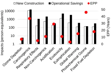
Figure 5. Base case environmental payback periods, normalized impacts from initial construction, and normalized 50 year cumulative impact savings. Photochemical ozone formation has the longest EPP of 50 years, while eutrophication has the shortest at 7 years. Cumulative impact savings, plotted on a log scale, span orders of magnitude with ozone depletion as the smallest and carcinogenics as the largest. The pairing of EPP and normalized impacts highlights the lack of correlation between impact magnitude and payback.
In Figure 5, instances where operational savings exceed initial construction impacts are
indicative of an EPP of 50 years or less. Pairing EPP with normalized impacts highlights the
lack of correlation between impact magnitude and payback. Eutrophication has the shortest
EPP and third greatest impact savings, indicating it is highly advantageous to undertake the
replacement project for this impact. Conversely, photochemical ozone has the longest payback
period and only modest impact savings, indicating that it is among the least beneficial. Ozone
depletion, with a short payback and small impact savings, would provide less motivation for
undertaking a replacement project.
These results also highlight the contrast between climate and toxicity impacts. Global
warming potential is a category often associated with green building projects and it has a
0
10
20
30
40
50
1
10
100
1000
10000
E
P
P
(Y
e
a
rs)
Im
p
a
cts
(pe
rson
-e
q
u
iv
a
len
ts)
26
moderate payback of 19 years, supporting its use in this application as it makes the project
appear advantageous. However, the 50 year cumulative savings are modest, 360 PEs, or
approximately 7 per year. At the same time, carcinogenic impacts have a payback of over twice
as long at 41 years, indicating a lesser advantage to building replacement, while the normalized
cumulative savings exceed 10,000 PEs. Ecotoxicity also exhibits a high quantity of impact
savings. While human health impacts, including carcincogenics, non-carcinogenics, and
respiratory effects, are more uncertain and not typically addressed in green building
assessment, Figure 5 indicates that they are non-negligible.
3.2
Energy Reduction
27
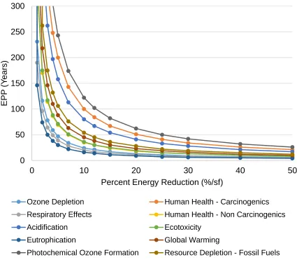
Figure 6. Percent energy reduction versus environmental payback period for TRACI impact categories. Increases in the annual percent energy reduction in the new versus existing building produce non-linear decreases in EPP.
Given that electricity is assumed to be used exclusively in both the existing and new
buildings, no paybacks are obtained at a 0% energy reduction since the new building introduces
new impacts through construction and does not have a mechanism for operational impact
savings. The relationship between percent energy reduction and EPP is not linear; as energy
reduction increases, there is incrementally less benefit per unit energy reduction. However, the
sensitivity to energy reduction varies by impact category; photochemical ozone formation and
carcinogenic impacts are more sensitive to the change, while respiratory effects and
eutrophication experience less change. A 15% decrease in energy consumption between the
0
50
100
150
200
250
300
0
10
20
30
40
50
E
P
P
(Y
e
a
rs)
Percent Energy Reduction (%/sf)
Ozone Depletion Human Health - Carcinogenics
Respiratory Effects Human Health - Non Carcinogenics
Acidification Ecotoxicity
Eutrophication Global Warming
28
old and new buildings reduces EPP for all impact categories except photochemical ozone
formation to within a projected building lifetime of 80 years. However it takes a 50% energy
reduction to reduce EPP to a more near-term timeframe of under 30 years across all impact
categories. These results indicate that energy reductions achieved by buildings in previous
studies can produce increased environmental performance as represented by shorter EPPs
across all impact categories.
3.3
Discount Rate
29
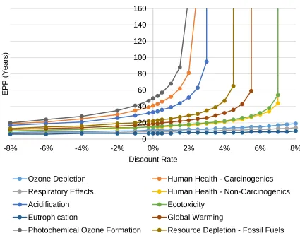
Figure 7. Percent discount rate versus environmental payback period for TRACI impact categories. Increases in discount rate produce non-linear increases in EPP. At an 8% discount rate, the highest rate considered, only ozone depletion, respiratory effects, and eutrophication all have finite discount rates under 20 years.
Figure 7 also illustrates that negative discount rates further improve EPP, though the
improvement is modest for all impact categories over a wide range of negative rates. If future
impacts are valued less than impacts today, represented with a positive discount rate, the annual
impact savings decrease, which increases the amount of time it takes to pay back impacts. As
discount rate approaches a market rate, it becomes less likely that a decision maker would opt
for building replacement. However, if future impacts are valued more than impacts today,
represented with negative discount rates, then those savings increase over time, shortening
payback.
0 20 40 60 80 100 120 140 160
-8% -6% -4% -2% 0% 2% 4% 6% 8%
E
P
P
(
Y
ea
rs)
Discount Rate
Ozone Depletion Human Health - Carcinogenics
Respiratory Effects Human Health - Non-Carcinogenics
Acidification Ecotoxicity
Eutrophication Global Warming
30
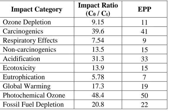
A determining factor in sensitivity to discount rate for an impact category is the ratio of
initial impacts to operational impact savings resulting from a more efficient new building. This
is reflective of the mathematical relationship contained within Equation 2 between C
0and C
t,
where C
0is initial impacts, and C
tis annual impact savings.
This ratio is increased by increasing initial impacts or decreasing annual impact savings.
Conversely, it is decreased by decreasing initial impacts or increasing annual impact savings.
This means that short EPPs are the result of either low initial impacts, high operational savings,
or a combination of the two for a particular impact category. Thus, EPP can be influenced by
all building life cycle stages, and designers have the option to either target initial or operational
impacts if trying to reduce EPP. Table 2 includes the impact ratios and EPPs for the base
scenario.
Table 2. Impact ratios for 25% energy reduction and 0% discount rate
Impact Category
Impact Ratio
(C
0/ C
t)
EPP
Ozone Depletion
9.15
11
Carcinogenics
39.6
41
Respiratory Effects
7.54
9
Non-carcinogenics
13.5
15
Acidification
31.3
33
Ecotoxicity
13.9
15
Eutrophication
5.78
7
Global Warming
17.3
19
Photochemical Ozone
48.4
50
Fossil Fuel Depletion
20.8
22
31
sensitive impact categories include eutrophication, respiratory effects, non-carcinogenics, and
ecotoxicity. These results further illustrate the significant differences in impact across different
impact categories.
3.4
Interaction of Energy Reduction and Discount Rate
32
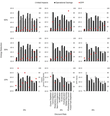
Figure 8. Environmental payback period and normalized 50 year cumulative impact savings when percent energy reduction and discount rate are varied simultaneously. EPP is represented on the left axis and normalized impacts on the right. The absence of a red circle for an impact category indicates there is not a payback under the specified conditions. Low discount rates and high energy reduction produce outcomes in which all impact categories pay back. Category labels shown in the bottom center figure apply to all figures.
Lower discount rates and higher energy reductions produce more optimal EPP scenarios.
In the cases shown, all impacts have paybacks for the 0% discount rate column with the
exception of photochemical ozone formation with 10% energy reduction, while 3 to 10
0 20 40 60 80 100 1E+0 1E+1 1E+2 1E+3 1E+4 1E+5
Initial Impacts Operational Savings EPP
0 20 40 60 80 100 1E+0 1E+1 1E+2 1E+3 1E+4 1E+5 0 20 40 60 80 100 1E+0 1E+1 1E+2 1E+3 1E+4 1E+5 0 20 40 60 80 100 1E+0 1E+1 1E+2 1E+3 1E+4 1E+5 0 20 40 60 80 100 1E+0 1E+1 1E+2 1E+3 1E+4 1E+5 0 20 40 60 80 100 1E+0 1E+1 1E+2 1E+3 1E+4 1E+5 0 20 40 60 80 100 1E+0 1E+1 1E+2 1E+3 1E+4 1E+5 0 20 40 60 80 100 1E+0 1E+1 1E+2 1E+3 1E+4 1E+5 Ozon e De pletion C ar ci no genics R es pira to ry Ef fec ts N on-Ca rcinog enics Acid ification Eco to xicit y Eut rophic ation Glo bal W ar m in g Phot oche mica l Ozo ne Foss il F uel D epletion EP P (Y ears) Impac ts (per s on -equi v al ents ) 0 20 40 60 80 100 1E+0 1E+1 1E+2 1E+3 1E+4 1E+5 50% 30% 10%
0% 4% 8%
Energy
Re
duc
tion
33
categories do not recognize paybacks in the 8% discount rate column. This illustrates that the
less a decision maker values future impacts, the better performing the new building must be to
recognize paybacks. Figure 8 also illustrates the decrease in cumulative impact savings as
percent energy reduction decreases and discount rate increases.
3.5
Variation in Material Selection
Preliminary analysis on the effect of different building materials on environmental impact
produced seven materials for further investigation: aluminum, glass, concrete, steel, iron,
copper, and terrazzo (composite flooring material). These materials are individually decreased
by 25% in OpenLCA and the percent decrease in EPP in each case is calculated and included
in Table 3. Shaded cells highlight instances of EPP decrease as a result of material decrease.
Table 3. Percent change in EPP due to 25% decrease in material input
Impact
Category
Aluminum
Glass
Concrete
Steel
Iron
Copper Terazzo
Ozone
Depletion
18%
9%
9%
9%
9%
0%
0%
Carcinogenics
15%
0%
0%
7%
0%
0%
0%
Respiratory
Effects
11%
0%
0%
0%
0%
0%
0%
Non-Carcinogenics
13%
0%
0%
7%
0%
7%
0%
Acidification
15%
3%
3%
3%
3%
0%
3%
Ecotoxicity
7%
0%
0%
0%
0%
0%
0%
Eutrophication
14%
0%
0%
0%
0%
0%
0%
Global
Warming
16%
0%
0%
0%
5%
0%
0%
Photochemical
Ozone
14%
2%
2%
2%
4%
0%
2%
Fossil Fuel
34
Each of the assessed materials are present in different quantities in the building, some
representing larger fractions of total weight or volume of the building than others. Additionally,
25% reductions in any given material would likely be hard to achieve, so these values are
meant to be representative of the relative impacts by material.
Large changes in material produce only modest changes in EPP, implying material
selection is not a primary factor for determining EPP. All material reductions of 25% produced
EPP reductions of less than 25%. The effect of each material on the overall building varies by
material. Decreasing aluminum results in a decreased EPP across all impact categories, steel
decreases 5 impact categories, and iron decreases 4 categories, while other materials affect 3
or less. Similarly, some impact categories are affected more than others. Ozone depletion is
affected by 5 of 7 materials examined, with a 9% or more decrease in EPP. Acidification and
photochemical ozone formation were both affected by 6 of 7 materials, though with more
modest EPP decreases.
The impact of aluminum is attributed to the environmental burdens associated with bauxite
mining, alumina production, and processing of alumina to aluminum. These refining, smelting,
and casting processes are each energy intensive and waste producing. For example, one ton of
alumina production creates as much as two tons of “red mud”, a toxic byproduct (Tan & Khoo,
2005). Thus, decreasing the quantity of aluminum in the building significantly decreases the
associated impacts.
3.6
Variation in Electricity Supply
35
amount of savings achieved by operating a new building. Thus, an EPP based on the current
grid mix is shorter than one based on the anticipated future grid mix, as illustrated in Figure 9.
Figure 9. Effect of grid transition over time on environmental payback period. As the electric grid becomes cleaner, EPP increases due to decreased impact savings between the existing and new building. Note that the grid mix is assumed to remain constant at the AEO 2016 value, while the other two scenario assume a changing grid mix over time based on the AEO Reference and Clean Power Plan (CPP) scenarios. The AEO 2016 mix is the same as the manual SERC mix contained in Table 1.
Transition to the 2050 AEO Reference Case mix from the 2016 AEO values produces a
EPPs of 100 to 125% of the base value depending on impact category. Similarly, a transition
to the 2050 AEO Reference Case with CPP, a scenario with larger renewables deployment,
leads to EPPs of 100 – 137% of the base value. It should be noted that the model produces EPP
at the resolution of one year, so it is possible that impact categories that did not experience a
change in EPP due to fuel supply changes may actually change slightly, but not enough to be
reflected in the model output. This is confirmed via graphical interpretation of the EPP results.
A similar trend is observed for the application of solar to both buildings as illustrated in
Figure 10. The 100% solar scenario applied to both buildings increases EPP to an average of
0
20
40
60
80
100
120
140
160
E
P
P
(Y
e
a
rs)
36
over 8 times longer compared to using the AEO 2016 scenario. However, the opposite is
observed for changes that are applied to the new building only. If only the new building
receives electricity via solar, EPP drops to an average of 40% of the AEO 2016 scenario.
Figure 10. Effect of 100% solar electricity supply on environmental payback period when applied to just the new building (green bars) and to both buildings (dark blue bars). EPP is plotted on a log scale. Application of solar to the new building only reduces EPP, while application to both buildings increases EPP.
Thus, all electricity supply changes are not created equal with respect to EPP. It is
important to consider the differences between improvements to the new building, such as
distributed renewable generation, and grid level improvements. Energy efficiency is found to
be less valuable on a cleaner grid, though this effect is magnified by the consideration of
electric-only buildings. The inclusion of fuel oil or natural gas heating would dampen the
response.
1
10
100
1000
E
P
P
(Y
e
a
rs)
37
3.7
Building Efficiency
Annual changes in energy usage are varied to determine the percent annual energy
reduction in the existing building or annual energy increase in the new building that would
eliminate EPP for different impact categories, meaning there is no longer a payback. Figure 11
illustrates the wide range of change required to elicit EPP elimination for different impact
categories in the 25% energy reduction, 0% discount rate scenario.
Figure 11. Comparison of changes to energy efficiency required to eliminate payback for specified impact categories, assuming 0% discount rate and an initial energy reduction of 25% between buildings. Impact categories with smaller allowable changes must operate closer to the designed and anticipated performance to maintain payback, whereas larger changes indicate payback is less sensitive to changes in annual energy use.