Using Multi-Class Classification Methods to
Predict Baseball Pitch Types
G
LENNS
IDLE, H
IENT
RAN Department of Applied MathematicsNorth Carolina State University
2108 SAS Hall, Box 8205
Raleigh, NC 27695
(919) 515-2382
Abstract
Since the introduction of PITCHf/x in 2006, there has been a plethora of data available for anyone who wants to access to the minute details of every baseball pitch thrown over the past nine seasons. Everything from the initial velocity and release point to the break angle and strike zone placement is tracked, recorded, and used to classify the pitch according to an algorithm developed by MLB Advanced Media (MLBAM). Given these classifications, we developed a model that would predict the next type of pitch thrown by a given pitcher, using only data that would be available before he even stepped to the mound. We used data from three recent MLB seasons (2013-2015) to compare individual pitcher predictions based on multi-class linear discriminant analysis, support vector machines, and classification trees to lead to the development of a real-time, live-game predictor. Using training data from the 2013, 2014, and part of the 2015 season, our best method achieved a mean out-of-sample predictive accuracy of 66.62%, and a real-time success rate of over 60%.
1
Introduction
Ever since Bill James published his work on sabermetrics four decades ago, Major League Baseball (MLB) has been on the forefront of sports analytics. While the massive amount of statistical data is generally used to examine historical player performance on the field in an effort to make coaching and personnel decisions, there is great potential for predictive models that has largely gone unnoticed. The implementation of the PITCHf/x system and distribution of large amount of pitching data publicly over the internet has sparked the use of machine learning methods for prediction, not just analysis.
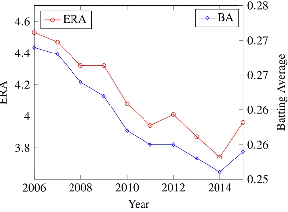
As shown in Figure1, pitchers have been getting better and better at preventing hits, lowering the average ERA and batting average across the league. While hitting a major league pitch will always be an incredibly difficult task, in this work we hypothesize that knowing what type of pitch is coming next may help the batter decide to swing or not and work to get him on base. In this paper, we compare three different machine learning techniques and their predictive abilities, seeking to find what feature inputs are the most informative and to develop a blind prediction in an attempt to anticipate the next pitch type. By comparing different techniques, we were able to find which would work best in a live game environment, attempting to predict the next type of pitch as before it would be thrown.
1.1
Literature Review
Previous research has mostly focused on a binary prediction, commonly a fastball vs. non-fastball split. This prediction has resulted in accuracy around 70% (Ganeshapillai and Guttag, 2012), with varying degrees of success for individual pitchers and different methods. This binary classification using support vector machines was expanded upon using dynamic feature selection in (Hoang, 2015), improving the results by approximately 8 percent. Because many classification methods were originally designed for binary classification, this prediction method makes sense, but we wish to expand it further into predicting multiple pitch types.
2
Methods
2.1
Data
The introduction of PITCHf/x was a revolutionary development in baseball data collection. Cam-eras, installed in all 30 MLB stadiums, record the speed and location of each pitch at 60 Hz, and data is made available to the public through a variety of online resources. MLB Advanced Media uses a neural-network based algorithm to classify those pitches, giving a confidence in the clas-sification along with the type of pitch (Fast, 2010). This information is added to the PITCHf/x database, along with the measure characteristics of the pitch and details about the game situa-tion. Using the pitch data provided at gd2.mlb.com, we were able to retrieve every pitch from the 2013, 2014, and 2015 seasons. Using 22 features from each pitch, we created data sets for every individual pitcher, adding up to 81 additional features to each data set, depending on how many types of pitches the individual threw. Here we consider seven pitch categories (with given integer values), fastball (FF, 1), cutter (CT, 2), sinker (SI, 3), slider (SL, 4), curveball (CU, 5), changeup (CH, 6), and knuckleball (KN, 7), and those that had a type confidence (the MLBAM algorithm’s confidence that its classification is correct) greater than 80%.
We restricted our data set only to pitchers who threw at least 500 pitches in both the 2014 and 2015 seasons, which left us with 287 total unique pitchers, 150 starters and 137 relievers as designated by ESPN. The average size of the data set for each pitcher was 4,682 pitches, with the largest 10,343 pitches and the smallest 1,108 pitches. Because each pitcher threw a different number of unique pitch types, not all the datasets are the same size. At the most, a pitcher could have 103 features associated with each pitch and at the minimum he could have 63. The average pitcher had 81 features.
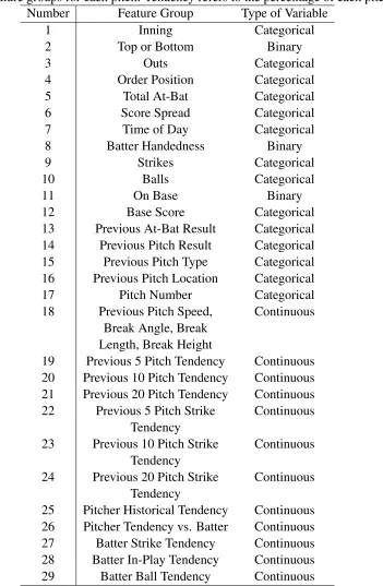
Table1gives a list of the features used, both those that can be taken from the immediate game situation and the features we generated using the historical data on for both pitcher and batter. Because of the size of the feature set, similar features are grouped together in the table, i.e. group 16 contains the previous pitch’s type, result, break angle, break length, break height, and the zone where it crossed the plate. Groups 19-26 have variable sizes due to the number of types of pitches each pitcher throws. Groups 27-29 are unique for each batter, containing the percent of each type of pitch he puts in play, has a strike on, or takes a ball on.
2.2
Model Development
2.3
Linear Discriminant Analysis
Linear Discriminant Analysis (LDA) is a method descended from R.A. Fisher’s linear discriminant he first introduced in (Fisher, 1936). Assuming two classes of observations have respective mean covariance pairs(~µ0,Σ0)and(~µ1,Σ1), then the linear combinations~w·~xhave the mean covariance pairs(~w·~µi, ~wTΣi~w)for i=0,1. Fisher determined the separation between the two distributions
(and therefore classes) as the ratio of the variance between the two classes to the variance within each class, i.e.
S= σ
2 between σwithin2 =
(~w·~µ1−~w·~µ0)2
~
wTΣ
1~w+~wTΣ0~w
= (~w·(~µ1−~µ0))
2
~wT(Σ
0+Σ1)~w
,
where the maximum separation between the classes is found when~w∝(Σ0+Σ1)−1(~µ1−~µ0). To go from the linear discriminant to LDA, we use the assumption that the class covariances are the same, i.e.Σ0=Σ1=Σ, then the proportional equation leads to~w·~x>c, where
~
w=Σ−1(~µ1−~µ0) c=1
2(~µ
T
1Σ−1~µ1−~µ0TΣ−1~µ0)
and so the decision of which class~x belongs to depends on whether the linear combination sat-isfies the inequality. In order to extend LDA to multi-class classification, the same assumption is made that each ofN classes has a unique mean~µi but the same covarianceΣ. The between class
covariance is found by
Σb=
1 N
N
∑
i=1
(~µi−~µ)(~µi−~µ)T,
where~µ is the mean of the means, and then class separation is determined by
S= ~w
T
Σb~w ~wTΣ~w .
We use a regularization parameter to shrink the covariance matrix closer to the average eigen-value of Σ. In the MATLAB implementation of LDA,N(N−1)/2 separations are made, making it comparable to the one-vs-one (OvO) technique for support vector machines. The final class decision is made by minimizing the sum of the misclassification error (MathWorks, 2016b).
2.4
Multi-class Support Vector Machines
createsNSVMs, and places the unknown value in whatever class has the largest decision function value.
For our model, we used the one-vs-one (OVO) method, which createsN(N−1)/2 SVMs for classification. For a set of p training data, (x1,y1), . . . ,(xp,yp) where xl ∈ Rn,l =1, . . . ,p and yl∈ {1, . . . ,N}is the class label forxl, then the SVM trained on theith and jth classes solves
min
wi j,bi j,ξi j 1 2(w
i j)Twi j+C
∑
`
ξ`i j
where(wi j)Tφ(x`) +bi j≥1−ξ`i j ify`=i,
or(wi j)Tφ(x`) +bi j≤ −1+ξ`i j ify`= j,
ξ`i j≥0.
where φ(x) =eγ||xi−xj|| is the radial basis function used to map the training data x
i,j to a higher
dimensional space and C is the penalty parameter. After all comparisons have been done, the unknown value is classified according to whichever class has the most votes from the assembled SVMs.
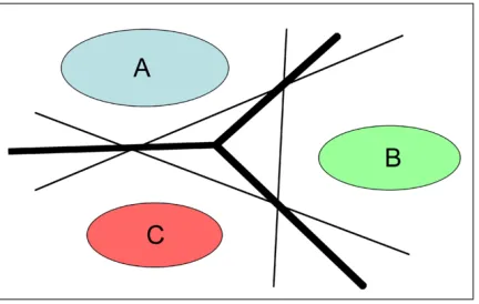
Figure2shows a basic representation of the differences between the OVA and OVO methods. The middle triangle formed by the OVA method leaves a gap where the classification algorithm can fail to place an unknown value, but since the OVO method does not have any blind spots, we used it for our classification. We used a modified grid search (Finkel, 2003) to optimize for both parametersC and γ, using the five-fold cross-validation accuracy of the training set to find the optimal parameters.
2.5
Classification Trees
In order to compare our results to (Woodward, 2014), we also implemented classification trees, using random forests. We used the MATLABCART (Classification And Regression Trees) imple-mentation that creates aggregate random forests of trees, known as TreeBagger.
Classification Trees are a specific type of binary decision tree that give a categorical classifica-tion as an output. The input set is used in the nodes of the tree, determining which feature to split at each node and what criterion to base that decision on. To determine node impurity, MATLAB classification trees use the Gini diversity index (gdi), given byI=1−∑Ni=1p2(i), whereN is the number of classes andp(i)is the fraction of each classithat reaches the node. The gdi is a measure of the expected error rate at the node if the class is randomly selected according to the distribution of the classes at that node.
process is repeated until the total impurity is minimized and the end leaf nodes are found. To combat overfitting, however, classification trees are pruned by merging leaves that have the most common class per leaf (MathWorks, 2016a).
3
Results
3.1
Overall Prediction Accuracy
To establish a value for comparison, we found the best ”naive” guess accuracy, similar to that used in Ganeshapillai and Guttag (2012). We define this naive best guess to be the percent of time each pitcher throws his preferred pitch from the training set in the testing set. Consider some pitcher who throws pitch types 1, 2, 4, and 5 with distributionP={p1,p2,p4,p5}where∑pi=1, and his
preferred training set pitch is max(Ptrain) =p2, then the naive guess for the pitcher isPtest(p2). For example, since Jake Arrieta threw his sinker the most in the training set (26.31%), we would take the naive guess as the percentage of the time he threw a sinker in the testing set, which gives a naive guess of 34.03%. For the random forest method, we predicted 48.33% of his pitches correctly, so we beat the naive guess by 14.30% in his case. For all 287 pitchers, the naive guess was 54.38%.
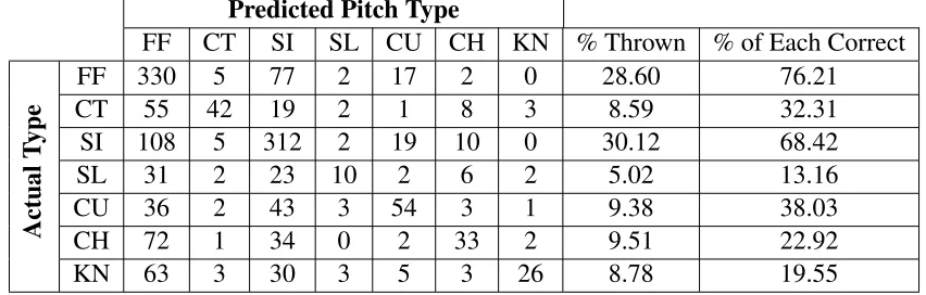
Table 2shows a breakdown of each type of pitch predicted for Odrisamer Despaigne by the random forest method, as well as the accuracy for each specific pitch, showing that for each pitch type, the accuracy of the model prediction improves the naive guess. We take this style of compar-ison from (Woodward, 2014), who gives an outline of a decision tree based prediction model, but does not go into detail or use more than a handful of examples, so we cannot fully compare to his results.
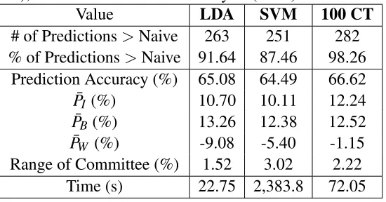
Table3shows the prediction results from each individual method. On average accuracy alone, Classification Trees had the best prediction accuracy of 66.62%. The number of pitchers we pre-dicted better than naive is given, as well as the percentage of the 287 total pitchers that number represents. The average prediction accuracy is shown, given along with the overall average im-provement over the naive guess, denoted ¯PI, the average improvement for those pitchers who did beat the naive guess, denoted as ¯PB, and the average amount the pitchers who did not beat the naive guess failed by, denoted by ¯PW. Given the number of pitchersN with respective prediction value
worse than the naive guessNW, we find
¯ PI =
N
∑
i
Pi−Gi
N
¯ PB=
NB ∑
i
Pi−Gi
NB
¯ PW =
NW ∑
i
Pi−Gi
NW .
We also give the average range of accuracy between the most and least accurate members of each committee as well as the average time for each pitcher’s model to be trained and tested. As shown in Table3, the random forests of classification trees outperformed both LDA and SVM by a wide margin. Basing the judgement solely on how many pitchers were predicted better, the random forests were near-perfect, leading the average prediction accuracy and improvement to also be higher. LDA outperforms the random forests only when we examine the average improvement for those pitchers who we are able to beat the naive guess for, but conversely also has much worse performance for the pitchers we do not beat the naive guess for. At this stage, we undertook further comparative analysis to determine if the random forests were the best method overall.
3.2
Prediction by Count
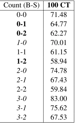
A common analysis in any pitch prediction is breaking down prediction success rate by each pitch count. There are twelve possible counts for any at-bat, three where the batter and pitcher are even, three where the pitcher is ahead in the count (more strikes than balls), and six where the batter is ahead (more balls than strikes). Similar to other works, On the very batter-favored count of 3-0, we were able to predict 104 pitchers (36.24% of 287 pitchers) totally correct, i.e. for every pitch they threw on a 3-0 count, we predicted them all exactly. The total counts and average success rates for the random forest classification tree method are given in Table4. Pitcher ahead counts are bolded, batter-favored counts are italicized.
The high success rate on counts in which the batter is ahead is not surprising, given that a pitcher is more likely to throw a controllable pitch in order to even the count or to avoid a walk. Batter-behind counts give the pitcher much more freedom, which explains the lower average pre-dictability.
3.3
Comparison with Standard Statistics
improvement over the naive guess to the pitchers’ wins-above-replacement (WAR) and fielding-independent-pitching (FIP) statistics. FIP is an extension of a pitchers’ earned run average (ERA) that examines only outcomes over which the pitcher had control. The comparisons are shown below in Table5.
We looked at those pitchers who improved over the naive guess the most rather than just the pitchers with the highest overall prediction accuracy because some pitchers highly favor one type of pitch, sometimes throwing it upwards of 90% of the time, and so even with only a small im-provement they would be one of the highest predicted pitchers.
After examining the standard metrics next to the prediction improvement, we found a small correlation between the ability of the classification trees to improve on the naive guess and the overall pitcher performance. On average, the pitchers who were hardest to beat the guess had a WAR almost 0.5 higher than those who were most improved on and around 0.2 less FIP. While not a huge difference in performance metrics, these results suggest that the harder it is to predict a pitcher, the better he is in a game. We also examined the number of pitch types a pitcher throws, and we find that on average, those pitchers harder to improve prediction wise, who had higher average WAR, throw fewer unique pitch types. This may suggest that these pitchers have high prediction levels already due to an over-reliance on a single pitch and a lack of diversity, leading to a high naive guess.
4
Variable Importance
Post-processing techniques can be used to determine what features are the most important in a model, so we used the models created for the results previously discussed to find measures of vari-able importance with the permuted varivari-able delta error (PVDE) for the random forests of classifi-cation trees. The PVDE is found during the construction of each random forest for each variable by first finding the expected error (EOi) against a hold-out validation set, similar to the cross-validation used for the parameter optimization. The values for a particular variablexiare then randomly
per-muted across every observation in the subset of the training data used for the tree construction, and the expected error value (EPi) is found against the same holdout set.
5
Live Pitch Prediction
At the start of this research, one of the reasons we examined different machine learning methods of prediction was to determine what would work best in real time in a live game environment. The previous experiments were all done in a ”bulk” setting, i.e. predicting all of the testing set all at once. While this gives a way to measure the effectiveness of each method, the construction of the testing datasets was not reflective of the way a dataset would be built during an actual baseball season. Any live prediction training set could only be updated with after each game, and would only show historical pitcher or batter tendencies up to the day before a game was played.
The data for the live predictions was parsed appropriately, creating pitcher preferences and batter performance measures up until the day being predicted. We examined the games in the regular season of September and October 2016, creating models for each pitcher for not only predicting the type of pitch thrown, but also the speed of the pitch and the location of the pitch (as determined by the zones detailed in Chapter 2). Models were created for every pitcher who pitched in September and October, as long as he had pitched at some point after the All-Star break (mid-July) and before September 1st. There was a large amount of data available to test on, and the characteristics of the data are shown in Table7.
While the overall prediction accuracy for all the pitches thrown was 59.07%, the average accu-racy across each pitcher in each game was 60.69%
6
Conclusion and Future Work
Because (Bock, 2015) and (Woodward, 2014) are the only examples of multi-class pitch prediction we have found, they are the standard for comparison. An example of pitch prediction using Markov Chains was done by (Malter, 2016), but it is not a situational-based model. Our model takes data that is available in the moments before the next pitch is thrown and gives the batter and manager better knowledge of what is coming than he would have had beforehand. Our results are better than any other purely predictive model of a multi-class pitch type thus far.
Moving forward, we plan to employ a feature selection method similar to one used in (Hoang, 2015) to find which inputs are the most important to the prediction, or even if reducing the size of the feature vectors may improve the prediction, as we may work to avoid the curse of dimension-ality. Due to the construction of the multi-class problem, implementing pre-processing techniques such as F-score or ROC curve analysis may require the introduction of classification using a Di-rected Acyclic Graph. Using these pre-processing techniques along with the information learned from the variable importance may help improve the live pitch predictors as well.
References
Joel R. Bock. Pitch Sequence Complexity and Long-Term Pitcher Performance. Sports, pages 40–55, March 2015.
Mike Fast. The Internet cried a little when you wrote that on it. The Hardball Times, 2010.
Daniel Finkel. DIRECT Optimization Algorithm User Guide. Center for Research in Scientific Computation, NCSU, 2003.
R.A. Fisher. The use of multiple measurements in taxonomic problems. Annals of Eugenics, 2: 179–188, 1936.
Gartheeban Ganeshapillai and John Guttag. Predicting the Next Pitch. Proceedings of the MIT Sloan Sports Analytics Conference, 2012.
Phuong Hoang. Supervised Learning in Baseball Pitch Prediction and Hepatitis C Diagnosis. NC State University, Ph.D. Thesis, 2015.
Danny Malter. Using Markov Chains to Predict Pitches, 2016. URL http://danmalter. github.io/r/2016/03/28/Markov-chains.html.
MathWorks. fitctree.m documentation, 2016a. URL http://www.mathworks.com/help/ stats/fitctree.html.
MathWorks. Discriminant Analysis, 2016b. URL http://www.mathworks.com/help/stats/ discriminant-analysis.html.
Table 1: Feature groups for each pitch. Tendency refers to the percentage of each pitch type. Number Feature Group Type of Variable
1 Inning Categorical
2 Top or Bottom Binary
3 Outs Categorical
4 Order Position Categorical
5 Total At-Bat Categorical
6 Score Spread Categorical
7 Time of Day Categorical
8 Batter Handedness Binary
9 Strikes Categorical
10 Balls Categorical
11 On Base Binary
12 Base Score Categorical
13 Previous At-Bat Result Categorical 14 Previous Pitch Result Categorical 15 Previous Pitch Type Categorical 16 Previous Pitch Location Categorical
17 Pitch Number Categorical
18 Previous Pitch Speed, Break Angle, Break Length, Break Height
Continuous
19 Previous 5 Pitch Tendency Continuous 20 Previous 10 Pitch Tendency Continuous 21 Previous 20 Pitch Tendency Continuous 22 Previous 5 Pitch Strike
Tendency
Continuous
23 Previous 10 Pitch Strike Tendency
Continuous
24 Previous 20 Pitch Strike Tendency
Continuous
Table 2: 100 CT pitch-specific model predictions for Odrisamer Despaigne, overall accuracy 53.30%.
Predicted Pitch Type
FF CT SI SL CU CH KN % Thrown % of Each Correct
Actual
T
ype
FF 330 5 77 2 17 2 0 28.60 76.21
CT 55 42 19 2 1 8 3 8.59 32.31
SI 108 5 312 2 19 10 0 30.12 68.42
SL 31 2 23 10 2 6 2 5.02 13.16
CU 36 2 43 3 54 3 1 9.38 38.03
CH 72 1 34 0 2 33 2 9.51 22.92
Table 3: Average values to compare support vector machines (SVM), random forests of 100 clas-sification trees (100 CT), and linear discriminant analysis (LDA).
Value LDA SVM 100 CT
# of Predictions>Naive 263 251 282 % of Predictions>Naive 91.64 87.46 98.26
Prediction Accuracy (%) 65.08 64.49 66.62 ¯
PI (%) 10.70 10.11 12.24 ¯
PB (%) 13.26 12.38 12.52
¯
PW (%) -9.08 -5.40 -1.15
Table 4: Average Prediction accuracy for each pitch count for the Classification Tree method. Pitcher favored counts are shown in bold, batter-favored counts in italics.
Count (B-S) 100 CT
0-0 71.48
0-1 64.77
0-2 62.27
1-0 70.01
1-1 61.15
1-2 58.94
2-0 74.78
2-1 67.43
2-2 59.84
3-0 83.00
3-1 75.62
Table 5: Random Forest Classification Tree Prediction Improvement Compared to Number of Pitch Types Thrown (PTT), FIP, and WAR.
Most Improved Least Improved
Pitcher PTT % Imp. FIP WAR Pitcher PTT % Imp. FIP WAR
J. Johnson 4 79.45 3.73 0.56 M. Estrada 4 -1.74 4.40 3.60 T. McFarland 4 72.84 4.47 -0.30 J. Lyles 5 -1.37 3.79 0.30 L. Avilan 5 70.24 3.66 0.29 J. Hughes 3 -1.30 3.81 1.20 J. Hahn 5 67.84 3.51 1.00 J. Odorizzi 4 -1.26 3.61 3.60 H. Santiago 5 63.40 4.77 1.80 U. Jimenez 4 -0.09 4.01 2.60
J. Garcia 5 63.04 3.00 3.90 K. Uehara 2 0.00 2.44 1.30
J. Kelly 5 61.95 4.18 1.00 L. Lynn 5 0.43 3.44 3.50
K. Gibson 5 59.88 3.96 3.20 K. Gausman 5 0.50 4.10 1.30
T. Roark 5 58.06 4.70 0.70 J. McGee 2 0.52 2.33 1.00
Z. Britton 2 57.86 2.01 2.50 B. Colon 5 0.62 3.84 1.00
Table 6: Variable Importance for Permuted Variable Delta Error for all pitchers. 1 means highest importance, 29 means lowest importance.
Feature Group PVDE
Inning 16
Top or Bottom 29
Outs 27
Order Position 18
Total At-Bat 6
Score Spread 21
Time of Day 25
Batter Handedness 7
Strikes 2
Balls 3
On Base 28
Base Score 19
Previous At-Bat Result 24 Previous Pitch Result 10 Previous Pitch Type 4 Previous Pitch Location 8
Pitch Number 1
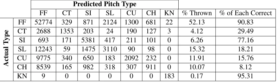
Table 7: Python live pitch predictions for September 1st through October 2nd, 2016, with overall accuracy 59.07%.
Predicted Pitch Type
FF CT SI SL CU CH KN % Thrown % of Each Correct
Actual
T
ype
FF 52774 329 871 2124 1300 681 22 52.13 90.83
CT 2688 1353 203 24 190 127 3 4.12 29.49
SI 693 171 5381 417 211 101 0 6.26 77.16
SL 12243 59 1475 3110 90 98 0 15.32 18.21
CU 9775 340 650 183 2092 232 0 11.91 15.76
CH 8539 165 982 318 307 911 0 10.07 8.12
2006 2008 2010 2012 2014 3.8
4 4.2 4.4 4.6
Year
ERA
ERA
0.25 0.26 0.26 0.27 0.27 0.28
Batting
A
v
erage
BA