THE SPATIAL DISTRIBUTION OF TRANSIENT ALLELES IN A SUBDIVIDED POPULATION: A SIMULATION STUDY

(1)

MONTGOMERY SLATKIN*

Department of Biophysics and Theoretical Biology, The University of Chicago, Chicago, Illinois 60637

A N D

DEBORAH CHARLESWORTH

School of Biological Sciences, The University of Sussex, Palmer, Brighton BNI 9QG, Sussex, United Kingdom

Manuscript received August 24, 1977 Revised copy received February 28, 1978

ABSTRACT

The spatial distributions of newly introducted alleles in a subdivided population are generated using a computer program to model the processes of selection, gene flow and genetic drift. Advantageous, neutral and deleterious alleles are considered, and certain aspects of the patterns generated by new alleles that are ultimately fixed and ultimately lost are examined. To characterize the spatial pattern of rare alleles, the distribution, Pi, the probability that the new allele is found in exactly i local populations before it is lost, is defined and estimated from the simulations. The shape of the Pi distribution is surprisingly similar for selected and neutral alleles. For advantageous alleles going to fixation, the ‘.wave of advance” is set up quickly, but stochastic effects reduce the wave speed from FISHER’S (1937) value. Gene flow is much more effective in dispersing alleles in a two-dimensional array than in one dimension. Long distance gene flow has a much smaller effect in two dimensions than in one dimension.

spatial patterns of alleles in a subdivided population have been used in a T z r i e t y of contexts to infer something about the relative importance of gene flow, natural selection and genetic drift in determining those patterns. HALDANE

(1948) and subsequent workers have used clinal patterns in allele frequencies to estimate the magnitudes of selection coefficients and dispersal rates. EHRLICH and RAVEN (1969) have used the frequent occurrence of genetic divergence of adjacent populations to argue that gene flow is an unimportant evolutionary process for many species. LEWONTIN and KRAKAUER (1973) have attempted to use the frequency distribution of F coefficients from isolated populations to assess the relative importance of genetic drift and selection. CHAKRABORTY and NEI (1974) have used the retardation of the rates of increase in the genetic distance between isolated populations as an estimate of the gene flow between those populations.

All of these uses of information about the genetic structure of subdivided populations are based on the implicit or explicit assumption that the populations have

* Permanent address: Department of Zoology, NJ-15, University of Washington, Seattle, Washington 98195.

(2)

794 M. SLATKIN A N D D. CHARLESWORTH

reached their equilibrium or asymptotic states. However, that may not be so because some populations may be newly founded, environmental conditions may have recently changed or new alleles may have recently entered the population by mutation or gene flow from an external source. These difficulties are well known, but these are good reasons for analyzing models of populations at or near equilibrium. There must be a clear understanding of the equilibrium or asymptotic properties of a model to provide a basis for understanding its complete, time dependent behavior. In addition, the structure of models of gene flow, selection and drift is generally so complex that there are only a few cases for which a complete nonequilibrium analysis can be carried out (e.g., NEI and FELDMAN 1972; LATTER 1973;

FLEMING

and Su 1974).

The purpose of this paper is to provide some information about the spatial patterns in the distribution of newly arising alleles in a subdivided population. This study is complementary to studies of equilibrium or asymptotic states. One approach to this problem is to find those results from models of a subdivided population that do not depend on the pattern of subdivision. MARUYAMA (1971b, 1974) has successfully taken this approach to show that for some selection models the probabilities of fixation, net heterozygosity and some other quantities are independent of the population structure. Our approach here is different in that we are trying to find those features of the results that do depend on the population structure. With this approach, it may be possible to obtain information about the interaction of gene flow with selection and genetic drift and to use that information to understand more about the genetic structure of natural populations. There are at least three questions that arise naturally in considering the spatial distribution of transient alleles: (1) For alleles that are ultimately lost, are there consistent differences between any features of the spatial patterns for advantageous, neutral and deleterious alleles? (2) For alleles that are ultimately fixed, are there differences between the transient patterns of advantageous and neutral alleles? (3) What are the effects of the dispersal patterns of a species on the spatial patterns of alleles that are both lost and fixed?

(3)

SPATIAL DISTRIBUTION O F T R A N S I E N T ALLELES 795

METHODS

We wrote a computer program to simulate the changes in the frequencies of two alleles a t a locus i n a diploid, monecious species distributed in n local populations. To simplify terminology, we will refer to each local population as a deme and to the set of n demes as the population. Each deme is assumed to be of the same size, N , and the fitnesses of the three genotypes are the same in all demes. Selection of adults, followed by random mating, takes place in each deme independently, and then gene flow takes place through the movement of juveniles before the next generation begins. All of our results are in terms of the state of the population after the gene flow stage.

The population is completely described by the genotype frequencies in each deme in each generation. The initial conditions for all of our runs were the same: all the demes were homozy- gous for one allele ( A ) , except one which had a single heterozygote ( A a ) . We will refer to the allele that is initially rare as the mutant allele, and the results will be described i n terms of its loss o r fixation.

The selection coefficients on the three genotypes AA, Aa, and aa were written as 1, 1

-

hs,

1 - s . The first step in each generation was the computation of the expected frequency of the mutant in an infinite pool of gametes formed after selection has already acted. Thus, if P is the frequency of A in the adults in a deme, then

P

-

P ( 1 - P ) 1 -2hhsp(l-p) -s(l--p)Z

p’

is the frequency of A in the gametes produced. The number, p’, is used to generate the genotypes of the individuals that remain in the population and to generate the genotypes of the immigrants.

Our procedure was first to compute the total number of immigrants to each deme, and then to c o m p t e the genotypes of the individuals descended from the nonmigrants. The geometric pattern of the demes was completely determined by the probabilities of exchange of migrants between every pair of demes. The migration process was assumed to be spatially homogeneous. We considered two types of models. The one- and two-dimensional stepping stone models were specified by the set mi, the migration rates between demes i steps apart. Demes a t or near the boundaries of the arrays exchanged fewer migrants because they had fewer demes within i steps. In all the results presented, n = 51 for the one-dimensional array, n = 100 for the two- dimensional array, and n = 50 for the island model. In the one- and two-dimensional models, the mutant was introduced in a central deme. The island model was described by a single parameter, m, the migration rate between a deme and a single other deme chosen at random. BY migration rate m between two demes, we mean that they exchange an average of mN individuals each generation.

For each pair of demes exchanging migrants, the total number of migrants was generated using a Poisson random number generator that produced a distribution of mean, N m , where m

is the appropriate rate. Then, the genotypes 3f the migrants from one deme to the other were found using the appropriate p’ and a second random number generator. The genotypes of all the immigrants to each deme were accumulated in a buffer. The genotypes of the offspring of the nonmigrants were then generated so that the total was again N . Thus, for example, if there were a total of six immigrants to a particular deme, the genotypes of N-6 individuals would be generated using a multinomial random number generator with the parameters P ’ ~ , 2p‘ ( I - p ‘ ) and (1-p’)2. Each replicate was run until the mutant was lost o r fixed.

(4)

796 M. SLATKIN A N D D. CHARLESWORTH

was checked by inspection of very detailed output to ensure that the distribution of numbers of migrant individuals agreed with a Poisson distribution, that the composition of the immigra- tion arrays was consistent with the gene frequencies employed, and that these arrays were correctly incorporated into the recipient populations.

RESULTS

The results will be presented in three parts corresponding to the three questions asked in the introduction. In the first two sections all the results are from simulations of a one-dimensional array with gene flow only between adjacent populations. In the third section, we consider the effect of changes in the migration pattern and changes in the geometric structure of the population.

(1) We consider separately the spatial pattern of mutants that will ultimately be lost from the population, because a large majority of them will be rare throughout the time they are present. While it is difficult in a particular species to estimate the frequencies of rare alleles, it may be easier to determine their presence or absence in a local population, I t may be possible to gain some information either about the selection coefficients affecting the rare alleles or something about the pattern of gene flow from such data. To do so, it would be necessary to know the expected pattern under different types of selection and gene flow.

From our simulation results, we can compute an estimate of the probability

Pi,

that, given that a mutant is found in the population but is ultimately lost, it is

found in exactly

i

demes. This estimate is found for each set of parameter values by accumulating, over all replicate runs, the total number of generations the mutant is in

i

demes. Some results are shown in Table 1. The same migration rate was used in all cases. For the neutral mutant, only

25

demes were used to reduce the running time to a reasonable level.

It is important to realize that the

Pi

found in this way differs from the probability that a new mutant will ever enter the total

i

demes. This latter probability, as considered by CRUMP and GILLESPIE (1976) for a neutral allele, does not take into account the fact that once a new mutant reaches a larger number of demes, it

is likely to be present in that number of demes for a much longer time than a mutant that is present in only a single deme. Thus, in computing only the probability that a mutant reaches

i

demes, the likelihood that such an allele would be observed would be greatly underestimated.

There seems to he no simple, one- or two-parameter family of probability distributions to which the computed

Pi

can be fitted. The values of PI are too large for an exponential o r negative binomial distribution, and, even excluding the first class, there is a significant deviation from an exponential fitted to the remaining

Pi. For the purposes here, it will be sufficient to use the mean value of

i, T

defined by

S = z i P ,

( 2 )

and P, to characterize

Pi.

(5)

TABLE I Pi, the probability that, if a mutant is observed in ihe population, it will be found in exactly i demes, and i, the mean of i for different selection regimes No. populations _____

1 2 3 4 5 6 7 8 9 ₁₀ ₁₁ ₁₂ ₁₃ ₁₄ ₁₅ ₁₆ ₁₇ ₁₈ ₁₉

20 21 22 23 24 25

hz0.5 h=0.5 s=O.O8 ~53.04 0.7125 0.6460 0.1881 0.1867 0.0766 0.0789 0.0202 0.0411 0.0048 0.0224 0.0002

0.0115 0.0070 0.0045 0.001

7

0.00~02

-__.__.

h=0.5 s=0.02 _0.5283 _0.1857 _0.1069 _0.0539 _0.0438 _0.0367 _0.0232 _0.0126 _0.01057 _0.0029 _0.0003

h=O s=O.Ol _0.4636 _0.1796 _0.0907 _0.0594 _0.0513 _0.014.28 _0.0372 _0.0239 _0.0115 _0.01

60

0.0128 0.0054 0.0053 0.0006

~-

h=0.5 s=O.Ol 0.3943 0.1638 0.1272 0.0979 0.0775 O.MO6 0.0293 0.0199 0.0171 0.0100 0.0076 0.0046 0.0003 0.0001 h=l s=O.Ol 0.3674 0.1604 0.1175 0.0773 0.0682 0.0562 0.0520 0.0461 0.0297 0.0175 0.0061 0.0015 0.0003

____

s=o

~- 0.2855 0.1198 0.0895 0.0680 0.0555 0.046'3 0.0416 0.0374 0.0317 0.0281 0.0277 08.0227 0'.0175 0.0152 0.0137 0.0154 0.08149 0.014'0 0.01

20

0.0088 0. 0013

9

08.080330 0.0033 0.01079

o.ai

62

h=l s=-0

01

0.2944 0.1152 0.0796 0.0721 0.0784 0.0693 0.06% 0.0545 0.0494 0.0394 0.0262 0.0128 0.0081 0.0103 0.0094 0.0086 0.005

1

0.0028 0.0018 0.0002 0.0001

--

h=0.5 s=-O.Ol

__._

0.5026 0.1737 0.1

114

0.0743 0.0513 0.0319 0.0210 0.01

84

0.0103 0.00135 0.0010 0.0004

h=O s=-o.

0

1

08.5447 0.1789 0.1031 0.0697 0.M9 0.0358 0.0149 0.0051 0.0010

--__

h=0.5 s=-O.OZ

k0.5

s=-0.04

s=-0.08

0.5668 0.1958 0.1018 0.0511 0.0372 0.0246 091

07

0.0039 0.0025 0.001

8

0.0016 0.00118 0.0003 0.6304 0.2118 0.0946 0.0367 0.01

70

0.0079 0.0015 0.0001

0.7389

%

0.1905 0.0581

4

0.0119

w

0.0006

r

H 4 4 F r M F m v1

(6)

798 M. SLATKIN A N D D. CHARLESWORTH

for h = 0.5 and s = 0.01 for two sets that are not shown in Table 1 of 865 and 994 replicates, i: was 2.59 and 2.46 and

P ,

was 0.5336 and 0.4979. For nine sets of

1000 replicates with s = 0, the values of

P,

ranged from 0.1810 to 0.3789, with

similar variation in

T.

The values in Table 1 f o r s = 0 are the average for the nine sets. In all sets of replicates,

Pi

decreased rapidly with

i

in the same manner as in Table 1

,

but the exact values depend strongly on the maximum number of demes entered. A mutant that enters several demes can be present in the population f o r hundreds or thousands of generations. Those events are rare, but extremely important, in determining the estimates of Pi.

The results in Table 1 are not very encouraging. The expected spatial patterns, as measured by

Pi,

of advantageous, neutral or selected alleles are similar enough that little could be learned from estimates of

Pi

for a particular collection of alleles that are rare and presumed to be in the process of being lost. But, in addition,

Pi depends strongly enough on the selection coefficients that it could not be used to estimate m, even if it were possible to assume such a simple population structure.

It

may be somewhat surprising that 5 decreases as the intensity of selection on both advantageous and deleterious mutants increases. The reason is slightly different for the two cases. For a deleterious mutant, stronger selection will cause the mutant not to reach as high a frequency in any deme, thus reducing its chances of being carried by a migrant. For an advantageous allele, stronger selection makes it more likely to go to fixation once it reaches an appreciable frequency in any deme. As the cases for different levels of dominance indicate, it is the selection on the heterozygotes that is most important.

Because of the character of the results in Table 1 and a comparison of the estimates of

Pi

for cases which differ only in the sign of s, it was suggested both by

J.

F.

CROW and one of the referees that, for a given h, the

Pi

depend only on the

magnitude of s, not on its sign. Such a result has been shown for sojourn times in a single panmictic population (MARUYAMA and KIMURA 1974), but the problem here is far more complex and a demonstration that the Pi be independent of the sign of s would involve an analysis of the multidimensional diffusion process for the frequencies of the alleles in all of the demes. Nevertheless, there is sufficient variability in the simulation results that this suggestion may be true and cannot be contradicted by the relatively small number of simulations that we could run.

From MARUYAMA’S (1971b) analytic theory, the probability of fixation of a neutral or semidominant allele in a subdivided population is the same as in a single panmictic population with the same total number of individuals as the subdivided population. An allele that is rare in a subdivided population will, with a high probability, be ultimately lost, even if it is found in several demes. How- ever, there is some chance that an allele can reach a high frequency in one or more demes before being lost. The pattern is similar for selected and neutral mutants. This is illustrated in Table 2, where the dependence of the maximum frequency in any deme of the mutant on the maximum number of demes it enters

(7)

TABLE 2 Maximum frequency of the mutant in any deme as a function of the maximum number of demes entered

9 =1

9 r

____ ______~~ ~______ ~_____ ~ Selection Maximum number of demes 17

...

36

2

0 Z 0 r

-- coefficient 1 2 3 I. 5 6 7 8 9 10 11 12 13 14 15 16 ___ ~~ - 0.01 0.07 0.17 0.22 0.29 0.38 0.39 0.66 0.41 0.62 0.77 0.00 0.11 0.25 0.40 0.25 0.60 0.57 0.66 1.0 0.91 1

.o

1 .o 0.00 0.11 0.18 0.24 0.24 0.48 0.44 0.53 0.70 0.56 0.71 0.76 0.95 0.99 1.0 -0.01 0.17 0.27 0.45 0.36 0.43 0.52 0.88 0.66 0.96 0.99 1.0

r

2

E

a one-dimensional array of demes with gene flow only between adjacent demes was used, and n = 51, N = 50, h = 0.5 and m = 0.02 were the

2

9

parameters

values.

r r M r M

(8)

800 M. SLATKIN A N D D. CHARLESWORTH

higher its frequency can be in any one of them. However, if the mutant is rare in the population as a whole, then it is still likely to be lost. In Table 2, the results of two sets of replicates for the J = 0 case are shown.

(2) The process of fixation offers somewhat more encouragement for distin- guishing different types of alleles, but there is still a considerable stochastic com- ponent to the process. For the parameter values we have used, the fixation of slightly deleterious alleles is so unlikely that it never happened during our simu-

lations. However, if a deleterious allele were fixed, the process would have to be dominated by genetic drift, so that it is reasonable to assume that the time course would be similar to that for the fixation of a neutral allele.

For an advantageous mutant, our simulations indicate that, if it is going to be fixed, then it will tend to increase in frequency in one or, at most, a few demes. Then, gene flow will tend to spread the allele to other demes. Therefore, the “wave of advance” described by FISHER (1937) tends to be set up relatively quickly, and a distinct cline is apparent not just as an asymptotic state, as in FISHER (1937)

,

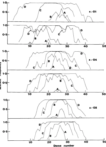
but throughout the spread of the allele. We can see this in several cases in Figure 1. The selection coefficients were chosen to range from relatively weak selection

( N s = 0.5) to somewhat stronger selection ( N s = 2,4). For each selection co-

efficient, the time course of the first two fixations is shown. This is preferable to plotting average values from several replicates because both the general pattern and the extent of the case to case variation can be illustrated. Even for weak selection, a cline is apparent throughout the fixation processes.

There is considerable variation among replicates, particularly in the initial stages. There is some delay before the mutant increases to a significant frequency in any deme and the magnitude of the delay differs from run to run. In Figure la, the maximum frequency after 200 generations is 0.71 while in Figure l b it is only

0.28. An even greater difference is found in Figures I C and Id. Also, the center from which the allele spreads may be different. In all cases the allele was introduced in deme 26 but in Figure lb, for example, the center is deme 19 or 20. The variability is accounted for by the fact that we have chosen a low rate of gene flow (2 Nm = 2) so that the stochastic effects due to the variance associated with the small number of migrants are important.

The fact that the cline tends to be set up quickly supports the results from the heuristic model in SLATKIN (1976), which shows that it is unlikely that gene flow will result in the movement of an allele from one population to another unless that allele has reached an appreciable frequency in the first population. By that time, selection would drive the advantage allele to fixation in the first deme before it increases significantly in the second. Expressing this in terms of time scales, the time scale associated with the increase in allele frequency due to selection is shorter than the time scale associated with the movement of the allele between populations because of gene flow.

We can also use the simulation results to estimate the speed of the advancing wave and compare it with the analytic values from the asymptotic theory of

(9)

SPATIAL DISTRIBUTION O F T R A N S I E N T ALLELES

1.0-

0 - 5

k

a

g

1-0-

C P)

U

w-

c

5

0 5 -

i

c

80 1

-

0

1 1.0-

0 - 5

-

I

10 2 0 3 0 4 0 5 0

Deme number

FIGURE 1.-Frequency of mutant us. deme number for two replicates of each of three sets of

(10)

802 M. SLATKIN A N D D. CHARLESWORTH

to the right and left could be used. For each of 20 replicates, we started counting after at least one deme was fixed (usually after 200 or 300 generations) and con- tinued until end effects were clearly important. In all, there were 164 increments counted and the average increment per 100 generations was 3.64, with a variance

of 2.22.

The value of the wave speed predicted by the analytic theory is

c =

1qE

,

( 3 )

where 1 is the standard deviation of the dispersal distance (HADELER 1976). With one-step migration and m = 0.02 in both directions,

I

= 0.2 and c

=

0.08 when

s = 0.08. Thus, the predicted value is eight steps per 100 generations or more than twice the observed average. In fact, the value of eight was reached only twice and never exceeded. The relatively lolw migration rate results in stochastic variation in the movement of the mutant from one deme to the next, and that tends to reduce the wave speed, as predicted in SLATKIN (1976).

Neutral alleles going to fixation behave somewhat differently because the time scale of increase in frequency is larger, and the sign of the change in frequency is unpredictable. Thus, a neutral mutant could increase in one deme to a large enough frequency that gene flow would be likely to introduce it successfully to a second deme, and the mutant would have time to increase in the second population to a frequency comparable to that in the first. The time scale of change in frequency due to genetic drift can be much longer than that due to selection, and the sign of the change is variable. There is support for this intuitive argument in the analytic theories of NEI and FELDMAN (1972) and FLEMING and Su (1974) and in the computer calculation of SLATKIN and MARUYAMA (1975)

,

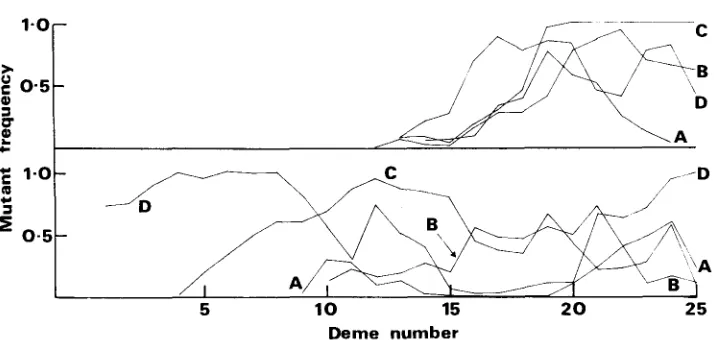
but those studies are of a model with recurrent mutations and the results are not directly interpretable in terms of allele frequencies.

The difference between the pattern of fixation for neutral and selected alleles is not necessarily apparent from a single set of allele frequencies. Gene flow in- duces a correlation in allele frequencies between demes, so that if there is a re- gion in which a neutral mutant reaches a high frequency, a cline will almost certainly be established. This is illustrated in Figure 2a, where an obvious cline is established and persists for several thousand generations. What distinguishes the neutral from the selected case is the temporary nature of such clines. Thus, the existence of a cline in allele frequencies without other evidence related to the genotypic fitnesses is not sufficient to imply selection. The persistence o r movement of such a cline would be, but that fact is of little use when only a single time sample is available.

(11)

SPATIAL DISTRIBUTION O F TRANSIENT ALLELES 803

Deme number

FIGURE 2.-Frequency of mutant us. deme number for two replicates of a neutral allele.

N = 50, n = 25, m = 0.02, and the mutant was introduced in deme 13. (A), 1000 gen.; (B), 2000 gen.; (C), 3000 gen.; (D), 6000 gen.

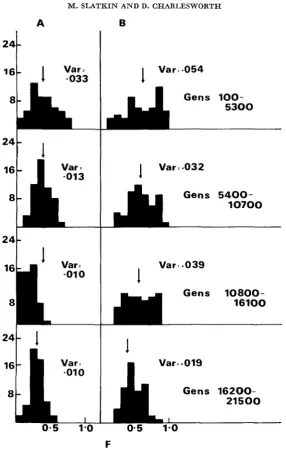
where j j and up2 are the mean and variance of the allele frequency at a given time.

The histograms were constructed by computing F at every one hundredth generation. We computed F both f o r all demes and for only those that were segregating. There is no obvious difference in the distribution of F at the beginning, middle and end of each run. Also, there is no difference from a case in which the allele is ultimately lost. These results for a stepping-stone model are similar to those of NEI, CHAKRAVARTI and TATENO (1977) for an island model.

(3) In the previous sections, we considered only a single, very simple pattern

of gene flow. There are two types of modifications to that pattern that can be made. We can allow short distance dispersal over more than one step, or we can allow changes in the geometric arrangement of the demes. Only the second possibility will be discussed in any detail. We found that, if migration of more than one step were permitted but there was a geometric decrease in the migration rates with the number of steps, then for comparable migration rates, there was no discernable difference in the pattern of loss and fixation from the one-step model. The effect of long distance migration will be discussed below.

We will consider the effect of changes in the geometric arrangement of demes only on selected alleles. There is already strong evidence from the simulations of

(12)

804 M. SLATKIN A N D D. CHARLESWORTH

A

24t

1

Var =

' l h 0 1 3

2 4 t

1

Var =

18 6 L

0 - 5 1.0

B

I

1

V a r : . 0 3 2

Var .039

1

Gens 1 0 8 0 0 -

1 6 1 0 0

1

Var. . 0 1 9

Gens 1 6 2 0 0 -

2 1 5 0 0

0-5 1 . 0

F

FIGURE 3.-Distribution of F values during four time intervals shown for a neutral mutant

going t o fixation. In (A), only segregating demes were used in computing F and in (B), all demes were used. Parameter values are the same as in Figure 2.

for selected alleles. For these reasons, we chose not to make the time-consuming runs of neutral mutants under diff errent dispersal patterns.

(13)

%

>

2

> r

E 2

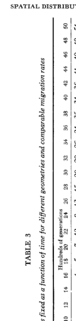
TABLE 3 Number of demes in which mutant is fixed as a funciion of time for diflerent geometries and comparable migration rates Hundreds of generations ReplicateNo. 2 4 6 8 10 12 14 16 18 PO 22 24 26 28 30 32 34 36 38 40 42 44 46 48 50

z

~~~ One-dimensional 1 1 5 7 12 8 13 15 20 20 26 24 35 34 36 41 40 49 51

2

model (51 demes, 2 3 3 3 19 13 19 18 25 23 33 30 35 39 37 46 48 47 51

2

0

m = 0.02) 3 5 4 10 10 15 17 17 19 26 31 32 33 36 51 Two-dimensional 1 1 19 39 92 93 IMI

r +I

model (100 demes 2 6 8 18 23 56 63 63 54 78 98 101)

0

5

m = 0.01) 3 2 22 48 72 80 75 100 (51 demes, 2 1 11 4.9 51 Island model 1 8 24 30 51 M m = 0.09.) 3 16 31 35 51

3

$

s

=

-

0.01.

(14)

806 M. SLATKIN A N D D. CHARLESWORTH

that the fraction of nonmigrants was the same. Thus, for m = 0.02 in one dimension, m = 0.01. in two and m 1=: 0.04 for the island model. The resulting values

for Pi are similar in character to those shown in Table 1, but there are some important differences. There were 1000 replicates for each of the three cases, and for the linear array, i = 2.94, while for the square array and the island model, i = 4.51 and 5.08, respectively. In addition, the mutant entered a maximum of 32 demes in the square array and 42 in the island model, as compared to only 14 for the linear array.

The effect of geometry on the Pi and i is best explained by the reduction in the probability that the mutant, if it is carried by a migrant, is carried to a deme where it is already present. This is clear from the simulation results because the higher values of 5 for the square array and island model are due to a very few of the replicates in which the mutant entered several demes. In such a case for the linear array, the mutant could be carried to only two additional demes at any time, while for the square array, the mutant could be carried to all the peripheral demes and for the island model, to all the remaining demes.

This effect of geometry is also clear from the process of fixation of advantageous mutants. In Table 3, the time course of fixation for three replicates for the same three cases is shown. As for the

Pi,

gene flow is much more effective in the square array and the island model. The difference between the latter two cases is much less than between either of them and the linear case. Thus, long distance dispersal would have a large effect on a one-dimensional array, but a much smaller one on a two-dimensional array of demes.

With the limited size of our simulations, we could not quantify the properties of the two-dimensional wave of advance. These is no analytic theory for the two-dimensional problem, and it would take a much larger array than we could manage to investigate properly the progress of a two-dimensional wave. How- ever, from our simulations it was obvious that, for the same selection coefficients and migration rates, the wave-like pattern was much less distinct and spatially structured in the initial stages in two dimensions than in one.

DISCUSSION

Although our simulation study is necessarily limited in scope, there are some patterns in the spatial distribution of transient alleles that seem to emerge and that might be of importance for interpreting data from natural populations. It is worthwhile to distinguish between rare alleles that are found in relatively few local populations and those that are common and found in all or almost all local populations. Assuming that all or almost all alleles are indeed transient, at least on a large enough time scale, then the first type will likely, but not certainly, be in the process of being lost and the second in the process of being fixed. To show this, we can plot Pi, the probability that, given that an allele is observed, it

(15)

SPATIAL DISTRIBUTION OF T R A N S I E N T ALLELES 807

With our simulation method, we could not consider the problem of recurrent mutations or the simultaneous presence of more than one type of mutant. How- ever, we are not considering any kind of frequency-dependent selection, so that it is a reasonable initial assumption that rare mutants in a population are independent of each other. For our results to be at all relevant for alleles that d t i - mately go to fixation, it must be the case that such mutants appear in a subdivided population at a particular locus sufficiently infrequently that each one can be considered independently. There is, of course: no evidence that this is so.

We can illustrate the kind of data to which our results can be applied. Unfor- tunately, there are not many studies in which suitable information is available. We show the

Pi

computed from the data of PRAKASH, LEWONTIN and

HUBBY

(1969) as summarized in LEWONTIN (1974, Table 26 and 27) for electrophoretic variants in Drosophila pseudoobscura in the western United States. There were twelve sites for which frequencies were estimated, but we did not use the results for two of them (Guatemala, GU and Bogata, BO) because they were too far from the remaining ten to be comparable. Our criterion f o r inclusion in Table 4

was that an allele has a frequency of less than 10% in at least two sites. In all,

0 - 5

0 4

r

c

Q .a

t

0 0-3

Y

0 - 2

0.1

s = - 0 1 ,Fixed

10 2 0 3 0 4 0 5 0

(16)

808

0 -

3 *

0 - 2

0

E

Q)

3

U

Q)

2 0 - 1

M. SLATKIN AND D. CHARLESWORTH

s=o

10 2 0

I

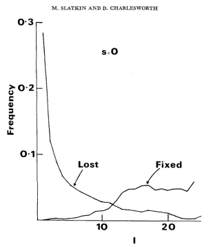
FIGURE 4.-Pi, the probability that, given that an allele is observed, it is observed in i demes, for alleles that are ultimately lost and those that are ultimately fixed. In all cases N = 50,

m = 0.02. For the neutral mutant, n = 25 and for the selected mutants, h = 0.5 and n = 51.

there were

43

such alleles, all of which would be included with any other reasonable criterion for rareness.

There are some obvious and important reservations in comparing Table

4

to our simulation results. It is well established, now, that electrophoretic variants are not necessarily single alleles (BERNSTEIN, THROCKMORTON and HUBBY 1973;

TABLE 4

Pimeasured for rare alleles in ten populations of Drosophila pseudmbscura

~

1 1 2 3 4 5 6 7 8 9 10

pi 0.233 0.093 0.186 0.046 0.046 0.046 0.186 0.0170 0.0701 0.023

(17)

SPATIAL DISTRIBUTION O F T R A N S I E N T ALLELES 809

SINGH, LEWONTIN and

FELTON

1976). In addition, so little is known about the

actual structure of most natural Drosophila populations that it is uncertain what sort of model of gene flow might be appropriate for comparison. Nevertheless, it is striking in Table 4 that Pi does not decrease at all rapidly with

i,

as is predicted from any of our models of population structure, in spite of the fact that the collection sites are widely separated. While we cannot use our results to propose an explanation for this pattern, it does seem to be an interesting and relevant problem that we hope stimulates further studies of actual spatial patterns of this type. Clearly, large scale movement of individuals, as has occurred

in humans, could lead to very different patterns of the

Pi.

For data on alleles that are common throughout the population range, the important question is whether or not there is a distinct clinal pattern. The presence of a cline in frequencies does not require selection, but it is difficult to explain the absence of clines in allele frequencies at polymorphic loci without assuming that selection coefficients are the same and possibly zero at every location and that sufficient time f o r the equilibrium state to be achieved. In the study of

D.

pseudoobscura cited above (LEWONTIN 1974, Tables 26 and 27), there is no apparent cline at any of the 13 polymorphic loci.

W e thank B. SCHULTZ for his typically cheerful and encouraging advice, and B. CHARLES- WORTH, M. NEI and the referees for helpful comments on an earlier draft of this paper. This research has been supported by Public Health Service Research Grant No. R01-GM22523, and

M. SLATKIN is supported by Research Career Development Award No. K01-GM00118.

LITERATURE CITED

BERNSTEIN, S. C., L. H. THROCKMORTON and J. L. HUBEY, 1973 Still more genetic variability

CHAKRABORTY, R. and M. NEI, 1974 Dynamics of gene differentiation between incompletely

CRUMP, K. S. and J. H. GILLESPIE, 1976 The dispersion of a neutral allele considered as a

EHRLICH, P. R. and P. H. RAVEN, 1969 Differentiation of populations. Science 165: 1228-1232.

FISHER, R. A., 1937 The wave of advance of an advantageous allele. Ann. Eugenics 7: 355-369.

FLEMING, W. H. and C. H. Su, 1974 Some one dimensional migration models in populations

HADELER, K. P., 1976 Travelling population fronts. pp. 585-592. In: Population Genetics and

HALDANE, J. B. S., 1948

KIMURA, M. and T. MARUYAMA, 1971

LATTER, B. D. H., 1973

LEWONTIN, R. C., 1974

LEWONTIN, R. C. and J. KRAKAUER, 1973

i n natural populations. Proc. Nat. Acad. Sci. U.S. 70: 3928-3931.

isolated populations of unequal sizes. Theoret. Pop. Biol. 5 : 440-469.

branching process. J. Appl. Prob. 13: 208-218.

genetics theory. Theoret. Popl. Biol. 5: 431-449.

Ecology. Edited by S. KARLIN and E. NEVO. Academic Press, New York.

The theory of a cline. J. Genet. 4.8: 277-284.

Pattern of neutral polymorphism in a geographically

The island model of population differentiation: a general solution.

The Genetic Basis of Evolutionary Change. Columbia U. Press, New

Distribution OI gene frequency as a test of the theory structured population. Genet. Res., Camb. 18: 125-131.

Genetics 73: 147-157.

York.

(18)

810

MARUYAMA, T., 1971a Analysis of population structure. 11. 2-dimensional stepping stone models

of finite length and other geographically structured populations. Ann. Hum. Genet. 35:

179-196. -, 1971b An invariant property of a geographically structured population. Genet. Res., Camb. 18: 81-84.

-

,

1974 A simple proof that certain quantities are independent of geographic structure of population. Theoret. Pop. Bio. 4: 148-154.

A note on the speed of gene frequency changes i n reverse directions in a finite population. Evolution 28: 161-163.

Mean and variance of F,, in a finite number of incompletely isolated populations. Thesret. Pop. Biol. 11 : 291-306.

Identity of genes by descent within and between populations under migration and mutation pressure. Theoret. Pop. Biol. 3: 460-465.

The molecular approach to the study of genic heterozygosity in natural populations. IV. Patterns of genetic variation in central, marginal and isolated populations of Drosophila pseudoobscura. Genetics 61 : 841-858.

Genetic heterozygosity within electrophoretic alleles of xanthine dehydrogenase in Drosophila pseudoobscura. Genetics 84.:

The rate of spread of an advantageous allele in a subdivided population. pp. 767-780. In: Population Genetics and Ecology, Edited by S. KARLIN and E. NEVO. Academic Press, New York.

The influence of gene flow and genetic distance. Am.

Naturalist 109: 597-601.

Corresponding editor: M. NEI iM.S L A T K I N A N D D. CHARLESWORTH

MARUYAMA, T. and M. KIMURA, 1974

NET, M., A. CHAKRAVARTI and Y. TATENO, 1977

NEI, M. and M. W. FELDMAN, 1972

PRAKASH, S., R. C. LEWONTIN and J. L. HUBBY, 1969

SINGH, R. S., R. C. LEWONTIN and A. A. FELTON, 1976

609-629. SLATKIN, M., 1976