On the Security of Protocols with
Logarithmic Communication Complexity
Michael Backes and Dominique Unruh Saarland University, Saarbrücken, Germany
{backes,unruh}@cs.uni-sb.de
Abstract. We investigate the security of protocols with logarithmic communication complexity. We show that for the security definitions with environment, i.e., Reactive Simulatability and Universal Composability, computational security of logarithmic protocols implies statistical security. The same holds for advantage-based security definitions as commonly used for individual primitives. While this matches the folklore that logarithmic protocols cannot be computationally secure unless they are already statistically secure, we show that under realistic complexity assumptions, this folklore does surprisingly not hold for the stand-alone model without auxiliary input, i.e., there are logarithmic pro-tocols that are statistically insecure but computationally secure in this model. The proof is conducted by showing how to transform an instance of an NP-complete problem into a protocol with two proper-ties: There exists an adversary such that the protocol is statistically insecure in the stand-alone model, and given such an adversary we can find a witness for the problem instance, hence yielding a com-putationally secure protocol assuming the hardness of finding a witness. The proof relies on a novel technique that establishes a link between cryptographic definitions and foundations of computational geometry, which we consider of independent interest.
Table of Contents
1 Introduction . . . 1
2 Notation and Security Models . . . 3
3 Indistinguishability of Logarithmic Random Variables . . . 5
4 Security with Environment . . . 5
5 Stand-Alone Security . . . 6
6 Advantage-Based Security . . . 12
A Correspondence Between Main Part and Appendix . . . 14
B Indistinguishability of Logarithmic Random Variables – Details and Proofs . . . 14
C Security with Environment – Details and Proofs . . . 17
D Stand-Alone Security – Details and Proofs . . . 27
D.1 On The Complexity of Finding a Good Adversary-Strategy . . . 28
D.2 Separation of Computational and Statistical Security Without Auxiliary Input . . . 41
D.3 The Stand-Alone Model With Auxiliary Input . . . 45
1 Introduction
In this work, we investigate the security of cryptographic protocols with logarithmic communi-cation complexity (logarithmic protocols for short). The central question we are aiming to solve is the following: Are there logarithmic protocols that are computationally secure but not statis-tically (information-theorestatis-tically) secure, i.e., can we base the security of logarithmic protocols on suitable complexity assumptions? At first glance, the answer seems obviously negative and constitutes a folklore in cryptography: If a protocol is not statistically secure anyway, and if all messages have logarithmic length, the protocol can be efficiently attacked by brute-force and hence cannot be computationally secure. We investigate whether this folklore indeed withstands a formal investigation. (Anticipating the answer: No, it does not in general.)
We consider the question in three different security models: security with environment, stand-alone security and advantage-based security. Security with environment is a family of very strin-gent security definitions, out of which the Reactive Simulatability framework and the Universal Composability framework constitute the most prominent members. Because of strong compo-sitionality results, security with environment has rapidly gained momentum in the last years. Stand-alone security on the other hand does not entail such strong compositionality guarantees, but it allows to derive suitable security guarantees for many cryptographic protocols for which security with environment is too strong a notion. Stand-alone security thus still constitutes one of the standard security notions in cryptography. Both security with environment and stand-alone security define security by comparing a protocol with some ideal specification. This intuitively guarantees that all properties enjoyed by the ideal specification are also fulfilled by the real protocol. In contrast, advantage-based security notions define a particular concrete property the protocol must satisfy. More precisely, one specifies a game and a well-defined goal, and then requires that every adversary only attains that goal with a sufficiently small probability (the so-called advantage). Stand-alone security is often seen as—and in fact was designed with the intuition of being—the union of all security properties fulfilled by the ideal specification. In other words, one expects a protocol to be stand-alone secure if for any advantage-based security notion that is fulfilled by the ideal specification, the real protocol also fulfils this property.
In the case of security with environment and of advantage-based security, we show that the folklore statement indeed holds true: For these notions, computational security implies statistical security. In the case of security with environment we prove this by showing that adversaries that randomly choose their communication are complete for logarithmic protocols, i.e., if there is some (possibly unbounded) adversary breaking the protocol, then the adversary using randomly selected messages also breaks the protocol. In the case of advantage-based security we analyse the protocol in a game-theoretic setting and show that an optimal strategy can efficiently be computed.
adversary is hard, too. In order to show that it is not only hard to find an adversary, but even that no efficient adversary exists, we additionally assume that efficiently computable sequences of hard instances of some NP-problem exist. We then construct a protocol that uses one of these instances for each security parameter. A successful efficient adversary would consequently be able to solve infinitely many of the hard instances, yielding a contradiction. Hence the resulting protocol is computationally secure but not statistically secure. This argumentation also holds for a uniform auxiliary input. However, in the case of nonuniform auxiliary input (in the sense of [Gol93]) the argument fails since we can encode the witness into the auxiliary input.
This separation has several interesting implications. First, it shows that the proof idea of breaking any logarithmic protocol with brute force does not work in general and that there are cryptographic problems that are more than exponentially hard in the length of the communica-tion. Second, since we showed that for advantage-based security notions computational implies statistical security, it follows that stand-alone security is more that just the union of all advantage-based security properties fulfilled by the ideal specification. This stands in contrast to the folklore point of view mentioned above, and it can even be seen as evidence that the intuition underlying the stand-alone model has not been fully met. Arguably the most interesting implication is the third one: Another folklore theorem states that ifP = NP(orBPP = MAto be more exact), cryptography becomes generally insecure in the sense that every statistically insecure protocol is also computationally insecure. However, the intuition underlying this statement is similar to the intuition of using a brute-force attack to break any logarithmic protocol. As we have shown the latter intuition to be unsound, it may be that a similar approach might also show the first one to be incorrect, i.e., it might be the case that even ifP = NPandBPP = MA, computationally secure protocols exist that are not statistically secure.
Related Work. The paper that comes closest to our work is [Unr06]. There it was shown that for
security with environment and polynomial-time protocols, statistical security and security with respect to exponential-time adversaries coincide. This is analogous to our result for the setting of security with environment, only one level higher in the complexity hierarchy. Note however that directly applying their technique to the setting of logarithmic protocols yields a weaker result than the one we achieve when dealing with security with environment: For protocols that have logarithmic communication complexity and run in logarithmic time, computational security with environment implies statistical security with environment. However, the results in [Unr06] still served as the inspiration for analysing the security of logarithmic protocols.
framework [PW01, BPW04] and the Universal Composability (UC) framework [Can01, Can05], which both pursue the idea of augmenting the stand-alone model with an environment that es-sentially ensures security in arbitrary surrounding contexts in which the protocol under consider-ation is executed. This security with enviroment can be shown to entail strong compositionality guarantees and has proven successful in analyzing various cryptographic primitives and pro-tocols. Advantage-based definitions of cryptographic primitives have been playing a key role from the very start in essentially all cryptographic definitions, e.g., semantic security [GM84], CMA-security of signatures [GMR88], and many more.
Outline. In Section 2, we present the notation and security definitions used in the subsequent
sections. In Section 3 we give an intermediate result: If random variables of logarithmic length are computationally indistinguishable, they are also statistically indistinguishable. In Section 4 we show that for logarithmic protocols, computational security with environment implies statis-tical security with environment. In Section 5 we show that for stand-alone security, this does not hold in general. We construct logarithmic protocols that are computationally stand-alone se-cure without auxiliary input but not statistically stand-alone sese-cure. In the presence of auxiliary input, we show that if a logarithmic protocol is computationally stand-alone secure, it is also statistically stand-alone secure. In Section 6 we show that for advantage-based security notions, computational security implies statistical security.
2 Notation and Security Models
Notation. The real numbers are denoted R, the natural numbers by N = {1,2, . . .}. The statistical distance between X and Y we denote∆(X;Y). Two families of random variables
{Xz}z∈Z and{Yz}z∈Z are statistically indistinguishable if∆(Xz;Yz)is negligible in|z|. The
families {Xz}z∈Z and {Yz}z∈Z are computationally indistinguishable if for any probabilistic
polynomial-time algorithmD the difference|Pr[D(z, Xz) = 1]−Pr[D(z, Yz) = 1]|is
negli-gible in|z|. A family{Xz}z∈Z is efficiently constructible if there is a probabilistic
polynomial-time algorithmSsuch thatS(z)has distributionXz. IfZ =N, we interpretz∈Nas its unary encoding1z.
IfAandBare interactive Turing machines (ITMs), we writehA, Bifor the output ofB in an execution ofAandB. We writehhA, Biifor the pair consisting of the outputs ofAandB. If
AandBtake some inputxandy, we writehA(x), B(y)iandhhA(x), B(y)ii. For two vectorsx, y∈R
n, we writehx, yi:=P
ixiyifor their inner product. Thel1-norm
ofxwe writekxk1 := Pi|xi|. Thel1-distance is writtend1(x, y) := kx−yk1. For a matrix
S := (sij)∈ R
m×n, lets
i·denote itsith row. Given two setsX, Y ⊆R
nand a scalarα ∈
R, we writeX+Y :={x+y :x ∈X, y ∈Y}andαX :={αx:x∈X}. A subsetX ⊆R
nis
a halfspace if it has the formX ={x :hc, xi ≤ b}, andXis called a polytope if it is bounded and the intersection of finitely many halfspaces.
Security models. An important class of security models are the security models with
an honest userH(also known as the environment). The sequence of all internal states ofHand messages sent and received byHis called its view and writtenviewπ,A,H,k(H). Herek∈Nis the security parameter available to all machines. For a detailed definition we refer to [BPW04]. In the Reactive Simulatability framework, security is then defined as follows:
Definition 1 (Reactive Simulatability (sketch)). A protocol π is as secure as a protocol
ρ with respect to computational universal reactive simulatability if for every polynomial-time machine A (the adversary) there is a polynomial-time machine S (the simulator) such that for every polynomial-time machine H (the honest user) viewπ,A,H,k(H)
k∈N and
viewρ,S,H,k(H)
k∈N
are computationally indistinguishable ink.
We speak of statistical universal reactive simulatability if in the above definitionsA,Hand
S are unbounded and statistical indistinguishability is used instead of computational indistin-guishability.
Other variants of security models with environment exist, e.g. general reactive simulatability where the simulator may depend on the honest user [BPW04], and UC security, which is similar to Definition 1 but formulated in the UC framework [Can05].
Another very common security definition is stand-alone security. It is weaker than the se-curity models with environment, and many useful protocols are only stand-alone secure. Since there are many variants of stand-alone security (e.g., [Can95, Gol04]), we work with the follow-ing generalised definition.
Definition 2 (Stand-Alone Security). Let π and ρ be ITMs. We say that π is as secure as ρ with respect to computational stand-alone security with auxiliary input, if for every polynomial-time ITM A (the adversary) there is a polynomial-time ITM S (the simulator) such that for sequences x and z of strings of polynomial length, the families of distributions
hhA(1k, zk), π(1k, xk)ii k,zk,xk and
hhS(1k, zk), ρ(1k, xk)ii k,zk,xk are computationally
in-distinguishable ink.
We speak of statistical stand-alone security with auxiliary input if the above holds with un-boundedAandS and statistical indistinguishability.
We speak of computational/statistical stand-alone security without auxiliary input if A
and S do not get the additional input zk (i.e. the distributions hhA(1k), π(1k, xk)ii and hhS(1k), ρ(1k, xk)iiare compared).
Depending on the variant of stand-alone security we consider, the protocolsπandρdo not only incorporate the actual behaviour of all uncorrupted parties, but also mechanisms for delivering messages, corrupting parties and—of specific importance for the ideal model—passing inputs to the corrupted parties. In many definitions, the ideal protocolρis not allowed to be an arbitrary protocol, but only a probabilistic function. This can be realised by requiring ρ to receive only one message (corresponding to the input from the simulator) and to send only one message (to pass the output of the corrupted parties to the simulator). Our construction in Section 5 is of that form.
Definition 3 (Advantage-Based Security). LetBbe an ITM andγa function. We say thatBis
γ-secure with respect to computational advantage-based security with auxiliary input if for every polynomial-time ITMAand for all sequencesxandzof strings of polynomial length, there is a negligible functionµsuch thatPr[hA(1k, zk), B(1k, xk)i= 1]≤γ(k) +µ(k)for allk∈N.
We speak of statistical advantage-based security if the above holds with unboundedA. We speak of advantage-based security without auxiliary input ifAdoes not get the additional inputzk(i.e., the distributionhA(1k), B(1k, xk)iis considered).
In this definition, the ITMBtakes the role of both the protocol under consideration and the game defining the desired security property. In the definition of, e.g., IND-CPA security, B would expect two plaintexts from A, encrypt one of them, and then output if the adversary guesses correctly which plaintext was encrypted.
3 Indistinguishability of Logarithmic Random Variables
Before analysing more complex security notions, we start by investigating the indistinguisha-bility of random variables. For random variables of logarithmic length, statistical and compu-tational indistinguishability coincide. This fact will be useful in the equivalence proofs for the more complex security notions.
Theorem 4 (Indistinguishability of Logarithmic Random Variables). LetZ ⊆ {0,1}∗. Let
X = {Xz}z∈Z andY = {Yz}z∈Z be efficiently constructible families of random variables of
logarithmic length.
IfX andY are computationally indistinguishable, then they are statistically indistinguish-able.
Proof (sketch). IfX and Y are statistically distinguishable, there is a polynomial p such that
∆(Xz, Yz) ≥ 1p for infinitely many lengths |z|. SinceXz andYz have a range of polynomial
size we can approximate the distribution ofXz and Yz using a polynomial number of samples
with an expected error of 1q where q is an arbitrary polynomial. Given an explicit description of the true distributions ofXz andYz, we can efficiently derive an optimal distinguisher: Upon
input x, determine whetherxis more likely when drawing from Xz or from Yz. If we use the
approximated distributions instead, the resulting efficient distinguisher D is not optimal any-more, but for sufficiently largeq, the error introduced by the approximation is at most 21p, so
|Pr[D(Xz) = 1]−Pr[D(Yz) = 1]| ≥∆(Xz, Yz)−21p ≥ 21p infinitely often. ThusXandY are
computationally distinguishable. ut
4 Security with Environment
general. However, in the case of logarithmic communication complexity, the set of all possible communication traces has polynomial size, so the probability of randomly guessing a given communication trace is noticeable. Then, if a (possibly unbounded) environmentEsucceeds in distinguishing the real and the ideal protocol, an environmentE˜that simply guesses all messages thatEsends can be shown to be a successful distinguisher, too. This is captured in the following lemma.1
Lemma 5. LetXandY be oracle Turing machines. LetAbe an oracle. Assume bothXandY
call their oracle at mostrtimes, and that the total length of the answers given byAis at most
l. Assume further that all oracle queries and oracle answers can be extracted from the output of
XandY. LetA˜be the oracle that first uniformly choose anr-tupel(o1, . . . , or)of strings such
that the total lengthP
oi is at mostl, and then upon itsi-th activation responds withoi. Then ∆(XA˜;YA˜)≥2−O(l+r)∆(XA;YA).
This lemma is proven by induction over the number of rounds.
The construction in this lemma represents the essentials of the definitions of Reactive Simu-latability and UC (and probably other flavours of security with environment). The oracleA(or
˜
A) represents the environment, whileX and Y represent the real and the ideal protocol execu-tion. More exactly, the machineXcontains the complete real model, including adversary, real protocol and the underlying network model, while all messages sent to the environment are re-alised as oracle calls toA. Similarly, the machineY contains the simulator, the ideal protocol and the underlying network model. In this light, Lemma 5 states that (independent of adversary and simulator), we can replace any environment by an environment that randomly chooses its messages, and which hence runs in probabilistic polynomial time. Additionally exploiting that the view of the environment has logarithmic length, and hence that computational and statisti-cal indistinguishability of the views of the environment coincide by Theorem 4, we obtain the following theorem:
Theorem 6 (Computational Implies Statistical Simulatability/UC). Let π and ρ be polynomial-time protocols with logarithmic communication complexity. Assume thatπis as se-cure asρwith respect to computational universal Reactive Simulatability. Thenπis as secure as
ρwith respect to statistical universal reactive simulatability. The same holds for general reactive simulatability and for UC.
5 Stand-Alone Security
Surprisingly, the results of the preceding section do not apply to the stand-alone model (without auxiliary input): Under realistic complexity assumptions, there are logarithmic protocols that are statistically insecure, but computationally secure. (In this section, security always means stand-alone security without auxiliary input.) The random adversary we used in the previous section does not work in this case as illustrated by the following example: Consider the insecure coin-toss protocol where Bob randomly chooses the outcome and sends it to Alice. An adversary
1
However, in the actual proof the factor by which the statistical distance is reduced is not the probability of guessing a given communication, but instead3−r
that randomly chooses its messages would—in the case of a corrupted Bob—choose a random outcome, which corresponds to Bob’s honest behaviour.
To prove the separation, we give a construction that transforms a yes-instance of the set cover problem into a protocol with two properties: There exists an adversary such that the protocol is statistically insecure, and given such an adversary we can find a witness for the set cover instance. Consequently, such a protocol is computationally secure unless such witnesses can be found in probabilistic polynomial time.
Definition 7 (Set Cover). Letn ∈ N,sij ∈ {0,1}with i = 1, . . . , mand j = 1, . . . , nand
d ≤ n. Let si· 6= 0 for alli = 1, . . . , m. Then (n, m, S, d) is an instance of set cover (with
S:= ((sij))). LetSj :={i:sij = 1}. Then(n, m, S, d)is a yes-instance of set cover if there is
a setC ⊆ {1, . . . , n}such that#C≤dandS
j∈CSj ={1, . . . , m}.
Set cover is well-known to be NP-complete. To describe our construction in more detail, we first define the class of good adversaries, namely those that perform an attack that cannot be simulated.
Definition 8 (Good Adversaries). LetπandρandAbe ITMs, and letε >0. We callA ε-good for(π, ρ)if for all ITMsSthe statistical distance betweenhhA, πiiandhhS, ρiiis bounded from above byε. We callAgood for(π, ρ)ifAisε-good for someε >0. Strongly good adversaries are defined analogously, withhA, πiandhS, ρiinstead ofhhA, πiiandhhS, ρii.
Obviously, a protocolπ is statistically as secure as a protocolρif and only if there is a negligi-ble function εsuch that A(1k) isε(k)-good for(π(1k), ρ(1k)). The stricter notion of strongly
good adversaries represents adversaries for which already the protocol output (without the ad-versary’s/simulator’s output) is distinguishable in the real and the ideal model. So intuitively, a strongly good adversary breaks the correctness and not only the secrecy of the protocol. However, the protocols we are going to construct will not keep any secrets from the adversary/simulator, so good and strongly good adversaries coincide in this case. Our goal at this point is to transform a given set cover instance into a protocol pair such that good adversaries correspond to witnesses. (At this point, we are interested in protocols that are not parametrised by the security parameter. Later, a sequence of set cover instances will be used to construct a parametrised protocol.)
For our transformation, we interpret the property of being a good adversary geometrically. With any protocol πwe associate the set of all probability distributions ofπ’s output when run with different adversaries. We consider these distributions as points in an Euclidean space as follows: for an ITM T whose output lies in the set{1, . . . , t}, we consider p := hA, Ti as a vector inR
tby settingp
i:= Pr[hA, Ti=i]. This gives rise to the following definition:
Definition 9 (Adversary-Polytope). The adversary-polytopeAT ⊆R
tof the ITMT is defined
asAT :={hA, Ti:Ais an ITM}.
We can now reformulate strongly good adversaries geometrically: An adversary A is strongly good for(π, ρ)ifhA, πi ∈/ Aρ, and it is stronglyε-good ifd1(hA, πi,Aρ)≥2ε. So the problem
adversaryA is stronglyε-good if and only ifkhA, πik1 ≥ l+ε. So in this case, the question whether strongly ε-good adversaries exist can be reduced to the problem of estimating the size ofAπ (w.r.t. thel1-norm).2However, estimating the size of a polytope is hard in general: Let a
set cover instance(n, m, S, d)be given. LetP∗ ⊆R
nbe the polytope defined by the following
inequalities: x ∈ P∗ if 0 ≤ xj ≤ 1, Pxj ≤ d, and for all i = 1, . . . , m: Pxjsij ≥ 1. If
we associate a point v ∈ {0,1}n with a set C := {i : vi = 1}, it is easy to see that such a point v is in P∗ if and only if C is a witness for the set-cover instance. Since v ∈ [0,1]n
is in {0,1}n if and only if d
1(v, u) = n2 whereu := (12, . . . ,21)T, and d1(v, u) ≤ n2 for all
v ∈[0,1]n, if follows thatkP∗−uk1 ≥ n2 if and only if(n, m, S, d)is a yes-instance, and any pointv∈P∗withd1(v, u)≥ n2 gives us a witness for that set cover instance. Moreover, it turns out that approximatingkP∗−uk1up to an additive constant is already sufficient. Unfortunately we cannot construct protocols that haveP∗ as their adversary-polytope (for some no-instances
(n, m, S, d),P∗ is empty, which cannot happen for adversary-polytopes). Fortunately, requiring the equations definingP∗to hold only approximately still allows to reduce the set cover instance to it, and the resulting polytope can be constructed as an adversary-polytope as we will see below.
Definition 10 (Set Cover Polytope). Letε ∈ (0,1). LetP be a polytope. We call P an ε-set cover polytope for(n, m, S, d)if the following holds:
– P ⊆[0,1]n.
– Letv∈ {0,1}n. Ifkvk
1 ≤dandhsi·, vi ≥1for alli= 1, . . . , m, thenv∈P.
– Letv∈[0,1]n. Ifkvk1 > d+ 1−εorhsi·, vi < εfor somei∈ {1, . . . , m}, thenv /∈P.
Obviously,P as constructed above is anε-set cover polytope for anyε∈(0,1).
Lemma 11 (Reducing Set Cover to Polytope 1-Norm). LetP be anε-set cover polytope and letP0 :=P−12u. Then there is aδ ∈Ω(ε/poly(n))such that
(i) If(n, m, S, d)is a yes-instance, thenkP0k1= n
2. (ii) If(n, m, S, d)is a no-instance, thenkP0k1 ≤ n2 −δ. (iii) Moreover, given a vectorv∈R
nwithd
1(v, P0)< δandkvk1> n2 −δ, we can efficiently compute a witness for(n, m, S, d).
Assume the real protocol has adversary-polytopeP0as in Lemma 11, and the adversary-polytope of the ideal protocol is the cross-polytope X ={x :kxk1 ≤ n2 −δ2}. Then if(n, m, S, d)is a yes-instance, by Lemma 11 there is av∈P0withkvk1 = n
2. SinceP0is the adversary-polytope of the real protocol, there exists a stronglyδ-good adversary as seen above. Conversely, ifAis a good adversary, we havehA, πi ∈ P0 and khA, πik1 ≥ n
2 −2δ. With black-box access toA, we can efficiently sample the distribution hA, πiwith error δ2 (w.r.t. thel1-norm). This gives a pointv satisfying the conditions of Lemma 11 (iii) and hence yields a witness for(n, m, S, d). The results we achieved so far are summarised as follows:
Lemma 12 (informal). Assume that we can construct protocolsπandρsuch that the adversary-polytope ofπis anε-set cover polytope, and the adversary-polytope ofρis a cross-polytope (of
2
Of course, since0 ∈ X and0does not correspond to a valid probability distribution, the setX cannot be an adversary-polytope. This problem can be solved by down-scalingAandS and embedding them into the subset ofR
n+1corresponding to the set of probability distributions. We will ignore this issue in this proof outline and pretend that all pointsv∈R
n
(a) (b) (c) (d)
+ + =
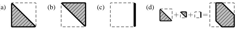
Fig. 1. Polytopes for set cover instance (n, m, S, d) with n = m = 2,d = 1, S1 = {1,2},
S2 ={1}. (a) PolytopeDenforcing the condition that the set cover consists of at most one set (d= 1). (b) PolytopeS1enforcing that the set cover contains setS1orS2(because1is contained in both). (c) PolytopeS2enforcing that the set cover containsS1(because2is only contained in
S1). (d) PolytopePε= (1−2ε)D+εS1+εS2enforces all aforementioned conditions. The only
remaining square-vertex is(1,0), corresponding to the only witnessC={1}of(n, m, S, d).
suitable size). Then there is a strongly δ-good adversary if(n, m, S, d) is a yes-instance, and given a strongly good adversary we can efficiently compute a witness for(n, m, S, d).
Constructing the cross-polytope is easy: The cross-polytopeXinR
nhas2nverticesv
1, . . . , v2n.
We construct the protocolρas follows: Upon first activation,ρexpects ani∈ {1, . . . ,2n}from the adversary and then chooses its output according to the distributionvi. By choosing a suitable
distribution fori, the adversary can achieve any convex combination of thevi, so the
adversary-polytope is their convex combination X. Sincei can be transmitted using O(logn) bits, the communication complexity ofρis logarithmic.
Constructingπis more difficult. In general, we cannot expect a set cover polytope to have a polynomial number of vertices, so the approach used forρfails. Instead, we have to investigate in more detail which adversary-polytopes can be constructed. First, every polytope consisting of a single point{v}can be constructed: the corresponding protocol chooses its output according to the probability distribution v (we call this the singleton-construction). Second, if we can construct the polytopes P1, . . . , Pr, we can also construct the convex hull P of their union: The corresponding protocol expects an i ∈ {1, . . . , r} from the adversary and then executes the protocol having adversary-polytope Pi (union-construction). This is a generalisation of the
construction ofX above. Third, we can also constructα1P1 +· · ·+αrPr where Pαi = 1,
αi ≥0: The protocol randomly chooses aniwith probabilityαi(sum-construction). In all cases
we assume that whenever the protocol makes a random choice, it informs the adversary about the outcome of that choice.
To construct a set cover polytope, we first assume that we are able to construct poly-topes for each defining inequality independently. That is, we assume that we can construct the upper bound polytope D := {v ∈ [0,1]n : kvk
1 ≤ d} and the lower bound polytope
Si :={v∈[0,1]n:hs
i·, vi ≥1}. The intersection of these polytopes isP∗which we saw above to be a set cover polytope. Unfortunately, we cannot make use of this fact, since we cannot efficiently construct the intersection as an adversary-polytope. We instead define the combined polytopePε := (1−mε)D+Pmi=1εSiwhich can be constructed fromDandSiusing the
sum-construction. Since there are onlym+1summands, the communication complexity isO(logm). It is left to see thatPεis anε-set cover polytope.
The actual proof is by verifying all inequalities required by Definition 10. For the proof sketch, we instead try to give some geometric motivation (see Figure 1 for an example). First, since the polytopes Dand Si are enclosed in the unit cube[0,1]n, so isP
ε(since the factors in the
construction ofPεadd up to1). Furthermore, letv∈ {0,1}nbe a cube-vertex that should not be
included inPε(either becausekvk1 > dor becausehsi·, vi<1). Then in at least one summand
RofPε(i.e.,Dor one of theSi), the cube-vertexvis “cut off” by the inequality definingR. It follows that in the sumPεthat corresponding vertex is also cut off. Finally, if we chooseεsmall
enough, not too much is cut off, so all cube-vertices that must be contained inPεaccording to
Definition 10 are preserved. For a full geometric understanding of the construction, we suggest to examine the example in Figure 1 or the interactive3D-example in [BU06].
It is left to show that we can construct D and Si as adversary-polytopes. We will only
sketch the construction of D; the polytope Si is constructed similarly. The vertices ofD are
V := {v ∈ {0,1}n : kvk
1 ≤ d}. Again, D has an exponential number of vertices, so a direct construction as done forXis not possible. However, each vertexvcan be considered as a word of lengthnand Hamming-weight at most d. If we decompose vinto its left and right halves vl and vr, we get two words of length n2 and weights dl, d2 with dl +dr ≤ d. Thus
V =S
iVi×Vd−iwhereiranges (at most) over{0, . . . , d}andViis the set of words of length n
2 and weight at mosti. Since eachViis again a set of the same structure asV, we can recursively apply that decomposition and constructV from sets of words of length1. Furthermore, if we again consider V as a subset of R
n, it is V = S
iVi+Vd−i if we embed the n2-dimensional setsVi andVd−i suitably intoR
n. More exactly, the left summand V
i is embedded intoR
nas Vi×R
n/2and the right summandV
d−iis embedded asR
n/2×V
d−i. The recursion is preserved
when we take the convex hull, i.e., convV = S
iconvVi + convVd−i. Since D = convV
we found a recursive construction of D from one-dimensional sets that uses only the unions and sums. The one-dimensional sets have a constant number of vertices and can therefore be directly constructed. The unions can be handled using the union-construction. The sums however cannot be implemented directly. The sum-construction does not allow to construct convVi + convVd−i, but only 12convVi+ convVd−i. As a consequence, the resulting polytope is notD,
but D scaled by the factor 2−O(logd) where O(logd) is the depth of the recursion. However, this problem is easily solved by accordingly scaling all other constructions. The communication complexity for realising D is O(logn) rounds, and O(logn) communication in each round (the adversary has to choose the index iin the union-construction). This gives communication complexityO((logn)2)which is not logarithmic. Summarising, we can construct a protocolπ withO((logn)2) communication complexity that has adversary-polytopePε. With Lemma 12
we get:
Lemma 14 (informal). There are protocolsπandρwith communication complexityO((logn)2)
such that the following holds: There is a stronglyΩ(1/poly(n))-good adversary if(n, m, S, d)
is a yes-instance, and given a strongly good adversary we can efficiently compute a witness for
(n, m, S, d).
nO(logn)-time, it follows that solving set cover instances withn:= 2√logkis hard inO(poly(k)) -time. By construction, the protocolsπandρshare all information with the adversary. From this it can be derived that an adversary is good for(π, ρ)if and only if it is strongly good. Combining these observations with Lemma 14 and the NP-completeness of set cover, we get the following theorem:
Theorem 15. If NP 6⊆ BPTIME(nO(logn)), the following holds for all ε > 0: There is no efficient probabilistic algorithm that finds a good adversary for a pair of polynomial-time algo-rithms with logarithmic communication complexity, even when they are guaranteed to have a stronglykε-good adversary.
This result already almost separates statistical and computational security for logarithmic pro-tocols. However, two problems still have to be solved. First, a separation not only requires that it is hard to find a good polynomial-time adversary, but that such an adversary does not even exist. Second, an adversary may not be good while still being successful in distinguishing the real and the ideal protocol, because the simulator (which is also computationally bounded) does not simulate optimally. The second problem can be solved by showing that at least for the proto-cols constructed here, there exists an efficient black-box simulator that simulates perfectly if the adversary is not strongly good. To solve the first problem, however, we have to strengthen our assumption:
Assumption 16. There exists a sequencefn of Boolean formulas computable in deterministic
polynomial time such that infinitely manyfnare satisfiable and such that for any probabilistic
Turing machineAthat runs innO(logn)-time, the probabilityPr[f
n(A(1n)) = 1]is negligible in n.
We now construct protocolsπ˜ and ρ˜which on input the security parameterkcomputef2√log k,
convert it into a set cover instance and then runπorρ, respectively, on this instance. As infinitely manyfnare satisfiable, stronglyΩ(1/poly(2
√
logk))-good adversaries exist infinitely often by
Lemma 14. Soπ˜is not statistically as secure asρ˜. However, if some polynomial-time adversary was good for infinitely many k, we could use Lemma 14 to find witnesses for fn with
non-negligible probability inn. This yields the following theorem:
Theorem 17 (Computational Does Not Imply Statistical Stand-Alone Security Without Auxiliary Input). If Assumption 16 holds, computational stand-alone security without auxiliary
input does not imply statistical stand-alone security without auxiliary input for polynomial-time protocols with logarithmic communication complexity.
It is easy to see that this result also holds in the case with uniform auxiliary input (in the sense of [Gol93]). However, Theorem 17 does not cover the case with nonuniform auxiliary input. This reason is that Assumption 16 cannot hold for nonuniform adversaries. In fact, if we allow a nonuniform input it turns out that whenever a good (but potentially unbounded) adversary exists, its strategy can be encoded into the auxiliary input. For details, see Appendix D.3. This yields the following result:
and the length of the output ofπandρon input(1k, z)is logarithmic ink. Ifπ is as secure asρ
with respect to computational stand-alone security with auxiliary input, thenπis as secure asρ
with respect to statistical stand-alone security with auxiliary input.
6 Advantage-Based Security
In the case of advantage-based security, we show that statistical and computational security coin-cide. The basic idea of our proof is as follows. A protocolBas in Definition 3 can be considered as a one-player-gameGB, the adversaryAbeing the player. The payoff of the game is the output
ofB. Then the expected payoff for a given adversaryAis the advantagePr[hA, Bi= 1]. Thus an optimal strategy for the gameGBcorresponds to an adversary with maximal advantage. If we
can show that a nearly optimal strategy forGBcan be found in polynomial time, it follows that for any successful adversary, there is a successful polynomial-time adversary, and thus statistical and computational security coincide.
Two obstacles have to be overcome. First, in the advantage-based security definition,Bhas an input, while in the game-theoretic setting, the concept of an external input to the game does not exist. However, when inspecting the definition of advantage-based security, we see that the inputxis chosen jointly with the adversary, so we can assume it to be chosen by the adversary. Since we assume a logarithmic bound onB’s communication complexity, there is a polynomial
nsuch that the length ofxis bounded by logn. Moreover, we deal with a sequence of games, parametrised by the security parameter, giving rise to the following definition:
Definition 19 (Game of a Protocol). LetBbe an ITM. The gameGBk,nof the protocolBis the following one-player game:
– First, player 1 may choose a stringxwith|x| ≤logn.
– Then, the game consists of the interactionhA, B(1k, x)i, where player 1 learns all messages thatAreceives, and may choose all message thatAsends.
– The payoff of the game is1ifBoutputs1, and0otherwise.
This of course does not yield a one-to-one correspondence between optimal adversaries and (sequences of) optimal strategies anymore. A strategyµincorporates an inputx, while the cor-responding adversaryAGonly implements the behaviour after choosingx. Nevertheless, for an adversaryAGcorresponding to an optimal strategy, we get
max
|x|≤lognPr[hA
G(1k), B(1k, x)i]≥ max
A,|x|≤lognPr[hA(1
k), B(1k, x)i]
since the maximum ranges over allx, in particular over the one thatµwould have chosen. (Here we use that µ can be assumed to be deterministic.) Since B has logarithmic communication complexity, the game tree ofGBk,nhas polynomial size. For one-player-games optimal strategies can be found in polynomial-time in the size of the game tree, yielding the following result (both in the case with and without auxiliary input):
The second obstacle is the fact that in general we cannot efficiently compute the game tree ofGB
k,n. We remedy this problem by sampling the probabilities in the game tree yielding an
approximation. Ifµis an optimal strategy for the approximated game, then the expected payoff ofµ in the original game is at most 1p below the optimum wherep is a polynomial we may choose. IfB is statisticallyγ-insecure, there is an adversary Asuch that (omitting arguments)
Pr[hA, Bi]≥γ+1q infinitely often for some polynomialq. By chosing e.g.,p:= 2q, it follows thatPr[hAG, Bi]≥ γ+ 21q. SinceAG runs in polynomial time, computationalγ-insecurity of
Bfollows. Concluding, we have the following result:
Theorem 21 (Computational Implies Statistical Advantage-Based Security). Let B be a polynomial-time ITM that upon input (1k, x) has logarithmic communication complexity in k
and reads only a prefix ofxof logarithmic length ink. Assume thatBisγ-secure for some func-tionγ with respect to computational advantage-based security without auxiliary input. ThenB
A Correspondence Between Main Part and Appendix
To make the appendix more readable, we have repeated most of the definitions and theorems from the main part of this paper in the appendix (sometimes in greater detail). To make it easier to find details and proofs for a definitions or theorem in the main part of the paper, we give the correspondences between the main part and the appendix in the following table.
Main part Appendix
Definition 1 Definition 24 on page 17 Definition 2 Definition 31 on page 27 Definition 3 Definition 61 on page 47 Theorem 4 Theorem 23 on page 15
Lemma 5 Lemma 27 on page 24
Theorem 6 Theorems 29 and 30 on pages 24 and 26, resp. Definition 7 Definition 35 on page 28
Definition 8 Definition 34 on page 28 Definition 9 Definition 33 on page 28 Definition 10 Definition 36 on page 29 Lemma 11 Lemma 37 on page 29
Lemma 12 No exact correspondence. Implicit in the proof of Theorem 49 on 38
Lemma 13 Lemma 39 on page 30 Lemma 14 Theorem 49 on page 38 Theorem 15 Corollary 51 on page 40 Assumption 16 Assumption 52 on page 41 Theorem 17 Theorem 58 on page 44 Theorem 18 Theorem 60 on page 46 Definition 19 Definition 62 on page 47
Lemma 20 No exact correspondence. Implicitly contained in the proof of Theorem 69 on page 52
Theorem 21 Theorem 69 on page 52
B Indistinguishability of Logarithmic Random Variables – Details and Proofs
Before we can prove that for efficiently sampleable random variables of logarithmic length com-putational and statistical indistinguishability coincide, we first need the following lemma that states that the distributions of such random variables can be estimated sufficiently well.
Lemma 22 (Estimation of Random Variables). LetZ ⊆ {0,1}∗. LetX = {Xz}z
∈Z be an
efficiently constructible family of random variables of logarithmic length in|z|.
Then there exists a probabilistic polynomial-time algorithmSX with the following property:
Upon input(z,1f), the algorithmS
X outputs the description of a probability distributionX˜,
Proof. Letl(k)≥1be an efficiently computable logarithmic bound on the length ofXzfor all |z|=k. LetMkbe the set of all strings of length at mostl(k). (Then we always haveXz ∈M|z|.) Note that#Mkis polynomially bounded ink.
We defined the algorithmSX as follows: On input(z,1f), letn:= 161 ·#M|3z|·f3and choose independent valuesx1, . . . , xn distributed according toXz. LetPx := #{i≤ n :xi =x}/n
be the relative frequency ofx in our sample. Output the probabilities {Px}x∈M|z| as rational
numbers. (I.e., thePx define a distributionX˜ withPr[ ˜X =x] =Px.)
Obviously, we haveP
xPx = 1, thusX˜ is a probability distribution.
Fix somez∈Zandf ∈N. Sincen·Pxhas(n, p)-binomial distribution forp:= Pr[Xz =
x], we haveE[nPx] =npandVar[nPx] =np(1−p)≤ n4. HenceE[Px] =pandVar[Px]≤ 41n.
From this it follows that for anyz∈Z, it holds that
Pr
∃x∈M|z|:|Px−Pr[Xz =x]|> f·#2M |z|
≤ X
x∈M|z| Pr
|Px−Pr[Xz =x]|> f·#2M |z|
≤ X
x∈M|z| Pr
Px−E[Px] ≥
4√n f·#M|z| ·
p
Var[Px]
(∗)
≤ X
x∈M|z|
f2·#M2 |z|
16n =
f2·#M3 |z|
16n =
1 f.
Here(∗)is an application of Chebyshev’s inequality.
Therefore the following holds with probability at least1−1f:
∀x∈M|z|:|Px−Pr[Xz =x]| ≤
2 f·#M|z|
. (1)
If (1) holds, we have
∆( ˜X;Xz) = 12
X
x∈M|z|
|Px−Pr[Xz =x]| ≤ 12·#M|z|·
2 f·#M|z| =
1 f.
Since (1) holds with probability at least1−f1, the lemma follows. ut We can now prove that for efficiently sampleable random variables of logarithmic length computational and statistical indistinguishability coincide.
Theorem 23 (Indistinguishability of Logarithmic Random Variables). LetZ ⊆ {0,1}∗. Let
X = {Xz}z∈Z andY = {Yz}z∈Z be efficiently constructible families of random variables of
logarithmic length.
Proof. Assume thatXandY are computationally indistinguishable.
LetSX and SY be algorithms as in Lemma 22. We define a probabilistic polynomial-time
algorithm D as follows: On input(z,1f, x), invoke d
X ← SX(z,1f) and dY ← SY(z,1f).
ThendXanddY are the descriptions of some distributionsX˜andY˜. IfPr[ ˜X=x]≥Pr[ ˜X=y],
return1, otherwise0. Fork, f ∈N, let
∆f(k) := max z∈Z
|z|=k
Pr[D(z,1
f(k), X
z) = 1]−Pr[D(z,1f(k), Yz) = 1]
.
We also define∆f for functionsf by∆f(k) :=∆f(k)(k). First we are going to show that for any functionf, we have
∆(Xz;Yz)≤∆f(|z|) + 6
f(|z|). (2)
For fixeddX anddY, letD∗(x) := 1ifPr[ ˜X=x]≥Pr[ ˜Y =x], andD∗(x) := 0otherwise.
First, fix somez∈Z. Assume that somedX anddY are given with∆( ˜X;Xz)≤ f(1|z|) and ∆( ˜Y;Yz)≤ f(1|z|). We then have
∆( ˜X; ˜Y) = 12X x
Pr[ ˜X=x]−Pr[ ˜Y =x]
= Pr[D
∗( ˜X) = 1]−Pr[D∗( ˜Y) = 1]. (3)
However, we also havePr[D∗( ˜X) = 1]−Pr[D∗(Xz) = 1]
≤∆( ˜X;Xz)≤ 1
f(|z|), and analo-gously forY˜ andYz. By the triangle inequality we have∆(Xz;Yz)≤∆(Xz; ˜X) +∆( ˜X; ˜Y) + ∆( ˜Y;Yz)≤∆( ˜X; ˜Y) +f(2|z|). Combining these inequalities with (3) we get
∆(Xz;Yz)≤Pr[D∗(Xz) = 1]−Pr[D∗(Yz) = 1] + 4
f(|z|). (4)
By construction,D(z,1f(|z|), x)first choosesdX anddY usingSXandSY, and then outputs D∗(x). We have ∆( ˜X;Xz) > 1
f(|z|) at most with probability f(1|z|) by definition ofSX, and analogously for ∆( ˜Y;Yz). Therefore the conditions under which we showed (4) are fulfilled with probability at least1−f(2|z|). Consequently, we have
∆(Xz;Yz)≤Pr[D(z,1f(|z|), Xz)]−Pr[D(z,1f(|z|), Xz)] + 6 f(|z|).
This shows (2). In particular, if f is superpolynomial and∆f is negligible, then ∆(Xz, Yz)is
negligible in|z|.
For any polynomial p, D(z,1p(|z|), x) runs in polynomial time in |z|, hence using the computational indistinguishability of Xz and Yz, it follows that ∆p is negligible (otherwise D(z,1p(|z|), x)would be a distinguisher).
We now show that there is some superpolynomial functionfsuch that∆f is negligible. This
We say that a function µ∗ asymptotically dominates a functionµif for sufficiently largek, we have µ∗ ≥ µ. In [Bel02] it is shown that for any countable set N of negligible functions, there exists a negligible function µ∗ such that the function µ∗ asymptotically dominatesµfor anyµ∈N.
LetP be the set of all positive polynomials with integer coefficients. ThenP is countable, so there exists a functionµ∗ such that for anyp∈P, the functionµ∗asymptotically dominates
∆p.
Letf(k) := max{f ∈ N :∆f(k) ≤ µ
∗}. Then∆
f ≤ µ∗ and therefore∆f is negligible.
Further, we show thatfis superpolynomial. For contradiction, assume thatfis not superpolyno-mial. Then there exists a polynomialp∈P such thatf(k) < p(k)for infinitely manyk. Then, we also have∆p(k)> µ∗(k)for infinitely manyk(by construction off). This is a contradiction
to the fact thatµ∗asymptotically dominates∆p. Thereforef is superpolynomial.
In a nutshell, there is a superpolynomial functionf such that∆f is negligible, and by (2) we
have∆(Xz;Yz)≤∆f(|z|) +f(1|z|), soXzandYz are statistically indistinguishable. ut
C Security with Environment – Details and Proofs
We first give definitional sketches of two popular variants of security with environment: Reactive Simulatability (RSIM) and Universal Composability (UC). Since the full definitions of the un-derlying machine model and network semantics, we refer the reader to [BPW04] for the RSIM model and [Can05] for the UC model.
Definition 24 (Reactive Simulatability (sketch)). A protocolπis as secure as a protocolρwith respect to computational general reactive simulatability if for every polynomial-time machineA
(the adversary) and every polynomial-time machineH (the honest user) there is a polynomial-time machineS(the simulator) such that
n
viewπ,A,H,k(H)o
k∈N
and n
viewρ,S,H,k(H)o
k∈N
are computationally indistinguishable.
A protocol π is as secure as a protocol ρ with respect to computational universal reactive simulatability if for every polynomial-time machineA(the adversary) there is a polynomial-time machineS(the simulator) such that for every polynomial-time machineH(the honest user)
n
viewπ,A,H,k(H)o
k∈N
and nviewρ,S,H,k(H)o
k∈N
are computationally indistinguishable ink.
We speak about statistical general/universal reactive simulatability if in the above definitions
A,H andSare unbounded and statistical indistinguishability is used instead of computational indistinguishability.
Definition 25 (Universal Composability (sketch)). A protocol πis as secure as a protocol ρ
is a polynomial-time machineS(the simulator) such that for every polynomial-time machineZ
(the environment) and every sequencezof strings of polynomial length,
n
EXECπ,A,Z(k, zk)o
k∈N
and n
EXECρ,S,Z(k, zk)o
k∈N
are computationally indistinguishable.
We speak about statistical UC if in the above definition A, Z and S are unbounded and statistical indistinguishability is used instead of computational indistinguishability.
In this definition, we assumed that the output of the environment may be a string. Another variant of UC that is often considered requires the environment to give a single bit as output. These variants are equivalent [Can05, Section 4.3, “On environments with non-binary outputs”]. The definition of statistical UC is sketched in [Can05, Section 4.2, “On statistical and perfect emulation”].
In order to capture all the above definitions of security with environment, we take a gener-alised point of view that can capture both settings. For this, we consider the execution of the real protocolπ(including the adversary) as an oracle Turing machineX that takes the environ-ment/honest user as an oracle and outputs its view or output, respectively. Similarly, an oracle Turing machineY represents the ideal protocolρtogether with the simulator. Thus we can first analyse the security of logarithmic protocols in an exact and simple setting in Lemma 26, and then derive results for the more conventional settings of RSIM and UC in Theorems 29 and 30, respectively.
Given two oracle Turing machines X and Y, we say that all oracle queries and oracle an-swers can be extracted from the output ofX and Y if the following holds: For everyn, there is a function fn such that for any oracle O, the following two conditions are fulfilled: (i) We
havefn(XO) = (i, o)whereiandoare the input and output ofOin then-th oracle query in an
execution ofXO. (ii) We havefn(YO) = (i, o)whereiand oare the input and output ofOin
then-th oracle query in an execution ofYO.
Lemma 26. LetXandY be oracle Turing machines. LetAbe an oracle. Assume bothXand
Y call their oracle at mostrtimes, and that the total length of the answers given byAis at most
l. Assume further that all oracle queries and oracle answers can be extracted from the output of
XandY.
LetDbe some distribution on the set ofr-tupels of strings. LetA˜be the oracle that chooses anr-tupel(o1, . . . , or)of strings according toDand in itsi-th activation responds withoi.
LetO⊆({0,1}∗)rbe the set of allr-tupelswsatisfying that the total lengthPr
i=1wiis at
mostl. Letpmin:= minw∈OPrD[w].
Then∆(XA˜;YA˜)≥3−rpmin∆(XA;YA).
Proof. IfPrD[w] = 0for somew∈ O, we havepmin = 0and the lemma is trivially fulfilled.
We can therefore assumePrD[w]6= 0for allw∈O.
To show the lemma, we first define some random variables. In an execution ofXA, letX
denote the output ofXA, letInX denote the input to the oracle Ain then-th query, and letOnX
denote the corresponding response ofA(withInX =OnX =⊥ifAis queried less thanntimes). LetVX
Analogously, we define the random variablesY,InY,OnY,VnY and VY for an execution of
YA.
For executions ofXA˜andYA˜we augment the random variables with a tilde (e.g.,O˜Y n is the n-th output ofA˜in an execution ofYA˜).
In the following we use the convention that0·Pr[A|C] = 0, even ifPr[C] = 0(and thus
Pr[A|C]is undefined). Similarly, we let0·∆(A|C;B|D) = 0even ifPr[C] = 0orPr[D] = 0. The main effect of this convention is that the Bayesian rulePr[A, C] = Pr[A|C]·Pr[C]holds even ifPr[C] = 0.
For any finite sequencewof strings, let#wdenote the number of elements ofw, andkwk
the total length of the strings. That is, if w = (o1, . . . , on), we have #w = n and kwk =
Pn
i=1|oi|.
Let o be a string. If #w < r and kwk + |o| ≤ l, let p(o|w) := Pr[W#w+1 =
o|(W1, . . . ,W#w) =w]whereWis a random variable distributed according toD.
For#w=randkwk ≤l, letαw:= 1. For#w< randkwk ≤l, let
αw:=
1
3mino p(o|w)·αwko
where the minimum ranges over all stringsowithkwk+|o| ≤ l. Herewkodenotes the result
of appending the elementoto the sequencew.
By induction, it follows that
αλ = 3−r min
#w=r
kwk=l
r
Y
i=1
p wi|(w1, . . . ,wi−1)= 3−r min
#w=r
kwk=l
P(W=r) = 3−rpmin
whereWis again distributed according toD. Hereλdenotes the empty sequence.
For some (partial) viewv = (i1, o1, . . . , in, on), letw(v) := (o01, . . . , o0n)whereo0i := λif oi =⊥, ando0i :=oiotherwise (i.e.,w(v)denotes the sequence of the outputs ofAorA˜in the
viewv, where we assume the empty outputλfor thei-th query if there was noi-th query). Let
Vn:=
v: Pr[VnX =v]>0, Pr[VnY =v]>0, Pr[ ˜VnX =v]>0, Pr[ ˜VnY =v]>0
and
VIn:=(v, i) : Pr[VnX−1=v, InX =i]>0, Pr[VnY−1 =v, InY =i]>0, Pr[ ˜VnX−1=v,I˜nX =i]>0, Pr[ ˜VnY−1 =v,I˜nY =i]>0 .
For anyv∈ Vrand allx, it isP(X =x|VX =v) =P( ˜X=x|V˜X =v). The same holds
forY instead ofX. So for allv ∈ Vr, it is
∆(X|VX =v; Y|VY =v) =∆( ˜X|V˜X =v; ˜Y|V˜Y =v). (5) Here and in the followingA|Bdenotes the random variableAconditioned on the eventB.
Now fix some1≤n≤rand assume that
∆( ˜X|V˜nX =v0; ˜Y|V˜nY =v0)≥αw(v0)∆(X|V
Y
for allv0 ∈ Vn.
We try to bound ∆( ˜X|V˜X
n−1 = v,I˜nX = i; ˜Y|V˜nY−1 = v,I˜nY = i) from below for all (v, i)∈ VIn. First, we find that
∆(X|VnX−1 =v, InX =i; Y|VnY−1 =v, InY =i)
(i)
=∆(X, OXn|VnX−1 =v, InX =i; Y, OYn|VnY−1 =v, InY =i)
= 12X o,x
Pr[X =x|V
X
n−1 =v, InX =i, OnX =o]·Pr[OXn =o|VnX−1=v, InX =i]
−Pr[Y =x|VnY−1=v, InY =i, OYn =o]·Pr[OYn =o|VnY−1=v, InY =i]
(ii)
=X
o
Pr[OnX =o|VnX−1 =v, InX =i]
·∆ X|VnX−1=v, InX =i, OXn =o; Y|VnY−1=v, InY =i, OYn =o
(7)
Here (i) stems from the fact that by assumption, the oracle responses and thus in particularOnX
andOY
n can be extracted fromXandY, respectively. We have (ii) becausePr[OnX =o|VnX−1=
v, InX =i] = Pr[OYn =o|VnY−1=v, InY =i](which again holds because then-th oracle answer depends only on the oracle and its view so far).
From (7) we get that there is someoˆ(depending on iand v) such that the following three inequalities hold:
Pr[VnX−1 =v, InX =i, OXn = ˆo]>0, Pr[VnY−1 =v, InY =i, OYn = ˆo]>0, (8)
and
∆ X|VnX−1=v, InX =i, OXn = ˆo; Y|VnY−1 =v, InY =i, OYn = ˆo
≥∆(X|VnX−1 =v, InX =i; Y|VnY−1 =v, InY =i). (9)
Since the total length of all query answers given by A is bounded by l by assumption, it is
kw(v)k+|oˆ| ≤loroˆ=⊥.
Since oˆ = ⊥ only if i = ⊥, and since (v, i) ∈ VIn, and using the fact that A˜ when
So in the casei6=⊥we have
∆( ˜X|V˜nX−1 =v,I˜nX =i; Y˜|V˜nY−1 =v,I˜nY =i)
(i)
=X
o
Pr[ ˜OnX =o|V˜nX−1 =v,I˜nX =i]
·∆ X˜|V˜nX−1=v,I˜nX =i,O˜Xn =o; Y˜|V˜nY−1 =v,I˜nY =i,O˜nY =o
(ii)
= X
owith
kw(v)k+|o|≤l
p(o|w(v))∆ X˜|V˜nX
−1 =v,I˜nX =i,O˜nX =o; Y˜|V˜nY−1 =v,I˜nY =i,O˜nY =o
≥p(ˆo|w(v))∆ X˜|V˜nX
−1 =v,I˜nX =i,O˜Xn = ˆo; Y˜|V˜nY−1=v,I˜nY =i,O˜Yn = ˆo
(6)
≥p(ˆo|w(v))α(w(v),oˆ)∆ X|V
X
n−1 =v, InX =i, OXn = ˆo; Y|VnY−1 =v, InY =i, OYn = ˆo
≥3αw(v)∆ X|V
X
n−1 =v, InX =i, OXn = ˆo; Y|VnY−1=v, InY =i, OnY = ˆo
(9)
≥3αw(v)∆ X|V
X
n−1 =v, InX =i; Y|VnY−1=v, InY =i
. (10)
Here equality (i) is proven exactly like (7), and (ii) uses the fact thtA˜’s answers are distributed according toDby construction. At this point, we used thati 6= ⊥, since I˜X
n = ⊥means that
there is non-th oracle query and thereforeO˜X n =⊥.
In the casei=⊥, i.e., in the case where non-th oracle query occurs, fromI˜X
n =iit follows
thatO˜Xn =i(and the same forY), so we have
∆( ˜X|V˜nX−1 =v,I˜nX =i; Y˜|V˜nY−1 =v,I˜nY =i)
=∆( ˜X|V˜nX−1 =v,I˜nX =i,O˜nX =⊥; Y˜|V˜nY−1 =v,I˜nY =i,O˜nY =⊥)
(6)
≥α(w(v),λ)∆(X|V
X
n−1 =v, InX =i, OXn =⊥; Y|VnY−1=v, InY =i, OYn =⊥) ≥3αw(v)∆(X|V
X
n−1=v, InX =i, OnX =⊥; Y|VnY−1 =v, InY =i, OnY =⊥) = 3αw(v)∆(X|V
X
n−1=v, InX =i; Y|VnY−1 =v, InY =i)
We now want to bound∆( ˜X|V˜nX−1=v; ˜Y|V˜nY−1 =v)from below for allv ∈ Vn−1. It is
∆( ˜X|V˜nX−1=v; ˜Y|V˜nY−1 =v)
(i)
=∆( ˜X,I˜nX|V˜nX−1 =v; ˜Y ,I˜nY|V˜nY−1 =v)
= 12X x,i
Pr[ ˜X=x|V˜nX−1 =v,I˜nX =i]·Pr[ ˜InX =i|V˜nX−1 =v]
−Pr[ ˜Y =x|V˜nY−1=v,I˜nY =i]·Pr[ ˜InY =i|V˜nY−1 =v]
≥ 12 X
x,i
Pr[ ˜InX =i|V˜nX−1=v]·
Pr[ ˜X=x|V˜nX−1=v,I˜nX =i]−Pr[ ˜Y =x|V˜nY−1 =v,I˜nY =i]
−12 X
x,i
Pr[ ˜Y =x|V˜nY−1=v,I˜nY =i]·
Pr[ ˜InY =i|V˜nY−1=v]−Pr[ ˜InX =i|V˜nX−1 =v]
=X
i
Pr[ ˜InX =i|V˜nX−1=v]·∆( ˜X|V˜nX−1 =v,I˜nX =i; ˜Y|V˜nY−1 =v,I˜nY =i)
−∆( ˜InX|V˜nX−1=v; ˜InY|V˜nY−1 =v) (11)