T H R E E - D I M E N S I O N A L FREE M E S H M E T H O D B A S E D ON A M I X E D
F O R M U L A T I O N
Wenwei
Gu 1), Genki Yagawa 1)
1) Department of Quantum Engineering and Systems Science, School of Engineering, University of Tokyo, Japan
Abslxact
The Free Mesh Method(FMM), which is a kind of meshless method, is well compatible with parallel computing because it creates local elements around each node independently, and does not need global node-element connectivity input. A three-field mixed formulation based upon the Hu-Washizu's principle is introduced here to FMM. Stress analyses of a cantilever beam under concentrated load are performed, by using displacement-based FMM and Mixed FMM respectively. The results of the analyses are compared, and the remarkable improvement of accuracy of the latter is shown, compared to that of the former.
I N T R O D U C T I O N
The finite element method(FEM) has been widely used among several numerical methods and has been successful for its ability in dealing with arbitrary shaped analysis domains. Nowadays, the degrees of freedom of analysis model are becoming extremely larger and larger, while the geometry of analysis domain tends to be complex. With the progress of computer technology, speed of a single computer's processor has been raised dramatically these years, and more and more high-speeded and large-scaled parallel super computers have also been made. Nevertheless, the density of integrated circuit(IC) of a single CPU has almost reached its limit, and parallel super computers remain expensive and limited accessible.
In FEM, parallelization of its main processing loops have been studied, and several parallel algorithms have been proposed, among which domain decomposition method (DDM)[1] has achieved high parallel efficiency. But the time consumptive mesh generating process remains unparallelized. More over, although many automatic mesh generating algorithms have been proposed, the mesh generating process in the three-dimensional case for complex geometry domain still remains in a half-hand-making status. To solve this problem, meshless analysis techniques, such as the reproducing kernel method (RKPM) [2], the diffuse element method (DEM)[3], the element-free Galerkin method( EFGM)[4] and so on, have been proposed. RKPM is a kind of so-called particle method, similar to the method of smooth particle hydrodynamics (SPH), which is based on reproducing kernel and wavelet analysis. In DEM, interpolating functions are polynomials fitted to the nodal values by a weighted least squares (WLS) approximation, and the Galerkin equations are constructed from only nodal information. EFGM is an extension of DEM, in which the integration with respect to space is performed by a background cell based on the moving least squares (MLS) approximation [5]. These meshless methods do not require node-element connectivity information as input data.
Moreover, to deal with large scale models in a reasonable time, while to release from troubling mesh generation as much as possible, a virtually meshless method so-called Free Mesh Method (FMM) has been proposed by Yagawa and Yamada [6]. FMM, which is based on FEM, has local mesh generation process and equation construction process at each node. Because it does not require global mesh, it can seamlessly process node-by-node local meshing, and difficulty of global mesh generation can be avoided. Second, the above procedures can be done for each node independently, so it is
SMiRT 16, Washington DC, August 2001
Paper # 1362suitable for parallel processing. Finally, FMM has the same formulations as those of FEM, so the same accuracy and
liability as FEM can be obtained, and some advanced techniques of FEM can also be applied.
FMM has been applied to the fluid flow analysis [7,8], elasto-plastic stress analysis [9], both for two-dimensional
domains, and the three-dimensional heat conduction analysis [ 10,11], in which it's validity has been approved. In three
dimensional problem, a local mesh generating algorithm based upon the Delaunay tessellation is applied to generating
local mesh of FMM. There occur some degeneration problems, some of which are unique for the use of Delaunay
tessellation in each local domain. Also, when applying FMM to the three-dimensional stress analysis, the accuracy will be
limited because the use of linear tetrahedral element as local element.
Here we first discuss the degeneration problems when using local mesh generating algorithm based upon Delaunay
tessellation, and propose solves respectively. Then, to improve the accuracy, we introduce a mixed formulation in
elasticity to the three dimensional FMM. As a numerical example, stress analyses of a cantilever beam under concentrated
load is performed, by using displacement-based FMM and Mixed-FMM respectively. The results of the analyses are
discussed, to show the remarkable improvement of accuracy of the latter compared to that of the former. Also, comparison
with the result by FEM using second order tetrahedral element will be shown.
CONCEPT OF FREE MESH METHOD
The Free Mesh Method is a kind of meshless numerical analysis method, because it does not need mesh data over the
global domain, while based on the Finite Element Method in its formulations. Here is shown the basic concept of Free
Mesh Method as below. First, for every node, temporary local elements around a node (Central node) is made by using
other nodes ( Satellite Nodes) around the central node. Next, using these temporary local elements around the central node,
the stiffness matrix for this node is made and added to the global stiffness matrix. It should be noted that the above
procedures can be done independently for each node, so high parallel efficiency can be expected both procedure of in
generating local mesh and procedure of making stiffness, in a fashion of node-by-node. After the full global stiffness
matrix is made, the solution can be obtained by solving the simultaneous linear equations.
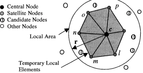
Let us see an example as shown in Fig.l, when we are considering the node "c" as a central node. Here the two
dimensional case is used to demonstrate the concept of Free Mesh Method simply. First we collect candidate nodes around
the node "c" by using a circle of radius "r", of which the center is located at node "c". The candidate nodes around node "c"
are those within the circle. Next, for the group of candidate nodes and the node "c", local elements between satellite
nodes( 1, m, n, o, p . . . . ) and the node "c" can be made by one of some kinds of mesh generation algorithm. Then stiffness
matrix for local elements around node "c" can be made by the traditional way as in FEM, and can be added to
The global system equations can be obtained by repeating the above corresponding row of global stiffness matrix.
procedures, node by node independently.
• Central Node ® Satellite Nodes 0 Candidate Nodes 0 Other Nodes
Local Area
Temporary Local Elements
0
Oq
0
0
1(
For making local elements from a local node group of candidate nodes and a central node, a method was proposed at
the beginning of the Free Mesh Method for the two-dimensional case [6]. The method is to make quadrilateral from
satellite nodes and the central node, then to divide it to 2 triangle by comparing the lengths of 2 diagonal lines of the
quadrilateral. With more generality, Delaunay tessellation can be adopted for both two- and three-dimensional cases [ 10].
T H R E E D I M E N S I O N A L F M M U S I N G D E L A U N A Y T E S S E L L A T I O N
Local Delaunay Tessellation
Delaunay tessellation is originally a concept in geometry, which is a method to divide a convex domain defined by a
set of points, to tetrahedrons without any opening, in the three dimensional case. The tetrahedrons divided by Delaunay
tessellation have a nature that, for a tetrahedron, there exists no other node within its circumscribed sphere, except the
vertices. The two and three dimensional Delaunay tessellation has been adopted as mesh generating algorithm in FEM, and
has become a almost developed one.
As a method to generate temporary elements for local domains in FMM, the three dimensional Delaunay tessellation
has been applied into FMM[ 10], and extension has been made to application to problem with complicated boundaries[ 11 ].
Here we applied such local Delaunay tessellation to the Mixed-FMM, with some improvements discussed as below.
Degeneration with 5 Nodes on a Same Sphere
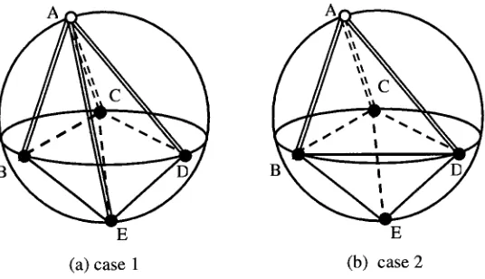
In the three dimensional Delaunay tessellation, when 5 points are on a same spherical surface, a degeneration
problem shown in Fig.2 will occur. As shown in Fig.2, both tessellation of case 1 and case 2 are possible to be made,
which means the result of Delaunay tessellation is not identical.
When generating global mesh over the whole domain by Delaunay tessellation, both case 1 and case 2 are acceptable
because they are equivalent to each other, so it will not affect much to the result analysis. But when generating local mesh
for FMM, if local mesh of case 1 shown as Fig.2(a) is generated for node "A" as central node, while local mesh of case 2
shown as Fig.2(b) is generated for node "E" as central node, the identification between local meshes over a same domain
losts, which will cause error.
To solve the above problem, we number the all nodes of the global domain, then add nodes by the order of the global
number when generating local mesh for each domain around every node as central node. Also, when an added node is on
the spherical surface of a tetrahedron, the tetrahedron must be modified. So the order of adding node will be identical, and
local mesh will also be identical for adjoining nodes when they are central nodes respectively.
A A
E E
(a) case 1 (b) case 2
Degeneration with 6 Nodes on a Same Sphere
For Delaunay tessellation of the two dimensional domain, when 5 nodes are on a circle, degeneration problem may
occur sometimes due to numerical error. For Delaunay tessellation of the three dimensional domain, when 6 nodes are on a
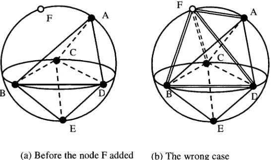
spherical surface, a similar degeneration problem may also occur due to numerical error, as shown in Fig.3. Considering
the case shown in Fig. 3(a), where the node "F" is added, after the tetrahedrons ABDC and BCDE have been generated,
while "A, B, C, D, E, F" are theoretically on a same spherical surface. Due to the numerical errors when calculating radius
of circumscribed sphere and the distance between the center of the sphere and the added node, it may result that the added
node "F" is out of the circumscribed sphere of tetrahedron ABDC. As a result, a new tetrahedron BCDE will be added,
while the tetrahedrons ABDC and BCDE remain, which results an overlapping between tetrahedrons ABDC and BCDF.
To solve such a degeneration problem, several methods are proposed [12], such as improving calculating accuracy,
postponing the processing of the node, moving the node slightly, calculating by integer, and a method shown below, which
we adopted for FMM. That is, when "r" is radius of the circumscribed sphere of a tetrahedron, and "d" is the distance
between the center of the sphere and the added node, the added node is judged to be in the circumscribed sphere only if the
following condition is satisfied:
r - d
~ £ (1)
Where, e is a tiny decimal which is set appropriately. This method can solve almost the degeneration problems of
this type pratically.
E E
(a) Before the node F added (b) The wrong case
Fig. 3 6-point Degeneration in 3-D Delaunay Tessellation
Degeneration with 4 Nodes on a Same Circle
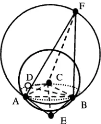
As an original degeneration problem of the three dimensional Delaunay tessellation, it is shown in Fig. 4 where 4
nodes of "A, B, C, D" are on a same circle. It means that, the node "D" is on the same plane where the triangle "ABC" is
located, and it is also on the circumscribed circle of the triangle "ABC". So the 2 tetrahedrons "ABCE" and "ABCF" which
both include the triangle "ABC" will have the added node "D" on their circumscribed spherical surfaces respectively.
Theoretically, because the triangle "ABC" is a common face of the 2 tetrahedrons "ABCE" and "ABCF", it will not be
added to the list of triangle, which will be combined with the added node to form tetrahedrons. But due to numerical errors
while out of another's. In such a case, the triangle "ABC" and the added node "D" will form a new tetrahedron, of which
volume is zero.
For this degeneration problem, the two tetrahedrons including a common triangle may have circumscribed spheres of
different radiuses. So the range of errors when calculating radiuses or distances will depend not only on the hardware and
compiler, but also on the radiuses. It results that a specific decimal o f " ~ " of above section can not solve this problem.
We proposed a method here to solve this problem as below. When generating the list of tetrahedron of which
circumscribed spheres include the added node, we calculate whether the added node is on the same plane of any face of all
the tetrahedrons. If the added node is on the same plane with one of a face of a tetrahedron, then another tetrahedron which
also includes the same face must be added to the list of tetrahedron of which circumscribed spheres include the added node.
It is an effective solve to this type of degeneration problem.
Fig. 4 4-point Degeneration in 3-D Delaunay Tessellation
F O R M U L A T I O N OF MIXED FREE MESH M E T H O D
Here we introduce a mixed formulation of elasticity which is based upon the Hu-Washizu's principle [13] to FMM.
The Hu-Washizu's principle states the stationary of the following functional:
-
o-f
f
f
O £2 g2 F l
(2)
where u =- f f on 1-',,, D is matrix of constitutive relation, b is body force, t is force vector, and S is derivative matrix
operator.
We approximate stress o , strain ~ and displacement u by their respective nodal value Crd, ~ d, Ud independently as
below:
O " - N a O " d
E - N e E d
u -- N u u d
(3)
where N o, N ~, and Nu are shape functions of stress, strain and displacement respectively. We use linear function for
A
C
O ] [ e d 0o
E l J a d
--
(4)where
A = ~ N:DN~dg2
(5)E - ~ N ~ B d g 2
(6)C - - ~ N : N , ~ d g 2
(7)If="
-N ubd£2+
f,'-
N = t d F
t
(8)
The equation system can be rewritten as following:
CO" d = - A £ d
6 7",E d = - E u d
Kud = f
(9)
where
/ ~ - E v ( C T A -l C ) - 1 E (~o)
m
As shown in Equation (10),
K
must be calculated after assembling all related global matrixes over whole analysis domain. Also calculation of the inverse of matrixes is needed. So the calculation cost will be too expensive. Here we use an iterative scheme [ 13] to solve such an equation system.First, one begins with following iterative equation about nodal displacement:
u n+l
- U a
n _ K - 1r
n (11)where n is number of iteration, and K is stiffness matrix of "standard" displacement method, r is residure vector which can be calculated by following equation:
r n -
E T
o" d - f n (12)After the displcaement is calculated, strain and stress can be calculated by following equations:
(O"; +'
) i - -(D•; +I
) i (14)Note here, for elasticity domain, stress can be calculated by constitutive equation, node by node. Using strain and stress, residure can be obtained to make the next iteration•
ALGORITHM OF MIXED FREE MESH METHOD
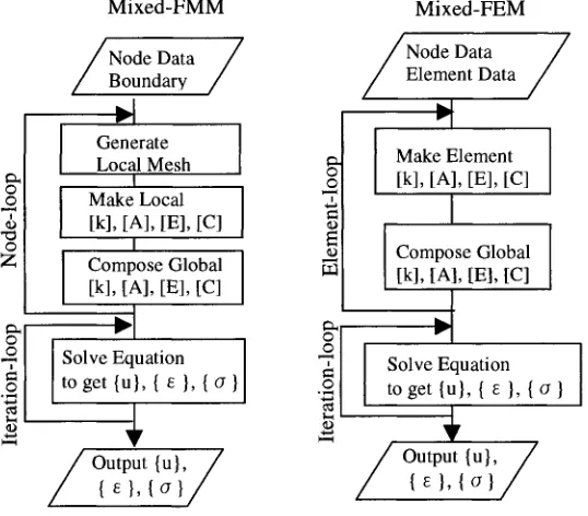
In Fig. 5 is shown the differences of algorithm between Mixed FMM and FEM using also mixed formulation( here called as Mixed-FEM).
As can be seen from Fig. 5, the input data needed by Mixed-FMM are only boundary data composed from triangle patches and coordinate data of nodes. Temporary local elements are generated internally in Mixed-FMM. On the other hand, as input data for Mixed-FEM, besides coordinate data of nodes, element-node connectivity data generated by pre- processor externally are also needed.
Also, when generating element matrix, in Mixed-FMM it can be done node-by-node independently, just after local mesh is generated, so it is easy to be parallelized.
O 6 O Z
il
Mixed-FMM Mixed-FEM
Node Data / Boundary iv- I Generate Local Mesh
I
Make Local [k], [A], [E], [C] Compose Global [k], [A], [El, [C]Solve Equation to get {u}, { e }, { cr }
I
Output
{u}, /
o o © r-r.l ID I,,-,,,4
Node Data / Element Data
Make Element [k], [A], [E], [C]
Compose Global [k], [A], [E], [C]
v I Solve Equation to get{u},{~},{cr}
/ou,put,u,,/
{~},{G}/
Fig. 5 Algorithm of The Mixed-FMM and Mixed-FEM
NUMERICAL EXAMPLE
Problem Definitions
For this example, we have used two analysis models with 160 nodes and 480 nodes, which are shown in Fig.7 and Fig.8 respectively.
Results of FMM and Mixed-FMM Using the Same Node Distribution
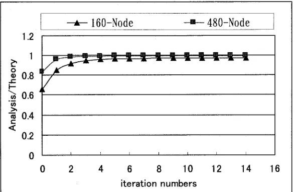
In this example, the number of iteration for mixed formulation is set to 14. In fig.9, the ratio of analysis results to the theoretical value for vertical displacement at the free tip is shown, for every iteration by using both 160-node model and 480-node model.
' ++~+i++++ii]+:"++++"--:++++++
Y
0.2 m ~ I tl ,,i'" / / 1.0m
L..]
x ~-"
~ F
Fig. 6 Cantilever Beam under Bending
/ , ~ ,
. , . : ,. , , , , . ' . ++,.,.]\.,,,- + ,, - , , _ , _ . _ \ _- ._.},,
\ / / ~ + • + • • • . . . . , . . . . ~ \ - /
Fig. 7 1 6 0 - N o d e FMM Model
. ; ~. ,. ,...+... + , . . . , . - - ~ . % ~ ; .~ ,~¢~.
-~.- ~ , , . ' . . . . ' ' , * - , ' - ' . . . . - . . . , , ' . ' . . , ~ ; . . " 1
• ".' , ; , l , • • . ' • •
• o l • • + D o + ~ + • e • • e 4~ I akin'
~ . . C . . .
¢ ++ + . . . ' . , . . - < . , - ' . " . . - - . . : ~ - " : ' t
~ 4 i ~ _ 4t' _ I . I I _ l l 4 1 ' _ I _ I _ 6 _ l " t ' + I . I 6 1 1 'tJ _4t , g l I ~l...,,Jl'
i f
Fig. 8 4 8 0 - - N o d e FMM Model
error of FMM is 34.37%, while the error of Mixed-FMM is reduced to 2.85%. In table. 2, which is result of using 480-
node model, the error of FMM still remains at a high value of 16.6%, while the error of Mixed-FMM is reduced
dramatically to 0.25%. For both models, Mixed-FMM showed a great improvement of accuracy compared with
displacement-based FMM.
-"
160-Node
... --- ... 4 8 0 - N o d e1.2
1 ... . ... 1 .... ! _
1
80.8
t -
~o 0.6 .m
> ,
"~ ¢. 0.4
<
0 . 2
I I t I I I I
0 2 4 6 8 10 12 14 16
iteration numbers
Fig. 9 Vertical Displacement at Free End v.s. Iteration Numbers
Table. 1 Vertical Displacement at Free End by 160-Node Model
I 160-Node FMM 160-Node Mixed-FMM Theoretical result
Uz -2.344 X 10⁻³m -3.470 X 10⁻³m -3.5714X 10³m
Error 34.37% 2.85%
Table. 2 Vertical Displacement at Free End by 480-Node Model
1 480-Node FMM 480-Node Mixed-FMM Theoretical result
Uz -2.977 X 10 -3 m -3.562 X 10 -3 m -3.5714 X 10 -3 m
Error 16.6% 0.25%
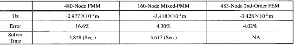
Results of F M M and Mixed F M M at the Same Number of D.O.F
In the formulation of Mixed-FMM described above, the number of degree of freedom(D.O.F) for each node is 9, which
is composed by 3 for displacement and 6 for strain. It is 3 times to that of displacement-based FMM. So the total D.O.F of
the 480-node model using FMM formulation is the same as the 160-node model using Mixed-FMM formulation.
In Table.3, the result by Mixed-FMM using 160-node model is compared with the result by displacement-based FMM
using 480-node model. For the former, the result at 4th iteration for mixed formulation is adopted. Also, the result of FEM
using a 483-node quadratic tetrahedral element model is shown in Table.3. "Solver Time" in Table.3 means the time
consumed to solve linear equation systems by the "conjugate gradient method", which for Mixed-FMM includes the times
According to Table.3, it can be seen that, with a same number of D.O.F., the Mixed-FMM with 4 iterations shows a great improvement of accuracy, compared to displacement-based FMM. And it should be noted that the improvement is achieved without increase of computer time. Also, the accuracy of Mixed-FMM with 4 iterations is almost the same as that of FEM using quadratic tetrahedral element.
Table. 3 Comparison between Displacement-Based FMM, Mixed-FMM with 4 Iterations and 2nd-Order FEM
Uz Error Solver
Time
II 480-Node FMM
-2.977 X 10 .3 m 16.6% 3.828 (Sec.)
160-Node Mixed-FMM -3.418 X 10⁻³m
4.30% 3.617 (Sec.)
483-Node 2nd-Order FEM -3.428 × 1 0 -3 m
4.02% NA
C O N C L U S I O N
Some degeneration problems when applying Delaunay tessellation to local mesh generating is discussed, and solves to these degeneration problems are proposed respectively. Then, to improve the accuracy of FMM, a mixed formulation in elasticity is applied to the three dimensional FMM. As a numerical example, stress analyses of a cantilever beam under concentrated load is performed, by using displacement-based FMM and Mixed FMM respectively. The results of the analyses are discussed, and a remarkable improvement of accuracy of the latter compared to that of the former is shown. Also, comparison with the result by FEM using second order tetrahedral element is done, and it is shown that the accuracy of both is almost the same.
REFERENCES
1. G.Yagawa and R.Shioya, "Parallel finite elements on a massively parallel computer with domain decomposition", Comput. Methods Appl. Mech. Engrg. 40 (1983)27-109
2. W.K.Liu, S. Jun and Y.F. Zhang, "Reproducing kernel particle methods", Int. J. Numer. Methods Fluids, 20(1995) 1081-1106
3. B. Nayroles, G. Touzot and P. Villon, "Generalizing the finite element method: Diffue approximation and diffuse elements", Comput. Mech. 10(1992) 307-318
4. T. Belytschko, Y.Y. Lu and L. Gu, "Element-free Galerkin methods", Int. J. Numer. Methods Engrg. 37(1994) 229- 256
5. P. Lancaster and K. Salkaushkas, "Surfaces generated by moving least squares methods", Math. Comput. 37(1981) 141-158
6. G.Yagawa, T.Yamada, "Free Mesh Method: A New Meshless Finite Element Method",
Int. J. Comp. Mech.,
18, 383- 386(1996)7. M.Shirazaki, G. Yagawa, "Large-scale parallel flow analysis based on free mesh method: a virtually meshless method",
Comput. Methods Appl. Mech. Engrg.,
174 (1999) 419-4318. G. Yagawa, M. Shirazaki, "Parallel computing for incompressible flow using a Nodal-Based method",
Computational
Mechanics,
23 (1999) 209-2179. K. Goto, G. Yagawa, T. Miyamura, "Two-dimensional Elasto-plastic Dynamic analysis Using the Free Mesh Method", Transactions of the Japan Society of Mechanical Engineers, Vol. 65, No. 639(1999-11), 2207-2211
10. G. Yagawa, T. Hosokawa, "Application of the Free Mesh Method with Delaunay Tessellation in a 3-Dimensional Problem", Transactions of the Japan Society of Mechanical Engineers, Vol. 63, No. 614(1997-10), 2251-2256 11. G. Yagawa, T. Hosokawa, " Application of the Free Mesh Method to a Three-Dimensional Complex Shape",
Transactions of the Japan Society of Mechanical Engineers, Vol. 64, No. 627(1998-11), 2741-2746 12. P.L.George, Automatic Mesh Generation, John Wiley & Sons(1991)
13. O.C. Zienkiewicz, R.L. Taylor, Finite Element Method, Vol. I, 4th Ed., McGRAW-HILL Book Company(1989)