Shape Reconstruction from Shadows and Reflections
Thesis by
Silvio Savarese
In Partial Fulfillment of the Requirements for the Degree of
Doctor of Philosophy
California Institute of Technology Pasadena, California
c
2005
Acknowledgements
I wish to thank my advisor, Pietro Perona. His advice and guidance during these years have made a sub-stantial difference in my work. I also wish to express my gratitude to Dr Fausto Berbardini, Professor Holly Rushmeier, Professor Gabriel Taubin, Dr Min Chen and Marco Andreetto for their close collaboration. I am grateful to Professor Jean Ponce, Professor Jerry Marsden, Professor Stefano Soatto, Dr Marzia Polito, Dr Matthew Cook, Dr Jean-Yves Bouguet for helpful feedback and many fruitful discussions. I would also like to thank the other members of my committee, Professors James Arvo, Demetri Psaltis, Shinsuke Shimojo and Jehoshua Bruck.
Abstract
Measuring automatically the shape of physical objects in order to obtain corresponding digital models has be-come a useful, often indispensable, tool in design, engineering, art conservation, computer graphics, medicine and science. Machine vision has proven to be more appealing than competing technologies. Ideally, we would like to be able to acquire digital models of generic objects by simply walking around the scene, while filming with a handheld camcorder. Thus, one of the main challenges in modern machine vision is to develop algo-rithms that: i) are inexpensive, fast and accurate; ii) can handle objects with arbitrary appearance properties and shape; and iii) need little or no user intervention.
In this thesis, we address both issues. In the first part, we present a novel 3D reconstruction technique which makes use of minimal and inexpensive equipment. We call this technique ”shadow carving”. We explore the information contained in the shadows that an object casts upon itself. An algorithm is provided that makes use of this information. The algorithm iteratively recovers an estimate of the object which i) approximates the object’s shape more and more closely; and ii) is provably an upper bound to the object’s shape. Shadow carving is the first technique to incorporate ”shadow” information in a multi-view shape recovery framework. We have implemented our approach in a simple table-top system and validated our algorithm by recovering the shape of real objects.
It is well known that vision-based 3D scanning systems handle specular or highly reflective surfaces only poorly. The cause of this deficiency is most likely not intrinsic, but rather due to our lack of understanding of the relevant cues. In the second part of this thesis, we focus on how to promote mirror reflections from ”noise” to ”signal”. We first present a geometrical and algebraic characterization of how a patch of the scene is mapped into an image by a mirror surface of given shape. We then develop solutions to the inverse problem of deriving surface shape from mirror reflections in a single image. We validate our theoretical results with both numerical simulations and experiments with real surfaces.
Contents
Acknowledgements iv
Abstract v
Table of Contents
1 Introduction 1
1.1 Toward an Ideal Visual System to Acquire Digital Models . . . 1
1.2 Shadow Carving: Combining Low Cost with Robust Shape Recovery . . . 2
1.3 Beyond Matte Surfaces . . . 4
1.4 Can We See the Shape of a Mirror? . . . 9
2 Shadow Carving 11 2.1 Introduction . . . 11
2.1.1 Chapter Organization . . . 12
2.2 Background . . . 13
2.3 Shadow Carving . . . 15
2.3.1 The Shadow Carving Theorem . . . 16
2.3.2 The Epipolar Slice Model . . . 17
2.3.3 Example . . . 18
2.3.4 The Shadow Decomposition . . . 20
2.3.5 The Atomic Shadow Case . . . 24
2.3.6 The Composite Shadow Case . . . 25
2.3.7 Effect of Errors in the Shadow Estimate . . . 27
2.4 A System for 3D Reconstruction from Silhouettes and Shadows. . . 28
2.4.1 Background: Shape from Silhouettes . . . 28
2.4.2 First Phase – Shape from Silhouettes . . . 30
2.4.3 Combining Approaches. . . 32
2.4.4 Second Phase – Shadow Carving . . . 32
2.5 Implementation . . . 34
2.5.1 Hardware Setup . . . 34
2.5.2 Software – Space carving . . . 36
2.5.3 Software – Shadow Carving . . . 37
2.5.4 Software – Post Processing of the Surface . . . 41
2.6 Experimental Results . . . 41
2.6.1 Experiments with Synthetic Objects . . . 41
2.6.2 Experiments with Real Objects . . . 46
2.6.3 Discussion . . . 50
3 Computational Analysis for 3D Reconstruction of Specular Surfaces 53
3.1 Introduction and Motivation . . . 53
3.1.1 Proposed Approach and Summary of the Results . . . 54
3.1.2 Previous Work and Our Contribution . . . 54
3.1.3 Chapter organization . . . 56
3.2 Problem Formulation . . . 57
3.2.1 Notation and Basic Geometry of Specular Reflections . . . 57
3.2.2 Reference System and Surface representation . . . 59
3.2.3 Differential Approach . . . 60
3.3 Direct Problem . . . 60
3.3.1 First Order Analysis . . . 61
3.3.1.1 First-order Derivative ofr(t) . . . 61
3.3.1.2 Relationship Betweenr˙andq˙ . . . 65
3.3.2 Second Order Analysis . . . 67
3.3.2.1 Second-Order Derivative ofr(t) . . . 67
3.3.2.2 Relationship Betweenr˙,¨randq¨ . . . 72
3.3.2.3 Relationship Betweenr˙,¨randκq . . . . 73
3.4 Properties of the Reflection Mapping . . . 75
3.4.1 Geometrical Configurations . . . 75
3.4.1.1 Singular Configurations . . . 76
3.4.1.2 Degenerate Configurations . . . 77
3.4.2 The Rank Theorem . . . 79
3.4.3 The Generalized Rank Theorem for Arbitrary Tangent Directions . . . 82
3.5 The Inverse Problem . . . 84
3.5.1 Inverse Problem . . . 84
3.5.2 Parameter Reduction . . . 86
3.5.3 Image Measurements: Curve Orientations . . . 86
3.5.3.1 Recovering the First-Order Parameters . . . 87
3.5.3.2 Reconstruction Algorithm . . . 88
3.5.3.3 Numerical Simulations and Discussion . . . 88
3.5.3.4 Recovering the Second-Order Parameters: the Second-Order Ambiguity . 89 3.5.3.5 Recovering the Second-Order Parameters: Two Special Cases . . . 91
3.5.3.6 Recovering the Second-Order Parameters: General Case . . . 92
3.5.3.7 Recovering the Third-Order Parameters . . . 97
3.5.4 Image Measurement: Orientations + Local Scale . . . 97
3.5.4.1 Recovering the First- and Second-Order Parameters . . . 98
3.5.4.2 Recovering the Third-Order Parameters . . . 99
3.5.4.3 Reconstruction Procedure . . . 102
3.5.4.4 Reconstruction Error . . . 104
3.5.4.5 Generalized Mapping . . . 105
3.6 Experiments . . . 106
3.6.1 Results with Algorithm A1 - Measurement of Orientations . . . 107
3.6.2 Results with Measurement of Orientations and Scale . . . 109
3.7 Conclusions and Future Work . . . 110
4 Human Perception of Specular surfaces 116 4.1 Introduction . . . 116
4.1.1 Chapter Organization . . . 118
4.2 Methods . . . 119
4.3 Results . . . 120
4.4 Analysis . . . 122
4.5 Conclusions . . . 123
Chapter 1
Introduction
1.1
Toward an Ideal Visual System to Acquire Digital Models
For the last thirty years, the possibility of capturing digital representations of physical objects has been receiv-ing an enormous amount of attention in information technology research. Contrary to physical models, digital models can be easily stored, retrieved in databases, edited in computer-aided-design (CAD) based software, transmitted and received through digital communication systems, used as templates for reverse engineering, displayed and analyzed at different resolution, and more. As a result, digital models are used in many appli-cations. Perhaps the most important ones are archaeology, education, medicine, entertainment, virtual reality, computer graphics, design and prototyping of industrial components, e-commerce, and robotics.
There exist several different ways of capturing digital models. Machine vision has proven to be more attractive than many competing technologies. For instance, acquiring models from visual inputs (such as images) is, by far, more convenient and faster than making use of touch probes. Ideally, one would like to be able to acquire digital models by simply walking around the scene, while filming with a handheld camcorder. This possibility has boosted vision research enormously and several techniques have been proposed. These techniques mainly differ in: i) the type of visual cues being used for shape recovery (texture, shading, contours systems); ii) the number of observers (monocular, stereo or multi-view stereo); and iii) the possibility of projecting ”active cues” such as structured lighting on the object surface (laser stripes, structured lighting patterns, shadows, etc).
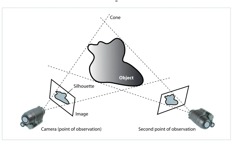
Camera (point of observation) Image Silhouette
Object
Cone
Second point of observation
Figure 1.1: A simple approach to recover the shape of an object: shape from contours (or silhouettes). The silhouette and the point of observation for each view form a cone containing the object. The intersection of multiple cones is an estimate of object shape. Shape from contour techniques, however, fail at recovering object concavities.
far from having an ”ideal” vision system. Ultimately, one would like to be able to recover digital models quickly, accurately, at low cost, and, with minimal human intervention.
With that specific goal in mind, we developed a novel approach for 3D reconstruction of objects. We call this approach ”shadow carving”.
1.2
Shadow Carving: Combining Low Cost with Robust Shape
Re-covery
Shadow Carving is the first technique that incorporates ”shadow” information in a shape-from-contour re-construction framework.
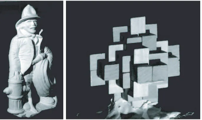
Figure 1.2: Objects concavities may be revealed by the presence of shadows that the object casts upon itself.
been proposed and subsequent research has improved on the efficiency of this approach. Because they are robust and conservative, techniques similar to Martin and Aggrawal’s original method have found success in low-end commercial scanners. These approaches, however, are quite inaccurate when the object presents concavities, the reason being that concavities cannot be modelled using contours. As a result, severe artifacts are often generated in the final reconstruction of the model.
Computing shape from shadows – or shape from darkness – has also been studied for many years. Shafer and Kanade [63] established fundamental constraints that can be placed on the orientation of surfaces, based on the observation of the shadows one casts on another. Since then, several methods for estimating shape from shadows have been presented. All of these methods, however, rely on accurate detection of the beginning and ends of shadow regions. This is particularly problematic for attached shadows that are the end of a gradual transition of light to dark. Furthermore, existing shape from shadow methods essentially recover terrains with some hole estimates, rather than complete three dimensional objects.
A major advantage, however, is that shape from shadow methods allow the reconstruction of the shape in concavities. Such concavities would not appear in any silhouette of the object (see Fig. 1.2).
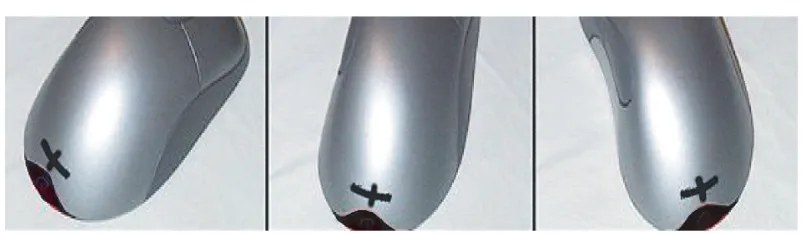
Figure 1.3: For specular objects, the brightness measured on the object’s surface is not invariant with respect to the viewer’s position. Rather, it depends on the position of both viewer and light source. Notice that the relative position between the highlight and the black cross changes as the viewer changes position.
object’s contours. Then, we use the information provided by the object’s shadows within an image. We make use of these cues to ”carve” away pieces of the current surface estimate. We obtain a new estimate which is a closer approximation of the actual surface of the object. By adding images taken under different lighting, one may iterate this process. We proved that the algorithm generates a sequence of conservative estimates, and that the information provided by each new image is used efficiently.
Coupling ”shadows” and ”contours” information allow to combine robustness with low cost and good accuracy. The issue of low cost is worked out in that we propose a system that uses a commodity digital camera and controlled lighting systems composed of inexpensive lamps. Additionally, since our method relies on substantial variations in the intensities in acquired images, it avoids requiring the user to set parameters and hence, minimizes the user’s intervention. Finally, since our technique progressively improves conservative estimates of surface shape, it avoids having an unstable method in which small errors accumulate and severely impact the final result.
We describe shadow carving in more detail in Chapter 2.
1.3
Beyond Matte Surfaces
Algorithms based on feature-matching (stereo, structure from motion, voxel coloring) are based on the assumption that small surface features can be identified in images taken from different positions. Similarly, photometric stereo and shape from shading algorithms assume that the pixel brightness depends only on the position of the light source relative to the surface. Both hypotheses are not true for specular surfaces. In active lighting techniques, stripes or patterns of light are projected on the object surface from a laser or LCD projector. Unfortunately, shiny surfaces reflect most light along the specular direction, and therefore the signal observed by the imaging device might be either very low or measured in the wrong position. Techniques based on occluding contours require segmenting the object against the background. This task may become very hard as grazing-angle reflections of the surrounding scene make such boundaries ‘melt’ visually with the background. Shape-from-texture techniques exploit intrinsic features (albedo) of the diffuse components of the reflectance function. In order for these methods to work, it is necessary to rule out texture features due to reflections of the surrounding scene and only consider those due to the diffuse component.
Yet, the ability to recover the shape of highly specular surfaces is valuable in many applications such as: • Industrial metrology: measurements of mechanical parts are needed for prototyping and quality control
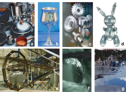
of industrial objects. Most objects of interest have highly reflective and polished surfaces (see Fig. 1.4, panel c).
• Diagnostic and control of space structures: large space structures are built of extremely light-weight components and thus, are highly susceptible to complex oscillations, as well to damage from debris. These surfaces are often metallic and highly reflective. On-line measurement of surface deformation is useful for stabilization and control. Diagnosis of impact damage is equally useful (see Fig. 1.4, panel e).
• Medical imaging: digital models need to be captured and displayed for diagnosis as well for on-line control of surgical procedures. Moist anatomical parts like the cornea of the eye and tissues that are visible endoscopically are highly reflective (see Fig. 1.4, panel f).
• Remote sensing of the surface of water: geophysical forces acting on water (i.e., wind, currents) may be studied through measurements of the shape of the surface (see Fig. 1.4, panel g).
• E-commerce: the possibility of viewing 3D interactive models of products over the web is appealing to customers. Many consumer products have highly glossy surfaces (see Fig. 1.4, panel a).
a
b
c
d
e
f
g
Figure 1.4: Applications. Panel a: E-commerce. Panel b: digital archival of heritage objects. Panel c: industrial metrology. Panel d: digital archival of art. Jeff Koons: Rabbit, 1986 stainless steel 41 x 19 x 12 inches -courtesy of The Broad Art Foundation. Panel e: diagnostic and control of space structures. Hexapod Structure - Tennessee State University / NASA Langley, courtesy of Dr. Gary A. Fleming. Panel f: medical imaging. Panel g: Remote sensing of the surface of water.
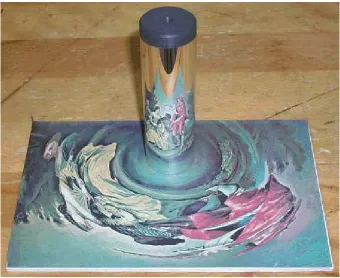
For shiny objects, one additional cue may be precisely the reflection of the environment. In fact, a curved mirrored surface produces distorted images of the surrounding world. For example, the image of a straight line reflected by a curved mirror is, in general, a curve. It is clear that such distortions are systematically related to the shape of the surface. Is it possible to invert this map and recover the shape of the mirror from the images it reflects? The problem is clearly highly under-constrained. By opportune manipulations of the surrounding world, we may produce almost any image from any curved mirror surface. This property is well known by artists, as illustrated by the anamorphic images that were popular during the Renaissance (see Fig. 1.5).
Figure 1.5: The problem of recovering the shape of a mirror from its specular reflections is highly under-constrained. By opportune manipulations of the surrounding world we may produce almost any image from any curved mirror surface. Examples are anamorphic images as shown in this figure. Anamorphic images are drawn by knowing the relationship between the proportions of a real object to the proportions of its reflected image on a mirror surface of known curvature. Once an anamorphic image is drawn, it can be restored to its corrected proportions by reflecting it in the mirror surface. Typical surfaces used for anamorphic images are cones and cylinders.
light source, specular highlights do not contain enough information to recover the shape univocally. Thus, the relevance and the use of additional geometrical constraints (multiple cameras and moving observer) were explored [36, 4, 84, 49, 82] . Often these efforts led to techniques requiring dedicated and expensive hardware equipment.
Figure 1.6: The task of recovering the shape of a mirror from its specular reflections may be very hard for the human visual system. The figure in the left panel shows a specular surface with a concavity in the center. It is quite difficult to perceive the actual shape of the concavity. Notice that object contours give very little information about the shape of the concavity. The figure in the right panel, shows the same specular surface seen from a different side. The geometry of the concavity becomes now much more clear. In this case, contours seem to play an important role in the perception of the shape, so we are interested in addressing the question: to what extent can the human visual system use specular reflections to perceive the shape of specular surfaces when other visual cues (such as shading, texture, contours) are absent?
different condition of the illuminant are required.
We propose a novel approach where the local shape of an unknown smooth specular surface can be recovered by observing its deforming behavior acting on the reflection of the scene. Our assumptions are that: i) the mirror surface is smooth; and ii) the reflected scene has known structure and position. Under these assumptions, we first describe a geometrical and algebraic characterization of how a patch of the scene is mapped into an image by a mirror surface. Then, we investigate the inverse problem and give necessary and sufficient conditions for recovering the local shape of the surface. Specifically, we prove that if the environment is composed of a planar patch of points or intersecting lines, then at any point the local shape can be recovered up to the third derivative.
Our technique differs and improves previous work in that it allows local shape reconstruction from a single image; it does not require prior assumption on object position or shape; it necessitates minimal and inexpensive hardware (one camera and a calibrated scene pattern only); local shape can be recovered in closed for solution; and the analysis is local and differential rather than global and algebraic.
1.4
Can We See the Shape of a Mirror?
One important consequence of our computational analysis is that necessary and sufficient conditions for recovering the local shape of mirror surfaces are provided. In other words, the local shape of a mirror surface reflecting a scene can be recovered only if a certain amount of knowledge about that scene is available. Our computational study tells us precisely what this ”amount” is.
What happens, then, if the surrounding world is unknown? The problem is under-constrained and many solutions are possible. This observation leads naturally to the question: how do humans cope with the problem of perception of the shape of specular surfaces, given that most of time, we do not have the exact geometrical information about the world? An answer to this question would be of great value. The study of human vision can help us understand what cues may be used and which algorithms may be feasible, and ultimately guide our analytical efforts in the most productive direction.
While the perception of shape from a number of other visual cues (shading, texture, motion, stereo-scopic disparity) has been extensively discussed in the human vision literature, surprisingly little is known to what extent the reflection of the environment off a specular surface may carry useful information for shape perception. The available knowledge is limited to the work by Beck, Koenderink and other re-searchers [36, 1, 73, 48]. Blake [5] showed that the human visual system successfully estimates shape and quality of a shiny object when the highlights are viewed stereoscopically. Recently, Fleming and collabora-tors [21] found in their experiments that the shape of mirror surfaces is readily perceived by human subjects. They explain their findings by noticing that specular reflections exhibit a different pattern of compression than surface texture. This feature would allow the human visual system to discriminate between these two cases and the pattern of compression would represent a cue for shape from specularities.
Through Chapter 4 of this thesis, we study this problem psychophysically and address the following questions: i) to what extent the human visual system can use specular reflections in isolation, namely, when other visual cues (such as shading, texture, motion, stereoscopic disparity) are absents ; ii) what are the underlying computational strategies for this task?
Chapter 2
Shadow Carving
2.1
Introduction
A number of cues, such as stereoscopic disparity, texture gradient, contours, shading and shadows, have been shown to carry valuable information on surface shape, and have been used in several methods for 3D reconstruction of objects and scenes. Techniques based on shadows have the advantage that they do not rely on correspondences, on a model of the surface reflectance characteristics, and they may be implemented using inexpensive lighting and/or imaging equipment. Past methods to recover shape from shadows, however, have proven to be sensitive to errors in estimating shadow boundaries. Additionally, their are mostly restricted to objects having a bas-relief structure.
We propose a novel 3D reconstruction method for using shadows that overcomes previous limitations. We assume that we have, as a starting point, a conservative estimate of object shape; that is, the volume enclosed by the surface estimate completely contains the physical object. We analyze images of the object illuminated with known light sources taken from known camera locations. We assume that we are able to obtain a conservative estimation of the object’s shadows - that is, we are able to identify image areas that we are certain to be in shadow region, and do not attempt to find exact shadow boundaries. We do not make assumptions about the surface topology (multi-part objects and occlusions are allowed), although any tangent plane discontinuities over the objects surface are supposed to be detected. Our basic idea is that we compare observed shadows to those expected as if the conservative estimate were correct and adjust the current shape to resolve contradictions between the captured images and the current shape estimate. In this process, we incrementally remove (carve out) in a conservative way volume from the current object estimate in order to reduce the inconsistencies. Thus, a closer objects shape estimate is computed at each step. We call this novel procedure shadow carving. We provide a proof that the carving process is always conservative.
robust with respect to the classification of shadow regions; ii) it gives the possibility of recovering objects in the round (rather than just bas-reliefs).
Our motivation for pursuing this work relies in applications where the user often has a very limited bud-get, and is primarily concerned with visually, rather than metrically, accurate representations. Furthermore, because users are often not technically-trained, the scanning and modeling systems must be robust and require minimal user intervention.
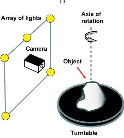
We validate our theoretical results by implementing a scanning system based on shape from silhouettes and shape from shadows. First, the silhouettes are used to recover an conservative estimate of the object shape. Then, a series of images of the object lit by an array of light sources are recorded with a setup shown schematically in Fig. 2.1. Such images are examined and the shadows that the object casts on itself are detected. The current shape estimate is then refined by the shadow carving procedure. Eventually, the improved estimate of shape can be further refined by methods that work well locally, such as photometric stereo [29].
Our system is designed to be inexpensive as other recently proposed schemes [53, 9]. It uses a com-modity digital camera and controlled lighting systems composed of inexpensive lamps. Additionally, since our method relies on substantial variations in the intensities in acquired images, it does not requires precise tuning, hence it minimizes the user intervention. Finally, since our technique progressively improves conser-vative estimates of surface shape, it prevents small errors from accumulating and severely deteriorating the final results.
2.1.1
Chapter Organization
Array of lights
Camera
Turntable Object
Axis of rotation
Figure 2.1: Setup for shape from self-shadowing: Using each of several lights in turn, and a camera in front, allows multiple sets of shadow data to be obtained for each object position.
2.2
Background
Computing shape from shadows – or shape from darkness – has a long history. Shafer and Kanade [63] established fundamental constraints that can be placed on the orientation of surfaces, based on the observation of the shadows one casts on another. Hambrick et al. [26] developed a method for labelling shadow boundaries that enables inferences about object shape. Since then, several methods for estimating shape from shadows have been presented. Because we aim at designing a 3D scanner, we focus on reconstruction schemes where the light source position is known, rather than the case of unknown light source direction (e.g., [37]). Also, we limit our analysis to methods using self-shadows (i.e., shadows cast by the object upon itself) rather than shadows cast by external devices as in [9]. Hatzitheodorou and Kender [27] presented a method for computing a surface contour formed by a slice through an object illuminated by a directional light source casting sharp shadows. Assuming that the contour is defined by a smooth function – and that the beginning and end of each shadow region can be found reliably – each pair of points bounding a shadow region yields an estimate of the contour slope at the start of the shadow region, and the difference in height between the two points as shown in Fig. 2.2. The information for shadows from multiple light source positions is used to obtain an interpolating spline that is consistent with all the observed data points.
f(x)
θ
light
xe xb
Figure 2.2: Shape from Shadows: For terrain surfacesf(x)and a known light source directionθ, f0(x b) =
tanθ, andf(xb)−f(xe) = f0(xb)(xe−xb). Using data for many anglesθan estimate of the continuous functionf(x)can be made.
the third coordinate being the angle of the light source to the reference surface, and the volume recording whether the reference surface was in shadow for that angle. A slice through this volume is referred to as a
shadowgram. Similar to Hatzitheodorou and Kender, by identifying beginning and ending shadow points for
each light position, the height difference between the points can be computed. Also, by observing the change in shadow location for two light source positions, the height between the start of the shadow at one position relative to the other can be found by integration. As long as shadow beginnings and endings can reliably be detected, the top surface of the object can be recovered as a height field. Furthermore, by detecting splits in the shadowgram (i.e., positions that have more than one change from shadowed to unshadowed), holes in the surface below the top surface can be partially recovered.
Langer et al. [39] extend the method of Raviv et al. for computing holes beneath the recovered height field description of the top surface for two dimensions. They begin with the recovered height field, an NxN discretization of the two dimensional space, and the captured shadowgram. Cells in this discretization are occupied if they are in the current surface description. Their algorithm steps through the cells and updates them to unoccupied if a light ray would have to pass through the cell to produce a lit area in the captured shadowgram.
Daum and Dudek [16] subsequently developed a method for recovering the surface for light trajectories that are not a single arc. The estimated height field description is in the form of an upper bound and lower bound on the depth of each point. The upper and lower bounds are progressively updated from the information obtained from each light source position.
that use gradients derived from the estimate of the start of attached shadows are particularly prone to er-ror. Yang [79] considers the problem of shape from shadows with erer-ror. He presents a modified form of Hatzitheodorou and Kender approach, in which linear programming is used to eliminate inconsistencies in the shadow data used to estimate the surface. While the consistency check does not guarantee any bounds on the surface estimate, it does guarantee that the method will converge. He shows that the check for in-consistences is NP-complete. While more robust than Hatzitheodorou and Kender’s method when applied to imperfect data, Yang’s technique is still restricted to 2.5D terrains. Finally, Yu and Chang [80] give a new graph-based representation for shadow constraints.
Our method does not require a restriction to 2.5D terrains. Rather, it allows a fully 3D reconstruction of the object. Additionally, we do not rely on knowing the boundaries of shadow regions to compute surface shape. Similar to Yangs approach, we use the idea of consistency to avoid misinterpreting data. However, rather than comparing multiple shadow regions for consistency, we check that observed shadow regions are consistent with our current surface estimate.
Our proposed approach - shadow carving - is similar in spirit to the space carving approach of Kutulakos and Seitz [38]. Our approach differs from [38] in that we consider consistency between a camera and light views, rather than multiple camera views. Consistency can be tested robustly by detecting shadows, without requiring the hypothesis of Lambertian surface. We begin with a conservative surface definition, rather than a discretized volume. Inconsistent regions can be carved out by moving surface points at the resolution of the captured images, rather than being limited to a set of fixed resolution voxels. Most importantly, we provide a proof of correctness that well defined portions of volume can be removed in a conservative manner from the current object estimate, instead of iteratively removing single voxels until all the inconsistencies are solved.
This chapter gathers our own previous work [61, 60] and presents an extended experimental analysis in that: i) performance of the method with different configurations of lights and camera positions is tested; ii) accuracy of the reconstruction due to errors in the shadow estimates is assessed; iii) throughout experiments with real objects are shown.
2.3
Shadow Carving
Oc = camera
Inconsistent
shadow L = light
Object R
Shadow Shadow
volume Vo
Carvable volume VC
Light volume VL
Conservative estimate of the object R^
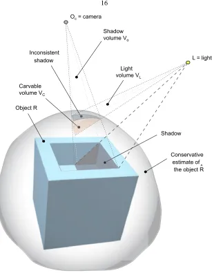
Figure 2.3: Example of shadow carving in 3D.
2.3.1
The Shadow Carving Theorem
Consider an object in 3-D space and a point light sourceLilluminating it. See Fig. 2.3. One or more shadows are cast over the object by parts of the object itself. The scene is observed by a pin-hole camera whose center is located inOc. Let us introduce the following definitions:
Definition 2.3.1 A conservative object estimate is any volumeRˆthat contains the objectR.
Definition 2.3.2 The shadow volumeVo is the set of lines through the center of the camera projectionOc
and all of the visible points of the object’s surface that are in shadow.
Definition 2.3.3 The inconsistent shadow is the portion of the surface of the conservative object estimate
Definition 2.3.4 The light volume VL is the set of lines through the light sourceL and the points of the
inconsistent shadow. We denote the dependency ofVLon the particular choice ofRˆbyVL( ˆR).
Definition 2.3.5 The carvable volumeVC( ˆR)isVo∩VL( ˆR)∩R, whereˆ Rˆis a conservative object estimate.
Theorem 2.3.1 If the object surface is smooth,RˆminusVC( ˆR)is a conservative object estimate.
Notice that all the quantities (i.e.,L,Oc,Rˆand the image points of the object’s surface that are in shadow) are available either from calibration or from measurements in the image plane. Therefore theorem 2.3.1 suggests a procedure to estimate the object incrementally: i) start from a conservative object estimate; ii) measure in the image plane all of the visible points of the object’s surface that are in shadow and compute the shadow volume; iii) compute the corresponding inconsistent shadows; iv) compute the corresponding light volume; v) intersect the conservative object estimate, the shadow volume and the light volume and calculate the carvable volume; vi) remove the carvable volume from the conservative object estimate to obtain an new object estimate. Theorem 2.3.1 guarantees that the new object estimate is still a conservative object estimate. The process can be iterated by considering a new light source or by viewing the object from a different vantage point. This procedure will be developed in details in section 2.4.
As we shall see in section 2.3.4, the theorem still holds if there are errors in detecting the visible points of the object’s surface that are in shadow. These errors, however, must be conservative; namely, a piece of shadow can mislabeled as non-shadow, but a non-shadow cannot be mislabeled as a shadow.
2.3.2
The Epipolar Slice Model
In order to prove Theorem 2.3.1 we examine the problem in an appropriately chosen 2-D slice of the 3-D space, the epipolar slice. As we shall discuss in more details in section 2.3.6, the results that we prove for a given slice hold in general and do not depend on the specific choice of the slice. Thus, the extension to the 3-D case is immediate by observing that the epipolar slice can sweep the entire object’s volume.
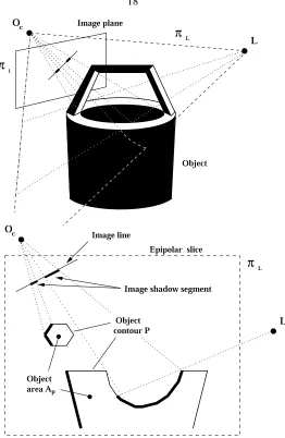
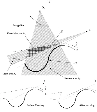
Consider the family of planes ΠL passing throughOc andL (see Fig. 2.4). Each planeπL ∈ ΠL, intersects the image planeπiand the object. In other words, eachπLdefines an epipolar slice of 3-D space. For each slice, we have the image line (i.e., the intersection ofπiwithπL), the image shadow segment (i.e., the intersection of the estimated image shadow withπL), the object contourP (i.e., the intersection of the object’s surface with πL) and the conservative object contourPˆ(i.e., the intersection of the conservative surface estimation withπL). We can also have the object areaAP (that is, the area bound byP) and the
Object area Ap
Image line Image plane
Oc
π
Lπ
iOc
π
LL Image shadow segment
Epipolar slice
L
Object
Object contour P
Figure 2.4: Top: An object in 3-D space and a point light sourceLilluminating it. The scene is observed by a camera whose center is located inOcand whose image plane is calledπi. Bottom: The planeπL defines an epipolar slice of 3-D space.
2.3.3
Example
Fig. 2.5 shows an example of shadow carving in the epipolar slice model. The shadow¯sis cast by the the object contourP over itself. sis the image ofs¯. The shadow areaAois the set of lines throughOcand all of the point alongs. The portion ofPˆthat is visible from the camera and the light, and intersectsAois the
inconsistent shadowsˆ. This shadow is called inconsistent because it is visible from the light sourceL. Thus, the conservative estimatePˆhas to be re-adjusted in order to explain this inconsistency. The light areaAL is the set of lines throughLand all of the points onˆsthat are visible fromL. Finally,Ao∩AL∩APˆgives
P ^
Light area A L
Carvable area Ac
P ^
P
L
Before Carving
P ^
P
L
After carving Shadow area Ao
L ^
P s
s s
O c
Image line
Figure 2.5: Example of shadow carving.
is consistent with the observed shadowsand with the light source position. Thus, no additional carving is required. Finally, notice thatAC can be removed in one shot rather than by means of an iterative process as in [38].
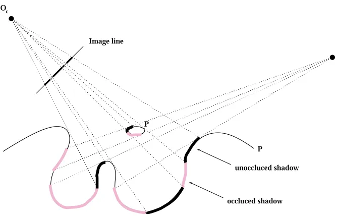
Many questions arise and we may wonder what happens if i) the topology of P is more complex; ii) the shadow is occluded by other object parts; iii) multiple shadows are imaged by the camera; iv) the object surface contains low-albedo regions that do not allow a correct or complete estimate of the shadows. Can we still define a carvable area? Can we guarantee that the carvable area is always outside the object (i.e., the new estimate is still conservative)?
Oc
P
L
P
unoccluced shadow
occluced shadow Image line
Figure 2.6: Example of occluded and unoccluded shadows.
smoothness of the object surface is required and is discussed at the end of Section 2.3.4.
2.3.4
The Shadow Decomposition
Let us consider an epipolar slice of a 3-D object. In general, the object’s contourP on the epipolar slice might comprise more than one separate contour components. For instance, the body of the bucket in Fig. 2.4 produces the contourP1and the handle produces the contourP2.
Given a point light sourceL, some portions of the object contour will be visible from the light source, whereas other portions will not.
Definition 2.3.6 A shadow is a portion of contour that is not visible from the light source.
Thus, depending on the object’s topology and the light source position, there will be a certain shadow distri-bution.
In general, some portions of a given shadow might be occluded from the camera view by other parts of the object. A portion of shadow which is visible from the camera (i.e from the center of projection) is called
unoccluded. Fig. 2.6 shows examples of unoccluded shadows: the unoccluded shadows are indicated with the
bold black lines; the occluded portions of shadow are indicated with bold pink lines. It is clear that whether a shadow is occluded or not only depends upon the contour topology and the camera position.
P P
L
undetectable regions
detectable shadow
detectable shadow undetectable region
Figure 2.7: Example of detectable shadows.
is labeled as shadow is indeed a shadow. See section 2.4.4 for details. Thus, a portion of contour is called
undetectable if, according to the shadow detection technique, it cannot be classified either as a shadow or as
not a shadow. We define detectable as a shadow which does not lie within an undetectable portion of contour. Fig. 2.7 shows examples of detectable shadows and undetectable regions: the hatched areas are undetectable contour regions; the detectable shadows are indicated in bold black.
Definition 2.3.7 A maximal connected portion of shadow which is both unoccluded and detectable is called
atomic.
An atomic shadow is indicated with the symbol¯aand its corresponding perspective projection into the image line is indicated bya. We callaan atomic image shadow. As a result, any shadow¯sj can be de-composed into its atomic components¯aj,1,a¯j,2... ¯aj,k. See Fig. 2.8 for an example: the atomic shadows
(indicated in bold black) within¯s1 are¯a1,1,¯a1,2, ¯a1,3 anda¯1,4. The perspective projection of the atomic
shadows into the image line yields the atomic image shadowsa1,1,a1,2,a1,3anda1,4.
We assume that the shadow detection technique gives us an estimationeuof the perspective projection into the image line of the complete set of unoccluded shadows and an estimationedof the perspective projection of the complete set of detectable regions. The intersection ofeuwithedgives the estimated shadow distribution
Oc
1 e a 1,1 U a 1,3
2 2,1
a e 3 e 3
a 1,4 4 e U
2,1 a
1,4 a
a 1,3
a 1,2
a 1,1
L
U a 1,2 Ue
( )
U
Figure 2.8: Example of atomic shadows.
shadows. For instance, see Fig. 2.8. The estimated shadow componente3 corresponds to atomic image
shadowsa2,1anda1,3.
Lemma 2.3.1 If the object contour’s first order derivative is continuous (i.e., the object’s contour is smooth)
and if the shadow detection is conservative (i.e., a piece of shadow can be mislabeled as non-shadow, but a
non-shadow cannot be mislabeled as a shadow), an estimated shadow component is always a lower bound
estimation of either an atomic image shadow or the union of two or more atomic image shadows.
Proof The lemma just follows from the definitions.
An example is shown in Fig. 2.8: the estimated shadowewithin the image line can be decomposed into its estimated shadow componentse1,e2,e3ande4. In particular,e1 is a lower bound estimation ofa1,1. e3is a lower bound estimation of the union ofa1,3anda2,1. Notice thate3appears as a connected shadow
component, althougha1,3anda2,1are the images of atomic shadows generated over two different contours.
In the following we want to show that if the hypothesis of smoothness is removed, Lemma 2.3.1 is no longer verified. Let us consider the example depicted in Fig. 2.9. The surfaceP casts two shadows overP
−
1
a
− a
2 1
a
2
e a 2
1
e
O
c
L
?
P −
p
U
U
Figure 2.9: Contour with singular point.
cannot be in shadow. Furthermore,p¯is visible fromOc. Thus, the corresponding atomic image shadowsa1
anda2 do not constitute a connected component. However, if the edge is sharp enough, the camera might
not be able to resolvep¯, which will be estimated as being in shadow. The shadow decomposition fails; the estimated shadow component is no longer a lower bound conservative estimate ofa1anda2. In other words, a1anda2are estimated to be a unique connected component instead of two disconnected shadow components e1ande2. As a result, Lemma 2.3.1 does not necessarily hold when the contour smoothness hypothesis is
not verified.
We can remove the hypothesis of smoothness if we suppose that we have available a technique to identify points whose first order derivative is not continuous. We call such points singular and we label them as undetectable. Let us consider again the example of Fig. 2.9. Ifp¯can be identified as singular and therefore its imageplabeled as undetectable,a1anda2are no longer estimated as a unique shadow component, but as two
disconnected estimated shadows componentse1ande2. The shadow decomposition is again conservative and
Lemma 2.3.1 is verified. From now on, we assume either to deal with smooth contours or to have a technique to identify singular points so that we can use the property stated in Lemma 2.3.1.
A c
O c
^
e ^ v ^ U e
A l
− a
A o L P P ^ e = a
Figure 2.10: The atomic shadow case.
2.3.5
The Atomic Shadow Case
Let us consider an estimated shadow componenteand let us assume thateis exactly the atomic image shadow
a(see Fig. 2.10). We call¯athe corresponding atomic shadow over the object contour. LetAobe the area defined by the set of lines throughOcande.Aois the 2D slice of the shadow volumeVoin definition 2.3.2. The following lemma holds:
Lemma 2.3.2 Given an estimated shadow componente and the corresponding shadow areaAo, all the
points belonging toP and withinAoeither belong toa¯or are not visible fromOc. In particular, if there is a
pointp∈P and∈Aonot visible fromOc, there must exist at least one pointq∈a¯betweenpandOc.
Proof. The lemma follows from the definition of atomic shadow and Lemma 2.3.1.
In the following, we introduce the geometric quantities necessary to formally define the carvable area. LetPˆbe the current conservative contour estimation and leteˆ(light gray line in Fig. 2.10) be the projective transformation (centered inOc) ofeonto the conservative contourPˆclosest toOc1SincePˆis a conservative
1We define a segmentˆs(e.g., a portion of the conservative estimate of object contour) to be closer than another segments¯(e.g., a
estimation of the realP,eˆis closer toOc then¯a. Letvˆ(black line in Fig. 2.10) be the portion ofˆewhose points can be connected by a line segment toLwithout intersectingPˆ. Thus, any point∈ˆvmust be visible fromL.ˆvcorresponds to the inconsistent shadow in definition 2.3.3. LetAlbe the area defined by the family of lines passing throughLand any point alongvˆ.Alis the 2D slice of the volumeVLin definition 2.3.4.
Definition 2.3.8 We define the carvable areaAC as the area obtained by the intersection of the estimated
object area (bounded byPˆ),AlandAo.
The carvable area corresponds to the cross-hatched area in Fig. 2.10 and is the 2D slice of the volumeAC in definition 2.3.5. The key result in this section is stated in the following lemma:
Lemma 2.3.3 The carvable areaACdoes not intersect the real object contourP.
Proof. Suppose, by contradiction, that there is a portionq of the object contourP within AC. There are two possible cases: qis fully included within the atomic shadow¯a(case1);qis not fully included withina¯
(case2). Let us start with case1. It is easy to conclude that, sinceACis defined byˆv(which is fully visible fromL), there must exist at least one pointp∈q ⊆ ¯avisible fromL. The contradiction follows from the definition of shadow 2.3.6. Consider case2: letqp be a portion ofqnot included in¯a. Since¯ais atomic, by Lemma 2.3.2,qpmust eventually be occluded by a portion¯ap ofa¯. But sinceeˆis closer toOcthan¯a and sinceqp belongs toAC,¯apmust lie withinAC. Hence we can apply case1to¯apachieving again the
contradiction. The lemma is fully proved.
Lemma 2.3.4 The carvable areaACcannot completely lie within the object.
Proof. The lemma holds because, by definition,eˆis closer toOcthena¯.
Proposition 2.3.1 Any point within a carvable area cannot belong to the actual object area.
Proof. The proposition follows from Lemma 2.3.3 and 2.3.4.
2.3.6
The Composite Shadow Case
The composite shadow case arises when e is not necessarily attached to a single atomic shadow (e.g., Fig. 2.11). Let us assume thateis actually composed by the union ofJatomic image shadowsa1, a2, . . . aJ.
O c ^ P ^ P − a 2 a
A l 1
− a
1
A o
L P P 2 1 2 ^ ^ e e A l
2
U
e = a 1
Figure 2.11: The composite shadow case.
Lemma 2.3.5 Given an estimated shadow componenteand the correspondingAo, all the points belonging
toP and withinAo either belong to one of the atomic shadowsa¯1,¯a2, . . .¯aJ or they are not visible from
Oc. In particular, if there is a pointp∈Pand∈Aonot visible fromOc, there must exist at least one point
q∈ {¯a1,¯a2, . . .a¯J}betweenpandOc.
Proof. The lemma directly follows from the definitions of atomic shadows, Lemma 2.3.1 and the assumption
thateis a connected shadow component.
We can defineˆeas in the atomic case. The difference here is thatˆemay be decomposed intoKdifferent componentseˆ1. . .eˆK located in different positions withinAo, depending on the topology of Pˆ. For each
k, we can define ˆvk as the portion ofˆek whose points can be connected by a line segment toL without intersectingPˆ. Furthermore, for eachˆvkwe define a correspondingAlkas in the atomic case.
Finally:
Definition 2.3.9 We define the set of carvable areasAC1,AC2, . . . ACK attached to the estimated shadow
componenteas set of areas obtained by the intersection among the estimated object area (bounded by P),ˆ
Aoand the setAl1, Al2, . . . ...AlK.
object area.
Proof. The proposition follows from Lemma 2.3.5 and by modifying accordingly Lemma 2.3.3, Lemma 2.3.4
and the corresponding quantities.
Proposition 2.3.1 and Proposition 2.3.2 guarantee that points taken from any of the carvable areas, are always outside the real object area. The extension to the 3-D case is immediate by observing that: i) the epipolar slice can sweep the entire object’s volume; ii) the interplay of light and geometry that allows us to prove Proposition 2.3.1 and Proposition 2.3.2 take place within each slice and is independent of the other slices. Thus, Theorem 2.3.1 is fully proven.
Notice that Theorem 2.3.1 holds under the hypothesis of Lemma 2.3.1: i) the actual object’s contour is smooth (or a technique is available to identify points whose first order derivative is not continuous - see section 2.3.4); ii) the shadow detection technique is conservative - that is, a shadow may not be detected but whatever is labeled as shadow is indeed a shadow.
2.3.7
Effect of Errors in the Shadow Estimate
What happens when errors in the shadow estimation occur? We proved Proposition 2.3.1 with the assumption that an estimated shadow component is equivalent to an atomic image shadow (or the union of two or more atomic image shadows). In the presence of a conservative error in the shadow estimation, the estimated shadow component is always included in the atomic image shadow. Thus, the corresponding carvable areas will be a subset of those obtained from the full atomic shadow. In the limit case where no shadows are detected, no volume is removed from the object. As a result, we still perform a conservative carving. This property makes our approach robust with respect to conservative errors in identifying shadows. If a non-conservative error in the shadow estimation occurs, however, the estimated shadow components may not necessarily be included in the corresponding atomic image shadows. As a result, some carvable areas may be contained within the actual object’s boundaries. The shadow carving procedure is no longer conservative. In section 2.6, we will show an example of non conservative carving due to non conservative errors in the shadow estimate.
2.4
A System for 3D Reconstruction from Silhouettes and Shadows.
In this section, we present the design of a system for recovering shape from shadow carving. The system combines techniques of shape from silhouettes and shadow carving. We first briefly review techniques based on shape from silhouettes in Section 2.4.1. Then we present our implementation of shape from silhouettes. We describe a new hardware configuration that tackle the difficult problem of extracting the object image silhouette in Section 2.4.2. The outcome of shape from silhouettes is an initial conservative estimate of the object. We review hybrid approaches in Section 2.4.3 and show that the initial estimate can be refined by shadow carving in Section 2.4.4.
2.4.1
Background: Shape from Silhouettes
The approach of shape from silhouettes−or shape from contours−has been used for many years. An early shape from silhouette method was presented by Martin and Aggarwal [47] and has subsequently been refined by many other researchers. The approach relies on the following idea. The silhouette of the object in the image plane and camera location for each view forms a cone containing the object. See Fig. 2.12. All space outside of this cone must be outside of the object, and the cone represents a conservative estimate of the object shape. By intersecting the cones formed from many different viewpoints, the estimate of object shape can be refined. Different techniques for computing the intersection of cones have been proposed. Martin and Aggarwal considered a volume containing the object and uniformly divided such volume in sub-volumes. For each view, each sub-volume−or voxel−is examined to see if it is outside of the solid formed by the silhouette and the view point. If it is outside, the voxel is excluded from further estimates of the object shape. Subsequent research has improved on the efficiency of this approach by alternative data structures [68] for storing the in/out status of voxels. Standard surface extraction methods such as Marching Cubes [43] can be used to compute the final triangle mesh surface. It is also possible to model the cones directly as space enclosed by polygonal surfaces and intersect the surfaces to refine the object estimate, similar to the method used by Reed and Allen to merge range images [52].
Object
Camera 2
Image 2
Camera 1 Image 1 Camera 3
Image 3
Figure 2.12: Shape from Silhouettes: The silhouette and camera location for each view forms a cone contain-ing the object. The intersection of multiple cones is a conservative estimate of object shape.
for a small change in orientation. The set of 3D points obtained from many views form a cloud that can be integrated into a single surface mesh. The method presented by Zheng has the advantage of the unobserved areas that have unmeasured concavities being identified automatically. It has the disadvantage that many more silhouettes are required to estimate the object shape. The method is also not as robust as the cone intersection methods, because reconstruction errors inherent in meshing noisy points may result in holes or gaps in the surface. Alternative ways of exploiting silhouettes were proposed by [41, 19, 10, 65].
Because they are robust and conservative, volume-based space carving techniques similar to Martin and Aggrawal’s original method have found success in low-end commercial scanners. The shape error caused by concavities not apparent in the silhouettes is often successfully masked by the use of color texture maps on the estimated geometry.
Camera
Turntable
Object Axis of rotation
Translucent panel
Light Shadow
Figure 2.13: A novel setup for shape from silhouettes: A camera observes the shadow cast by a point light source on a translucent panel.
classified as backdrop. This results in the more serious error of tunnels in the object. A simple approach to correct tunnelling errors is to have the user inspect the images being segmented, and paint in areas that have been misclassified. Another approach is to use a large, diffusely emitting light source as the backdrop. This can often prevent areas in the middle of the object from being misclassified, but does not guarantee that areas near the silhouette edge that scatter light forward will be properly classified. It also prevents texture images from being acquired simultaneously with the silhouette images.
Recently, Leibe et al. [42] developed a shape from silhouettes approach that avoids the segmentation problem by using cast shadows. A ring of overhead emitters cast shadows of an object sitting on a translucent table. A camera located under the table records the shadow images. The emitter positions and shadows form the cones that are intersected to form a crude object representation. Because only one object pose can be used, the representation cannot be refined. The crude representation is adequate, however, for the remote collaboration application being addressed by Liebe et al..
To avoid the segmentation problem inherent in many shape from silhouette systems, we adopt an approach similar to that of Leibe et al. [42]. We rearrange the set up, however, to allow for multiple object poses and better refinement of the object shape.
2.4.2
First Phase – Shape from Silhouettes
to be considered a “point” light source, the lamp simply needs to be an order of magnitude or more smaller than the object to be measured, so that the shadow that is cast is sharp. The lamp needs to have an even output, so that it does not cast patterns of light and dark that could be mistaken for shadows. The translucent panel is any thin, diffusely transmitting material. The panel is thin to eliminate significant scattering in the plane of the panel (which would make the shadow fuzzy) and has a forward scattering distribution that is nearly uniform for light incident on the panel, so that no images are formed on the camera side of the panel except for the shadow. The positions of the light source and camera are determined by making sure that the shadow of the object falls completely within the boundaries of the translucent panel for all object positions as the turntable revolves, and that the camera views the complete translucent panel.
By using a translucent panel, the camera views an image that is easily separated (e.g., by performing a k-means clustering) into two regions to determine the boundary intensity value between lit and unlit areas. Because the camera and panel positions are known, the shadow boundary can be expressed in the world coordinate system. The cone that fully contains the object is formed by the light source position and the shadow boundary. A volume can be defined that is initially larger than the object. Voxels can be classified as in or out for each turntable position. This classification can be done by projecting the voxel vertices along a
line starting at the point light source onto the plane of the panel and determining whether they are in or out of the observed shadow. Voxels for which the result of this test is mixed are classified as in.
A more accurate estimate of the surface can be obtained by computing the actual crossing point for each in-out edge.
By using the projected shadow, problems such as the object having regions the same color as the back-ground, or reflecting the background color into the direction of the camera are eliminated. The configuration also allows for some other interesting variations. Multiple light sources could be used for a single camera and panel position. One approach would be to use red, green and blue sources, casting different color shadows. In one image capture, three shadows could be captured at once. Another approach would be to add a camera in front, and use several light sources. For each turntable position, several shadow images could be captured in sequence by the camera behind the translucent panel, and several images for computing a detailed texture could be captured by the camera in front. See Fig. 2.14.
Array of lights
Camera
Turntable Object
Axis of rotation
Translucent panel
Back Camera
Figure 2.14: Alternative setup for shape from silhouettes and shape from self-shadowing: Shadow images on the translucent panel are obtained for multiple point light sources in front of the object and captured by a camera placed behind the translucent panel. At the same time a camera in front of the object is used to take images of the front of the object and the shadows it casts onto itself from the same light sources.
2.4.3
Combining Approaches.
It has become evident that to produce robust scanning systems it is useful to combine multiple shape-from-X approaches. A system is more robust if a shape estimated from A is consistent with shape-from-B. An example is recent work by Kampel and Sablatnig [31] where cues from silhouettes and structured light are combined. An alternative approach is photo-consistency, as introduced by the work of Seitz and Dyer [62], Kutulakos and Seitz [38] and numerous extensions and/or alternative formulations [11, 2, 69, 6, 17, 24, 74]. The philosophical importance behind this work is summarized by the idea that a surface description is acceptable only if it is consistent with all the images captured of the surface. We use this basic concept in combining shape from silhouettes with shape from shadows. We refine our initial shape estimate obtained from shape form silhouettes with the conservative removal of material to generate shapes that are consistent with images of the object that exhibit self-shadowing.
2.4.4
Second Phase – Shadow Carving
As discussed in section 2.4.1, shape from silhouettes cannot capture the shape of some concave areas which never appear in object silhouettes. The new configuration described in section 2.4.2 does not overcome this limitation. Object concavities, however, are revealed from shadows the object casts on itself. In our second phase of processing, we analyze the object’s self-shadowing and use shadow carving to adjust our surface estimated in the first phase.
incident light
shadow B shadow
C
Figure 2.15: Not all shadows on an object indicate a contradiction with the current object estimate. For the mug, the shadow C cast by the handle and the attached shadow B are both explained by the current object estimate.
self-shadowing. We propose a hardware set up as shown in Fig. 2.1. A camera in front of the object is used to take images of the object and the shadows it casts onto itself from an array of light sources. We use these images to refine the object estimate. An alternative hardware configuration is shown in Fig. 2.14. Shadow images on the translucent panel are obtained for an array of light sources located in front of the object and captured by a camera placed behind the translucent panel. At the same, time a camera in front of the object is used to take images of the object and the shadows it casts onto itself from the same light sources. While all of the front and back images are taken in the same rotation of the turntable, the translucent panel images are processed first to obtain a first surface estimate (shape from silhouettes). We use the images obtained by the front camera in a second phase to refine this estimate (shadow carving).
Detecting shadows is not easy. In objects that have significant self-inter-reflection and/or spatially varying surface albedo, lit portions of the object often have low intensities – sometimes even lower than those attached to portions that do not have a direct view of the light source – but are lit by inter-reflection. A full solution to the shadow detection problem is not the objective of this work. In fact, it is permissible with our approach to avoid finding the exact shadow boundaries - we can misclassify shadow pixels as lit without jeopardizing the conservative property of our estimate. See section 2.3.4. Our goal then is to identify areas we are very certain to be in shadow region. At that end we make use of multiple light sources for each object position. We combine the images captured with these different light positions into a unique reference image by taking the maximum value for each pixel. Each image is then analyzed for areas that are dark, relative to the reference image, and also have an intrinsic low value of intensity. We select a threshold value that gives an estimation safely within the dark region for all of the images. The rest of our method is designed to make use of these conservative shadow estimates to continue to refine our initially conservative object estimate.
surface estimate is incorrect. Consider the case of a coffee mug shown in Fig. 2.15. Two shadows would be observed: the attached shadowB and the shadow cast by the handleC. Ray-tracing would show that both of these shadows are explained by the current surface. A ray to the light source in the attached areaBwould immediately enter the object itself, indicating the light source is not seen. A ray from areaCwould intersect the handle before reaching the source.
The problem remains of what to do to resolve unexplained shadows (adjustment to resolve contradiction). The surface estimate is conservative, so we cannot add material to the object to block the light source. We can only remove material. Removing material anywhere outside of the unexplained shadow will not form a block to the light source. The only option is to remove material from the unexplained shadow region. This can be done to the extent that the surface in that region is pushed back to the point that its view of the light source is blocked as explained in theorem 2.3.1.
As a final remark, in order for shadow carving to work, we assume that there are no features smaller than our image pixel size. See Section 2.3.4 for details. As noted in [51] and [26], this interpretation of shadows fails when there are features sharper than the image resolution.
2.5
Implementation
We have built a table-top system to test our approach. Our modeling software has two major components: space carving using the silhouette images and shadow carving using the images acquired with an array of light sources.
2.5.1
Hardware Setup
Our table-top setup is shown in Fig. 2.16. The system is composed of a Kaidan MC-3 turntable, a removable translucent plane, a single 150 W halogen light source on the back of the object. Behind the movable panel, a rigid panel contains a Fuji FinePix S1 Pro digital camera, an array of five halogen light sources surrounding the camera and a ShapeGrabberT M laser scanner which was used to obtain a ground truth. We capture
1536×2304resolution images and crop out the central 1152×1728region from each image. Control software allows us to automatically capture a series ofN steps of images in rotational increments of360/N
Array of lights
Camera
Turntable
Object Axis of rotation
Removable translucent panel
Back light Laser
scanner
Figure 2.16: Setup of our proposed system. The system is composed of a turntable, a removable translucent plane, a single 150 W halogen light source on the back of the object. Behind the movable panel, a rigid panel contains a digital camera, an array of five halogen light sources surrounding the camera and a laser scanner. Notice that the laser scanner is only needed to acquire a ground-truth model of the object and is not required for our reconstruction algorithm.
ground truth see [18].
The camera is calibrated with respect to a coordinate system fixed to the turntable using a calibration artifact attached to the turntable and a Tsai camera calibration algorithm [75]. The location of laser scanner is calculated by scanning the artifact used to calibrate the camera. The location of the translucent panel and the position of the back light source are measured using the laser scanner. This is done for convenience -alternative calibration algorithms may be used as well. Since the panel surrounding the camera has known geometry, the location of the array of five light sources is known as well.
Because we use a single camera system, we need to take data in two full rotations of the turntable. In the first rotation, the translucent panel is in place and the silhouette images are obtained. These data are used by the space carving algorithm. In the second rotation of the turntable, the panel is removed without moving the object, and the series of five images from the five camera-side light sources are captured. These data are used by the shadow carving algorithm.2
Cropped images from the sample data acquired by our system are shown in Fig. 2.17. The left image shows the shadow cast by the object on the translucent panel when it is lit by the back light. The right image shows one of the five self-shadowing images captured for one object position. Even if the original images are captured in color, shadow carving method only requires gray scale. Color images can be used if a final texture mapping step is needed.
2A two camera system (one located behind the translucent panel and other one located, for instance, on the back - see Fig. 2.14)
Figure 2.17: Sample data from table-top system: shadow panel image on the left, and self-shadow image on the right.
2.5.2
Software – Space carving
Our goal is to recover the shape of the object from the silhouettes of the shadows cast into the translucent panel. Thus, the first step is to extract such shadow silhouettes. This task is very simple. We begin by doing k-means analysis on the images to determine the pixel intensity value dividing the lit and unlit regions for the images of the panel. The boundary of each shadow is then computed with sub-pixel accuracy. The estimation of the shadows is slightly dilated to account for errors in the calibration of the camera (e.g., errors in estimating the camera center and back light position).
After that the silhouettes are extracted, the space carving algorithm is organized as follows. A single volume that completely encloses the working space of the acquisition system is defined. In order to accelerate the computation, an octree scheme is used as proposed by Szeliski [68] and Wong [78]. The initial volume is subdivided in eight parts (voxels), each one