Heading Estimation via Sun Sensing for Autonomous Navigation

(1)

Navigation

Thesis by

Parth Shah

In Partial Fulfillment of the Requirements for the

degree of

Bachelor of Science in Mechanical Engineering

CALIFORNIA INSTITUTE OF TECHNOLOGY

Pasadena, California

2017

(2)

Parth Shah

ORCID: 0000-0003-0780-0847

(3)

ACKNOWLEDGEMENTS

First, I would like to thank my thesis advisor, Professor Joel Burdick. The door to

Professor Burdick’s office was always open whenever I hit an unexpected hurdle or

had a question about my research. His guidance allowed me to feel out the true

ex-perience of conducting research for longer than a 10-week SURF while keeping me

on track whenever I stumbled or felt overwhelmed. From force closure and Kalman

filters to fisheye cameras on Mars, everything he has taught me inside and out of the

classroom has inspired me to pursue my future career in the field of robotics.

I would also like to thank Professor Guillaume Blanquart, the Chair of the

Me-chanical Engineering Undergraduate Thesis Committee, for his advice both inside

and outside the technical realm. Without him I would not have been able to explore

the plethora of resources available to undergraduates in this department or at this

institution.

I wish to thank Daniel Pastor Moreno and Dr. Larry Matthies as vision expert

who I often consulted.

Finally, I must express my profound gratitude to my parents and brother for

provid-ing me constant encouragement and support through the process of researchprovid-ing and

writing this thesis. This accomplishment would not have been possible without them.

(4)

ABSTRACT

In preparation for the mission to Mars in 2020, NASA JPL and Caltech have been

exploring the potential of sending a scout robot to accompany the new rover. One

of the leading candidates for this scout robot is a lightweight helicopter that can fly

every day for ~1 to 3 minutes. Its findings would be critical in the path planning

for the rover because of its ability to see over and round local terrain elements. The

inconsistent Mars magnetic field and GPS-denied environment would require the

navigation system of such a vehicle to be completely overhauled. In this thesis,

we present a novel technique for heading estimation for autonomous vehicles using

sun sensing via fisheye camera. The approach results in accurate heading estimates

within 2.4° when relying on the camera alone. If the information from the camera

is fused with our sensors, the heading estimates are even more accurate. While this

does not yet meet the desired error bound, it is a start with the critical flaws in the

algorithm already identified in order to improve performance significantly. This

lightweight solution however shows promise and does meet the weight constraints

(5)

LIST OF ILLUSTRATIONS

Number Page

1.1 Scout, the helicopter that will accompany the Mars 2020 rover. It

will be able to explore the region ahead of the rover and communicate

back its results and position. (Landau, 2015) . . . 2

1.2 Isomagnetic contours of Mars drawn at 10, 20, 50, 100, 200 nT

from ~400 km to demonstrate the weak and varying magnetic field

(Connerney et al., 2001). A compass could only be used for state

estimation if the image had little to no color variation. The

incon-sistency of the magnetic field renders the compass useless for state

estimation on Mars. . . 4

4.1 An image of a room from a camera with (a) a normal perspective lens

and (b) a fisheye lens (Courbon et al., 2007). . . 12

5.1 A screen capture of the working Ubuntu 14.04 environment . . . 16

5.2 A screen capture showing the camera successfully running and

dis-playing as a ROS node. The terminal on the left is running the

camera node. The upper right terminal is displaying the image using

image_view and finally the bottom right terminal is running the main

roscore. . . 17

5.3 The display window on the left is the output from the image in

OpenCV. The display window on the right is the direct stream from

the fisheye camera itself. The reason for the discrepancy between the

images is the different encodings the image takes on in the two systems. 18

5.4 A screenshot of the fisheye camera housing that I created in

Solid-Works. It will be fabricated using a 3D printer. . . 19

5.5 The fisheye camera successfully installed into the 3D printed housing. 19

6.1 The control image of the two light sources with the camera parameters

set to their defaults. . . 21

6.2 Outdoor and indoor images with the white balance temperature set to

its maximum value of 6500 Kelvin. The camera adds warmer tones

to the raw image. . . 22

6.3 Increasing the gain value did not have much of an effect on the image.

(8)

6.4 Increasing the gamma value may have actually reduced the blooming

effect but it came at the cost of the entire image becoming a lot

brighter, thus making it more difficult to differentiate objects. . . 23

6.5 The original image published by the camera node. It is transported

to OpenCV and its encoding at that point is RGB8. . . 24

6.6 Using the cvtColor function the image is transformed to the GRAY

colorspace. . . 24

6.7 Again using the cvtColor function in OpenCV the original RGB

image is transfored to the HSV space. This figure displays the H

(hue) matrix of this colorspace. . . 25

6.8 The masked image after it has been successfully thresholded. The

white spaces are the only parts of the image that had value score

greater than 225. The three objects on the left are lights in the room,

and the large object on the right is the sky that is being illuminated

by the sun. . . 26

6.9 The result of the Sun finding script. The contour seems to have

included a part of the cloud as well, and as a result the radius of the

enclosing circle is larger than desired. . . 27

6.10 The image on the left is the original thresholded image. The one on the

right is after a Guassian blur of size 3 has been passed over the image.

Some of the streakier bloom phenomena are removed by the blurring,

but the dense bloom region on the right side of the Sun becomes

stronger. Because the phenomena is not normally distributed, a

Gaussian blur alone does not help improve the performance of the

algorithm. . . 28

6.11 The image shows the result of the edge detector, Sobel kernel. The

bumpy outline of the Sun is due to the bloom phenomena. The

roughness causes the centroid to be off, thus influencing the heading

estimates. . . 29

6.12 The blue circle indicates "the Sun" as found by the findContour

function. The red circle is the improvement after implementing a

series of preprocessing functions along with simpleBlobDetect. . . . 30

7.1 The algorithm successfully identifies the Sun while excluding any

of the surrounding bloom phenomena. The resulting estimates are

(9)

7.2 Here the algorithm struggles to differentiate the Sun from the

neigh-boring bloom phenomena. As a result the estimates are off by 5° and

8° respectively. . . 34

7.3 The two graphs showing the angle approximations against the true

values. The zenith approximation started off wrong and strayed even

further, while the azimuth approximation wavered around the true

values. . . 35

7.4 The two graphs showing the angle approximations against the true

values for the second iteration with higher resolution images and

increased threshold values. Both the zenith and azimuth

approxima-tions worsened with these changes. . . 36

7.5 The azimuth approximations with a new overhauled algorithm over

the course of a two hours period produced a heading estimate error

of 3.5°. . . 36

7.6 TurtleBot start location. . . 39

7.7 TurtleBot end location. . . 40

7.8 This graph illustrates the heading estimates of all 3 sources alone. . . 41

7.9 This graph illustrates the heading estimates after all 3 sources have

(10)

LIST OF TABLES

Number Page

2.1 The mapping functions and strengths of the four most common fisheye

(11)

NOMENCLATURE

CAD. Computer Assisted Drawing is the use of computer technology, such as SolidWorks, for design and design documentation.

CV. _{Computer Vision involves acquiring, processing, analyzing and} understand-ing digital images to make decisions.

EKF. Extended Kalman Filter is the nonlinear version of a Kalman filter.

HSV. _{Hue-Saturation-Value is a common color model used for image encodings.}

IMU. _{Inertial Measurement Unit, is an electronic device that measures and} re-ports a body’s specific force and angular rate surrounding the body, using a combination of accelerometers and gyroscopes.

JPL. Jet Propulsion Lab is a federally funded research and development center that is managed by Caltech.

KF. Kalman Filter is an optimal estimator.

MER. Mars Exploration Rovers is an ongoing robotic space mission involving two Mars rovers, Spirit and Opportunity, exploring the planet Mars.

NAVCAM. Navigation cameras is a stereo pair of cameras, each with a 45-degree field of view to support ground navigation planning by scientists and engi-neers.

Pancams. Panoramic Cameras is a color, stereo pair of cameras that is mounted on the rover mast and delivers three-dimensional panoramas of the Martian surface.

PSF. _{Point Spread Function describes the response of an imaging system to a point} source or point object.

RGB. Red-Green-Blue is the most popular color model and is also the most fre-quently used encoding for digital images.

ROS. Robot Operating System provides libraries and tools to help software devel-opers create robot applications.

(12)

C h a p t e r 1

INTRODUCTION

1.1 The Mars Helicopter

Mars is the closest neighboring planet to Earth and is located approximately 33.9

million miles away. The planet’s surface, climate, and geography is heavily studied

with the hopes of determining if the planet ever had the correct conditions to support

microbial life. Recent findings from the Mars Reconnaissance orbiter mission have

revealed a water deposit larger than the size of New Mexico on Mars’ Utopia Planitia

region (Webster, 2016). The past orbiters and rover exploration missions have been

critical in making such discoveries and setting up the groundwork. In order to

further this work, NASA hopes to send a lander, Insight, in 2018 as a part of the

NASA Discovery Program to study the deep interior of the planet. This will be

followed with a rover, Mars 2020, in 2020 as a part of its Mars Exploration Program

(Mission: InSightn.d.) (Mars 2020 Mission Overviewn.d.).

The rover design for Mars 2020 will be based off of the Mars Science Laboratory

mission architecture and will contain many of the successful elements. The rover

will have a mass of ~900 kg and will operate for up to one Martian year (687 days)

on the surface of Mars. Every single exploration program including Curiosity has

performed motion planning and destination selection using a combination of satellite

and on-board camera images. The on-board cameras provide a picture of the rover’s

immediate surroundings but cannot look past obstacles such as crater walls or large

rocks. This is due to the design limitations of where the cameras can be placed

and their reduced field of views, ~16-45°, to produce higher quality images. As the

mapping of Mars has increased, satellite image qualities have significantly improved

but they still remain a limiting factor when planning the target for a rover. To combat

this, a small helicopter, Mars 2020 Helicopter Scout, may accompany the rover as a

part of the scientific payload. The proposed helicopter is depicted below in Figure

(13)

Figure 1.1: Scout, the helicopter that will accompany the Mars 2020 rover. It will be able to explore the region ahead of the rover and communicate back its results and position. (Landau, 2015)

1.2 Mission Requirements

The primary objective of this helicopter is to explore the terrain ahead of the rover.

It will be able to provide overhead images with ~10x greater resolution than orbital

images and will display features that may be occluded from the on-board cameras

(Volpe, 2014). The current proposals call for a lightweight helicopter, ~1 kg, in

order to generate the required thrust in Mars’ thin atmosphere. With a total mass of

1 kg, it would fly once every Martian day for approximately 3 minutes and cover up

to 600 meters (Volpe, 2014).

Communication is another critical process for this helicopter. A radio signal can take

up to 45 minutes to make the roundtrip between Mars and Earth. As a result, the Mars

helicopter, with its 3-minute flight, will need to be almost completely autonomous.

A human operator may be able to once a day sketch out the approximate patch

of land that it wants the helicopter to survey, but the operator cannot reasonably

administer finer commands then that. Therefore, the helicopter needs to be able to

sense the environment sufficiently so it can autonomously navigate to the desired

destinations and back to the home location.

(14)

left the drop off site. The communication systems onboard the rover will update the

helicopter of the rover’s position so the helicopter explores the correct regions while

always remaining a safe distance away from the rover. It would be a tragic failure

for NASA if its exploration vehicles could not communicate with one another, so it

is critical that the helicopter stays close enough to the rover so that it can relay its

findings. Because of its limited flight times, the helicopter will have to convey the

results once it has landed. This information can be sent in one of two ways back

to the rover. If the rover is within close proximity, line of sight, the information

can be sent directly to the rover. Otherwise, information will have to be conveyed

via the network of satellites that orbit Mars. Unfortunately, this network is nowhere

as robust as the one for Earth, and can result in communication delays of up to 45

minutes. It would be impractical to waste the helicopter’s power on hovering at

an altitude above all local obstacles just to convey data directly to the rover from a

slightly further location.

To ensure the helicopter is far enough from the rover to fly safely and close enough

to the rover to communicate, the helicopter will rely on being able to accurately

know and report its location. The process in which a system estimates its own

state using system inputs and outputs is known as state estimation. In the case of

planetary exploration this procedure draws upon data from the inertial measurement

unit (IMU) for state prediction and additional sensors for state verification. The

sensors used for state verification must draw upon external variables outside of the

system. For the helicopter, this will mean magnetic fields, beacons, stars, or any

other phenomena that occurs in a constant pattern.

1.3 Space Environment

Although there are many difficulties in designing an autonomous robot on Earth,

this specific helicopter must also endure the harsh environment of Mars. There is a

vast amount of research done on characterization of the Martian environment. The

details will not be discussed in this paper but the key components will be highlighted

and addressed as they pertain to the heading estimation task.

On Earth, multirotor systems utilize a compass for heading estimation. However,

extraterrestrial environments like Mars often have weak or inconsistent magnetic

fields rendering compasses useless. Instead, planetary exploration missions have

capitalized on the presence of stars for navigation purposes (Eisenman, Liebe, and

(15)

Sun becomes a critical feature for localization on Mars. As displayed in Figure 1.2, a

strong global magnetic field does not exist on Mars and the scattered local magnetic

fields are about a 100 times weaker than the magnetic field of Earth (Acuña et al.,

2001).

Figure 1.2: Isomagnetic contours of Mars drawn at 10, 20, 50, 100, 200 nT from ~400 km to demonstrate the weak and varying magnetic field (Connerney et al., 2001). A compass could only be used for state estimation if the image had little to no color variation. The inconsistency of the magnetic field renders the compass useless for state estimation on Mars.

The atmosphere on Mars is a 100 times thinner than that on Earth and is composed

of mainly carbon dioxide. The gravity on Mars is approximately 1₃ of that on

Earth. The thin atmosphere overshadows the benefits of reduced gravity and results

in exponential growth of propeller length in order to generate the required thrust.

The abundance of carbon dioxide dampens the greenhouse gas effects, as a result,

severe weather patterns such as clouds are much less pronounced, thus increasing

the likelihood of locating key features such as stars. Dust storms, on the other hand,

are frequent and assumed to be the common natural occurrence that could hamper

the visibility of the Sun and stars, and damage some of the equipment onboard.

To successfully design a helicopter that can autonomously navigate on Mars, it is

imperative that the correct facets of the environment are capitalized upon. Different

planetary exploration missions in the past have implemented the required state

(16)

1.4 Roadmap

The thesis is divided into 3 main parts. The first three chapters set the scene for

the thesis and delineate the goals. Chapters four and five describe the methods and

necessary environment in detail. Finally, chapters six and seven present the results

and discuss the impacts of the findings before before recapping the accomplishments

and suggesting future work for autonomous navigation on Mars using a fisheye

(17)

C h a p t e r 2

BACKGROUND

2.1 Navigation Requirements

Navigation is the act in which a vehicle determines its location with respect to

a reference using its sensors. It is a critical component of autonomous vehicles

because it is used to guide them to their targets or goals. In the case of the Mars

helicopter, the target is a region specified by a human operator. Arriving at this

location and exploring it is much more important than what paths or waypoints are

traveled on the way there.

As state earlier, the goal of the Mars helicopter is to scout out operator suggested

areas around the rover with short, daily flights. The helicopter should return home to

a position that is far enough away from the rover to maintain the safety buffer zone.

The position accuracy for similar missions in the past has been 10% (Eisenman,

Liebe, and Perez, 2002). To reasonably bound the helicopters state estimation error

within a range it can still communicate through line of sight, ~30 m, the position

accuracy must be 5% or better. The helicopter must be able to accept commands

from the human operator via the rover, autonomously navigate and survey the desired

area, and communicate its findings back to Earth via the rover’s communication

equipment.

It should be noted that all autonomous navigation will be done during the day, when

there is enough light for sensing and reacting. The rover will also play no role in the

navigation process forcing the helicopter to rely exclusively on its onboard sensors.

2.2 Navigation Methods

There are two main categories of navigation: by reference and by dead reckoning.

Navigation by reference requires for there to exist external objects in the environment

whose location is either fixed or known at a given time. If a network of beacons were

set up within a mile radius of the rover, and their positions were communicated to the

helicopter, then it would be able to navigate through this surrounding region. This

is of course assuming that the required beacons are in line of sight of the helicopter.

Dead reckoning, a method that only draws upon internal variables, on the other hand

(18)

the high quality instruments necessary to keep the error low will not fit the weight

constraint of the helicopter, 1 kg. Therefore, the low quality, lightweight versions of

the instruments must be cleverly combined to meet the real-time position estimation

requirements of the helicopter while attempting to keep it within its predefined

bounds using reference based navigation.

As discussed above, one of the sensors will need to reference a heading. On Mars,

the magnetic field is weak and uneven. However, the atmosphere and weather

provide easy access to the Sun and other stars. The helicopter will be flying during

the daytime. As a result, the logical reference to use in the sky will be the Sun.

Historically, sun sensors have provided accuracies as high as 0.001 degrees for

active implementation (Psiaki, 1999). It will be critical to draw from these past

inspirations for the case of the helicopter.

2.3 Past Solutions

In the past, the Sun has been used to guide a plethora of space missions, including

satellites and the descent stages of rovers. Sun sensors of different sorts are used to

calculate the attitude of the satellite or spacecraft. For example, the Mars Exploration

Rover (MER) used a visual odometry system that combined the estimates from

integrating the IMU and the encoders on the wheels with the information extracted

from the NAVCAM images (Eisenman, Liebe, and Perez, 2002). The position

estimate can accumulate a couple degrees of drift from repeatedly integrating the

IMU data. To eliminate this error, the direction of the gravity vector measured by

the IMU is combined with a vector pointed at the sun and the knowledge of the

current local solar time (Maimone, Leger, and Biesiadecki, 2007). The Panoramic

Cameras (Pancams) are located 1.5 meters high on the mast of the rover and are used

to calculate the sun vector. The Pancams have a 16° by 16° field of view (FOV) and

are mounted with a 1° shoe on a 2 axis gimbal at the top of the mast. The Pancams

are positioned with respect to the sun vector such that the sun appears in the center

for the image. The error is then determined by identifying the location of the sun in

the image and from this the updated sun vector is calculated (Eisenman, Liebe, and

Perez, 2002).

Other solutions include a star tracker, an optical device that measures the position

of stars, or a network of photodiodes. The photodiodes are a low cost solution for

satellites that can determine the sun vector for navigation purposes (Springmann,

(19)

the attitude of the plummeting rover. These methods however will be impossible

to implement on the Mars helicopter; the MER Pancams or a star tracker weigh on

the order of a couple kilograms and will not fit in the weight budget of the 1 kg

helicopter. As for the network of photodiodes, they may not work as effectively

because the sun will only be illuminating the top surface of the helicopter and

therefore the network of photodiodes would only be able to discern two of the three

dimensions of the sun vector.

An alternative that draws from the past implementation on MER is a camera. This

camera would not serve multiple additional functionalities like the Pancams does

and would ideally have a much larger field of view than the Pancams because relying

on a gimbal on top of a helicopter would be relatively heavy. Fisheye cameras are a

lightweight option with wide fields of view. The four most common types of fisheye

cameras are stereographic, equidistant, equisolid, and orthographic. The unique

mapping functions and benefits for these different fisheye cameras are displayed in

Table 1. An equidistant fisheye camera maintains angular distances making it the

ideal candidate for measuring angular differences in the Sun’s position. The camera

normally weighs on the order of 100 grams and boasts a 180° field of view.

Stereographic Equidistant Equisoid Orthographic Mapping Function R= 2f tan(θ₂) R= fθ R=2f sin(₂θ) R= f sin(θ)

Maintains Angles Angular Surface Planar

distances relations illuminance

Table 2.1: The mapping functions and strengths of the four most common fisheye camera types (Schneider, Schwalbe, and Maas, 2009)

Combining the lightweight fisheye camera with other lightweight dead reckoning

sensors will be key for developing the desired state estimation platform for the

(20)

C h a p t e r 3

OBJECTIVES

The goals for this senior thesis are as follows:

1. Easy

-• Track the Sun using a fisheye camera and output heading estimates while

being stationary

• Model a Kalman filter for providing heading estimates by fusing a variety

of data sources

2. Intermediate

-• Explore advanced image processing techniques to improve heading

es-timates

• Track the Sun using a fisheye camera and implement the Kalman filter

to provide heading estimates while onboard a planar vehicle (TurtleBot)

3. Advanced

-• Integrate the Sun tracking fisheye camera with JPL’s visual inertial

nav-igation filter

• Create a comprehensive error budget

To achieve goals a couple key tasks are required to lay the proper foundation. First,

a comprehensive literature review must be completed to understand how similar

problems have been successfully solved. This review will require reading journal

articles and space agency documents in order to understand the true complexity

of the problem. Then begins the project specific research. Journal articles and

textbooks will be critical for differentiating the types of fisheye lenses. Based on

the pros and cons of each type and the availability, a fisheye lens will need to be

purchased.

Next, the environment to connect all the sensors and perform all the computation

(21)

Indigo release of Willow Garage’s robotic operating system (ROS) on the compatible

Ubuntu release. Then ROS needs to be connected to OpenCV, a C++ computer

vision library that is also now available in Python, Matlab, and Java, for image

processing. The specific fisheye camera then needs to be appropriately mounted

so it is compatible with the aforementioned operating systems. Once this has been

completed, the fisheye camera can capture an image while running through ROS

and then can be processed in OpenCV. There exist a handful of tutorials online to

familiarize oneself with these open source technologies.

The final task of preparation that needs to be done is the solar ephemeris

approxima-tions. Using the solar ephemeris it is possible to calculate the approximate position

of the sun in the sky based on one’s latitude and longitude and absolute time. These

equations can be identified very easily for earth and have been converted into cosines

and sines for simplicity. The other calculation that needs to be performed is the size

of the sun in an image. The Sun is known to be a certain angular measurement in the

sky. As a result, this value can be translated in a square of pixels. This square will

be used to sweep the image when searching for the sun. The size of this square is

dependent on the resolution of the fisheye camera used. It will also be dependent on

the approximate position of the Sun in the fisheye camera because fisheye cameras

distort objects in certain manners for different parts of images.

Three additional performance optimization topics that may be explored in

prepa-ration for the advanced goals include rectilinear reconstruction, point from spread

deconvolution, and Kalman filters. One of the most common type of fisheyes is an

equidistant fisheye. To reconstruct a rectilinear image from an equidistant fisheye

image the image has to be split up into a central region and four peripheral ones

before being reconstructed using geometric transformations [12]. The current

ap-proach calls for bypassing this computationally intensive step, but if the errors are

too high then some sort of a reconstruction may need to be implemented to meet

the desired performance specifications. Another phenomena that is

computation-ally intensive to combat is PFS - point from spread. PFS causes the dilution of

pixels. If the error budget reports a large error, then it may be worth

investigat-ing if a generic deconvolution can be reasonably applied to enhance the quality of

the image. Finally, the sun detection algorithm will output information about its

heading versus its expected heading. From this information, the sun vector and the

associated heading error can be calculated. To correct this naturally growing error,

(22)

topics will be addressed in following sections. Ideally the working algorithm and

sensor are integrated with JPLs visual inertial navigation extended Kalman filter. In

general, Extended Kalman Filters are commonplace for autonomous navigation of

(23)

C h a p t e r 4

FISHEYE REVIEW AND ALGORITHM OVERVIEW

The first step of this experiment is to conduct a review of fisheye lenses. The

main way fisheye lenses vary is the mapping function they implement. The four

leading types are stereographic, equidistant, equisolid angle, and orthographic. The

characteristics that need to be considered in this review include mass, resolution,

reconstruction technique, and related point from spread functions. From the review,

the findings appear to favor an equidistant fisheye camera. They are the cheapest, and

most commonly available fisheye camera that interface with our desired platforms

and meet the weight constraints. The mapping function for these fisheye cameras

also tends to be the simplest of them all.

Figure 4.1: An image of a room from a camera with (a) a normal perspective lens and (b) a fisheye lens (Courbon et al., 2007).

Now that the type of fisheye lens has been selected, a camera that fits the desired

specifications will be utilized for all future experiments. There are a couple extra

tests that can be performed if one would like to further analyze fisheye cameras. The

first extra test that can be performed is a simple validation of the selected mapping

model. Using a simple object with a bright color and defined edges, a series of

images can be captured using the fisheye camera. The location of the object will

(24)

be measured with respect to the defined center of the image. The radial position

will be predicted and compared to the ideal case mapping function that is provided

in literature. The second test that can be performed is to fit a fifth order polynomial,

the polynomial fish eye transform, to create a secondary model that accounts for

manufacturing errors (Hughes et al., 2010). It can be pursued to further understand

the radial distortion introduced by the fisheye lens. Both these tests extend the

analysis performed on the selected fisheye camera to ensure the user understands

any special phenomena or irregularities in the lens or camera.

rd =

∞ Õ

n=₁

knrun = k1ru+k2ru2+...+knrun

The high level algorithmic review can now proceed, given that the appropriate

hardware has been selected. The algorithm that will be developed for the vehicle

will need to first acquire images that are being broadcasted by the camera in our

ROS architecture. From there it will have to convert it to the appropriate encoding

and data structure so that our analysis library, OpenCV, can use it. From the raw

image, we will have to extract the location of the Sun. To do this a couple different

techniques can be implemented. One approach to consider might be similar to the

MER Pancams – a window that sweeps the image. Another approach might include

searching for contours and biasing the size or location of these contours. After a

final technique has been implemented for extracting the location of the Sun, it has

to be calibrated to the real world location to produce a heading estimate. Once it

has been calibrated, the calibration transform can be applied to every new reading

to predict the next heading estimate as the vehicle travels.

The algorithm can be made even more robust by combining other fundamental

technique of state estimation to improve the heading estimate. When extending

the system to planar vehicles, wheel odometry, is the leading candidate. As for

aerial vehicles, we look to include visual odometry. This techniques provide extra

information that may need to be passed through a filter but should improve the

heading estimates when combined with the estimates output from the fisheye camera.

There are a couple other features that might need to be built into the algorithm, if

their effects significantly impact the outcomes. The first is the point spread function.

To begin the impact of the point spread function would need to be determined. In

general the point spread function blurs out a point-like object and spreads it out to a

(25)

estimated point spread function. If the impacts of the point spread function are large,

quantified by a pixel blurring kernel, then a deconvolution needs to be performed

to the image to restore the original image. Deconvolution however requires a large

amounts of computing power and may not be feasible with the onboard electronics.

Performing a deconvolution of only the sun may be possible if a simple and generic

transform can be calculated off-board beforehand and then stored onboard.

The next feature is rectifying the image. If the algorithm struggles to identify the

Sun in the distorted regions of the image then the image will need to be rectified.

The theory behind rectilinear transforms call for splitting the image into 5 sections

and applying different transforms to each portion to rectify the image. If we end

up rectifying the image, we will most likely end up referring to existing library

functions or procedures instead of implementing our own. Once rectified, the size

of the Sun should not change significantly based on its location in the image and a

tighter bound can be given to the search component of the algorithm.

This technique has to then be integrated into the frame of a helicopter. The helicopter

does not ensure that the camera’s normal vector is always facing up when taking

images. As a result, the tilt of the helicopter must be accounted for. A couple different

methods will be explored in this section. First a horizon tracking methodology may

be implemented to approximate the tilt of the helicopter at any given time. Another

approach integrates a tilt sensor and utilizes its output when calculating the location

of the Sun.

Now that that main hardware and software components have been discussed at

a high level it is time to turn our attention towards the detailed implementations

and results. The next chapter will address the environment and necessary setup

(26)

C h a p t e r 5

ENVIRONMENTS

In this chapter, we will be addressing how the environments necessary for this project

were setup. This will involve discussing where different packages and drivers were

downloaded from and how they were installed properly. Because a majority of the

components were only compatible with Linux, it was critical that a distribution of

that was installed first.

5.1 Linux

With Linux, there are many distributions that can be installed. Some distributions

are commercially backed, such as Ubuntu or Fedora, while others are

community-driven, like Debian and Gentoo. The one I had dabbled into in the past was Ubuntu,

so I choose to install that. Ubuntu recently released Ubuntu 16.10, Yakety Yak, in

October 2016. Instead of downloading the latest release, I decided to install Ubuntu

14.04, Trusty Tahr. The reason I installed Ubuntu 14.04 was because of the ROS

release it was associated with. The new release Kinetic Kame is tied to Ubuntu

16.10 and lacks some of the libraries with the appropriate drivers for mounting

USB cameras. They rely on the user downloading the desired extra packages from

external sources, such as poorly maintained Github repositories, and compiling them

in the appropriate directories. In the beginning, this was something I was not very

comfortable doing and had a lot of trouble with. I learned that the ROS release

of Indigo however interfaced with these older libraries much better. As a result, I

wiped the Windows 10 from my ASUS U32U and installed Ubuntu 14.04 with a

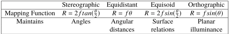
bootable USB. Figure 5.1 below, shows the operating system up and running with 4

(27)

Figure 5.1: A screen capture of the working Ubuntu 14.04 environment

5.2 ROS

As discussed above, the Indigo release of ROS was selected because of the

sup-ported packages related to USB cameras. Also a quick Google query illustrated

that there was much more thorough documentation related to bugs and common

problems for Indigo as opposed to Kinetic Kame. With that in mind, I followed the

installation steps outlined on the ROS website (http://wiki.ros.org/indigo/

Installation/Ubuntu_{). I opted for the full desktop install, as this machine was}

entirely devoted towards running Linux, ROS, and OpenCV for this project. The

first additional stack that had to be installed was the camera_umd stack. Inside of

this stack were three libraries: camera_umd, jpeg_streamer, and uvc_camera. It

was the last library, uvc_camera that I was most interested in because this library

had the launch files for USB cameras. While this library made it possible to run

the USB camera as a node in the operating system, it did not allow for the user

to see the image. To display the image, the aptly named image_view library was

utilized. The simplest way of using that library just subscribed to the user identified

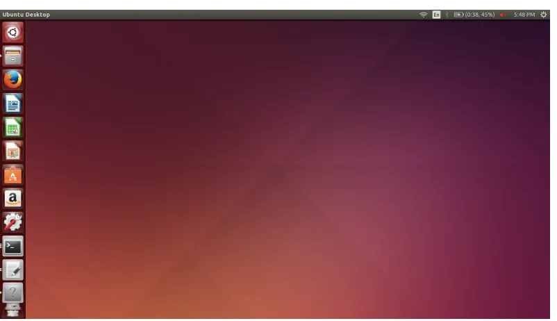
topic, and streamed the images from the camera to the user in a window. The figure

below shows the USB camera successfully running on ROS and being displayed via

(28)

Figure 5.2: A screen capture showing the camera successfully running and display-ing as a ROS node. The terminal on the left is runndisplay-ing the camera node. The upper right terminal is displaying the image using image_view and finally the bottom right terminal is running the main roscore.

5.3 OpenCV

OpenCV is a library of programming functions that are geared for real-time computer

vision. It was originally developed by Intel and is now managed by Itseez. It is

an open source software that can be downloaded from Github and easily installed.

For this project I tried to download one of the most recent releases, OpenCV 3.1.

Unfortunately, after installing it and trying to use it in conjunction with cv_bridge,

the program kept segfaulting. After trying to debug this issue with Dr. Kun Li,

we finally discovered a StackOverflow question that declared there was still not fix

to solve the compatibility issues between OpenCV 3 and cv_bridge. As a result, I

had to uninstall this release and download OpenCV 2.4.13 instead. The files were

finally installed and the OpenCV environment was built.

5.4 cv_bridge

To connect ROS to OpenCV I used a library built into ROS called cv_bridge.

There was an online tutorial on the ROS wiki that demonstrated how to convert

an image from the ROS encodings to the OpenCV encodings and then display it

after transforming it into a numpy matrix. The figure below illustrates a successful

(29)

the upper left corner.

A simple break down of how cv_bridge works is that is subscribes to a specified

topic. It also establishes a publisher that is normally called image_converter. So

the packages are received from the topic that is predecided and then the cv_bridge

transports it into OpenCV format. A display of this working is displayed below.

Figure 5.3: The display window on the left is the output from the image in OpenCV. The display window on the right is the direct stream from the fisheye camera itself. The reason for the discrepancy between the images is the different encodings the image takes on in the two systems.

5.5 External Hardware

In order to get the whole system to work as a single unit in space, the camera had

to be successfully mounted on a stand. This stand was designed in SolidWorks and

fabricated using the Dimension 3D Printer in the shop. The CAD for the stand is

displayed below. The board for the camera already had four pre-drilled holes in

the corner. The design capitalized on those holes as mounting points and locked in

the camera so that the lens faced directly up. The first iteration includes no way of

(30)

Figure 5.4: A screenshot of the fisheye camera housing that I created in SolidWorks. It will be fabricated using a 3D printer.

The housing was designed so that the pillars in the 3D print would interact with the

pre-drilled holes in the chip as a slip fit. After printing the housing, it became clear

that the tolerances were not as fine as they appeared to be in the CAD. As a result,

the fit transitioned from a slip fit to a press fit and the caps were no longer necessary.

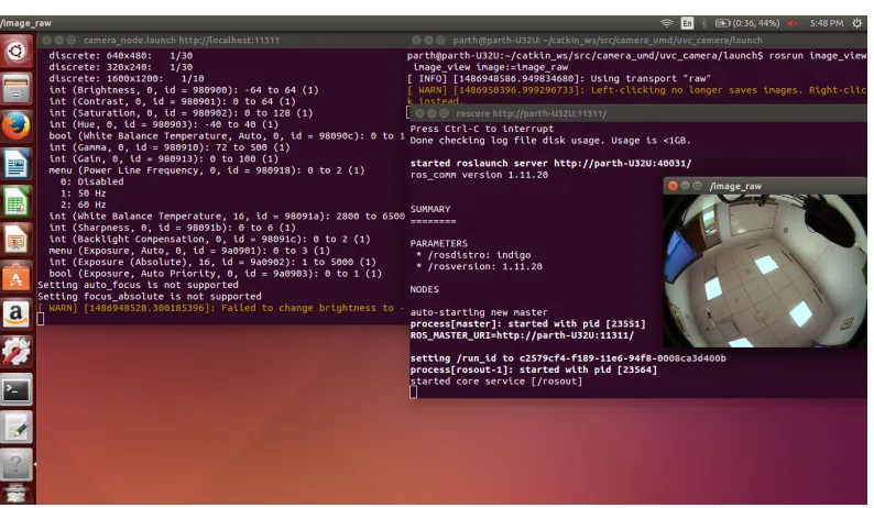
The installed version of the first iteration is displayed in Figure 5.5.

Figure 5.5: The fisheye camera successfully installed into the 3D printed housing.

Moving the project onto a quadcopter will be a very different task. Instead of

having a display and running the tasks through the host laptop, a small computer,

(31)

with the commands necessary to start the camera as a node and run the programs

(32)

C h a p t e r 6

IMAGE PROCESSING TO FIND AND TRACK THE SUN

6.1 Camera Parameters

Blooming is the phenomena where light streaks out of a light source saturating other

pixels. This is often seen in cameras when trying to capture very bright objects such

as the sun. With the fisheye camera that is being used, there are few variables that

can be manipulated. These different camera properties need to be best manipulated

in order to reduce the blooming effect of the Sun. The three variables that can be

varied are: white balance temperature, gain, and gamma of the image. Below I

present a side by side comparison of how each of these variables effects a LED light

source and the Sun.

First we need to present the control. In the figures below the LED light and the Sun

is captured with all three variables set to their minimum, which is the default. In the

control picture of the Sun, the blooming effect is clearly visible. As for the image of

the LED light, it is important to focus on how the areas surrounding the LED light

change. It is also important to note the presence of the halo from the glare of the

Sun.

Figure 6.1: The control image of the two light sources with the camera parameters set to their defaults.

Next we increase the white balance temperature to its maximum of 6500 Kelvin.

In photography the white balance temperature is used to denote the approximate

(33)

temperature should be set close to 5800 Kelvin. The images below display the

difference produced when the white balance temperature is set to its maximum. The

most obvious result is that the camera adds warm tones to the raw image, specifically

notice how the walls become yellower.

Figure 6.2: Outdoor and indoor images with the white balance temperature set to its maximum value of 6500 Kelvin. The camera adds warmer tones to the raw image.

The second variable that was increased to its maximum value of 6 was the gain. The

gain is used to boost the brightness of an image in low light conditions. However,

the gain cannot be used to reduce the brightness of an image, as is required when

shooting the Sun. The result of changing the gain from 0 to 6 is not very noticeable

as the two environments that we have captured are not poorly lit.

Figure 6.3: Increasing the gain value did not have much of an effect on the image. The gain effect only effects images that are taken in dark environments.

The final variable manipulated was the gamma value. Gamma defines the

(34)

this value ranges from 72 to 500. Normally this value is set at its minimum of 72.

By increasing this value to 500, the image should transform to a much brighter one.

This is clearly what is observed in the set of images below. The blooming effect

is definitely less noticeable with this change of gamma. However, it is not clear

whether increasing the gamma and making the image very bright will be worth the

reduction of the blooming effect. As a result, the gamma value will be set to its

minimum value of 72 unless stated otherwise.

Figure 6.4: Increasing the gamma value may have actually reduced the blooming effect but it came at the cost of the entire image becoming a lot brighter, thus making it more difficult to differentiate objects.

The final set of parameters that will be used with the camera include: white balance

temperature of 6500 Kelvin, gain of 0, and a gamma of 72. The image format

will be JPEG. The size of the image will be determined later when optimizing the

performance of the function against some error bound.

6.2 Encoding

The next experiment that will have to be performed before beginning the image

analysis is the encoding for the image in OpenCV. There are many different formats

the image can be reformatted to in OpenCV. It originally is transported to OpenCV

(35)

Figure 6.5: The original image published by the camera node. It is transported to OpenCV and its encoding at that point is RGB8.

It is clear that there exist a plethora of different encodings for images that are

compatible with OpenCV. Just to name a few, some of the possible encodings

include: GRAY (black and white), HSV (hue, saturation, and value), YUV (luma

and chrominance), and Bayer (half the pixels are filtered green). Initially it was

thought that transforming the RGB image to GRAY, as displayed below, would be

the dominant strategy because then it would be easy to isolate the white objects, the

sun, in the image.

(36)

However, after seeking advice from users familiar with image encodings another

encoding emerged as a possibility, HSV. HSV appeared to be another candidate

because it separated the image into three different matrices: hue, saturation, and

value. The object that we are concerned with is going to normally be the brightest

object in the image. For this reason, this value matrix is important because it

quantifies the magnitude of the brightness of that specific pixel in the image. The

hue matrix is displayed below in Figure 6.7. In reality, we will discard the hue and

saturation matrices and only focus on the value one.

Figure 6.7: Again using the cvtColor function in OpenCV the original RGB image is transfored to the HSV space. This figure displays the H (hue) matrix of this colorspace.

6.3 Thresholding

Once the value matrix of the image has been attained it needs to be thresholded.

This procedure will impose a mask on the value matrix. All values that are below

the predefined threshold will be set to 0. The resulting matrix, as displayed in

Figure 6.8, only reveals the brightest features. All the scales in the HSV encoding

range from 0 to 255. Originally the image was thresholded to accept the entire hue

spectrum, the entire saturation spectrum, but only the upper end, values above 225,

(37)

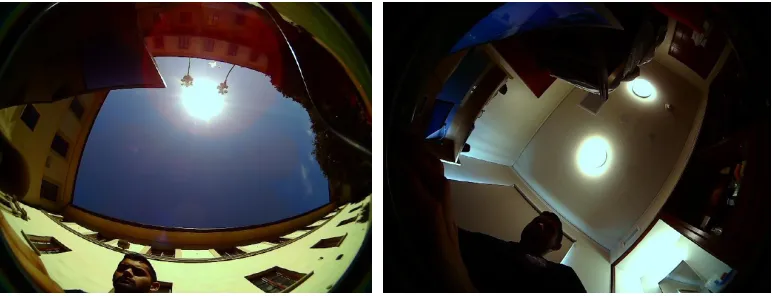
Figure 6.8: The masked image after it has been successfully thresholded. The white spaces are the only parts of the image that had value score greater than 225. The three objects on the left are lights in the room, and the large object on the right is the sky that is being illuminated by the sun.

Of course the thresholding bounds had to be iterated a few times before finally

arriving to the desired limit for the sun. Originally the threshold was tested on LED

lights inside of Gates-Thomas and the 225 value was sufficient. Unfortunately, when

testing the threshold function outside on a cloudy day, a limit of only 225 picked up

a lot of extraneous white objects such as clouds and white walls that reflect the sun

light. To reduce the number of extraneous objects that remain after the thresholding

the bound was increased to only accept value readings that were between 253 and

255.

6.4 Finding and Tracking

Originally the strategy to find the Sun was to sweep the image with a square

approximately the size of the Sun and determine what region had the highest value

score. This approach however has a runtime of O(n2) and there exist more efficient

methods to find objects in an image. After thresholding, our matrix is essentially a

binary matrix. There exist a set of functions already built into OpenCV that can help

us identify the groups of 1’s in the matrix. First we run the function findContours

which identifies all the groups of 1’s in the matrix by constructing convex hulls

around them. Then we create a circle that can enclose the convex hull using the

minEnclosingCircle function. This returns the center and radius of the enclosing

(38)

all the different contours we have found.

Now that we have all the different contours we need to identify which one is the

sun. Normally the Sun tends to be the largest contour in the image when we have

thresholded the image so strictly. For this reason we determine the index of the

contour with the largest radius and that is determined to be the Sun. Using the

OpenCV circle function, we can overlay a circle on the original image to denote the

contour with the Sun. The results of the first attempt to run this script is displayed

in Figure 6.9.

Figure 6.9: The result of the Sun finding script. The contour seems to have included a part of the cloud as well, and as a result the radius of the enclosing circle is larger than desired.

In Figure 6.9, the Sun is clearly partially obstructed by the roof. The threshold also

does not appropriately eliminate the entirety of the cloud that is near the Sun. As a

result the contour denoting the Sun is larger than it needs to be and includes a part

of the cloud. To fix this the threshold bounds need to be adjusted. It might also be

necessary to introduce a bias factor that bounds selected contour sizes above and

below. As of now we only have below in order to remove contours that appear as

a result of random white noise. By bounding the contour size above, we will bias

the script to only select contours that are similar to the size of the Sun. Further

data needs to be gathered to tune the bounds as to account for the size discrepancies

based on the distortion of the image.

Achieving the most rudimentary requirements for tracking is relatively easy. The

(39)

are running is set to find the Sun on every tenth image. We are also saving the

image after the Sun has been idenitified in a folder on the Desktop. The location of

the contour, the center of the circle, is written to a separate text file every time an

image is saved. This process blindly meets the requirement for tracking the Sun in

sequential images. However there are definitely more intuitive methods that can be

implemented to make the process more efficient.

6.5 Gaussian Blurring and Sobel Kernels

The next step is to see if some clever image processing tricks can be applied to get

around the bloom phenomena. The first is to see if it was normally distributed. This

does not appear to be the case because in consecutive images the phenomena tends

to appear in the same place. As a result it is not feasible to gather a large number

of images at once and then average the phenomena over the samples collected to

remove its impact. The other image processing trick that confirms that it is not

normally distributed is Gaussian blurring. This procedure takes a square matrix and

sweeps it over the image while reassigning the center pixel the average value of the

pixels in the matrix. This will ideally remove any streaky or randomly distributed

features in the image. Figure 6.10 illustrates the result of Gaussian blurring. It

diminishes some of the isolated bloom regions but also strengthens some of the

highly concentrated bloom regions. By strengthening these areas it does not remove

the shift in the centroid estimation, which is the root cause of error in heading

estimates.

(40)

The other image processing technique that can be implemented is an edge detector,

the Sobel kernel. The idea here is that maybe if the edge is better isolated and

apparent the contour fit might be tighter. The Sobel kernel takes the gradient in the

x and y direction before combining them to output the edge. The result of one pass

of the Sobel kernel is displayed in Figure 6.11. Unfortunately, the regions of bloom

do not falter and are present after the kernel has passed over. As a result, the contour

still finds the same expected fit and the error in the heading estimate persists.

Figure 6.11: The image shows the result of the edge detector, Sobel kernel. The bumpy outline of the Sun is due to the bloom phenomena. The roughness causes the centroid to be off, thus influencing the heading estimates.

Neither of these techniques seem as if they alone can impact the original finding

and tracking algorithm to nullify the presence of the bloom effect.

6.6 Erosion and SimpleBlobDetection

After discussing these issues with content experts, the persistence appears to be

dependent on the choice of preprocessing and estimation functions. Once the image

has been converted into the appropriate encoding and masked, there appear to

be some white streaks that occasionally influence the results of the findContour

function. A function that is strong in removing these patchy and streaky phenomena

is erosion. It takes a kernel similar to the one used in GaussianBlur, but instead

turns the center pixel to 0 if all its neighbors are 0 as well. A couple iterations of

this function leads to the removal of any streaky phenomena present around the Sun

(41)

The erosion function also helps remove the bloom effect, ever so slightly. Given an

ellipse, the erosion function will chip away at some of the awkward perimeter pixels

equally. But with the bloom effect present, because it increases the perimeter in that

region, it results in a slightly higher expected erosion in that region in comparison

to the rest of the perimeter of the Sun.

Once this modification has been applied to the image, only a circular or slightly

elliptical object should be left in the image. The findContour function would

identify this contour and then return the minimum bounding circle for the contour.

While this is a reasonable approach, even the slightest remains of the bloom effect

could cause significant changes in the heading estimate. The simpleBlobDetect

function however finds a blob and then returns a circle that best fits inside the blob.

The difference between the two functions is displayed in Figure 6.12 and in turn will

hopefully reduce the effects of the bloom effect.

Figure 6.12: The blue circle indicates "the Sun" as found by the findContour function. The red circle is the improvement after implementing a series of preprocessing functions along with simpleBlobDetect.

6.7 No Rectification or PSF

Calibrating the camera is important because it allows us to remove any distortions

and rectify the original image. This process can make it easier to determine where

the Sun actually is in order to calculate the error of the state estimation system. ROS

has a built in node, camera_calibration, that already has the necessary files to create

the appropriate calibration file. It requires the user to first print out a standard pattern

(42)

The .yaml file that will be created will contain the camera matrix, distortion vector,

and rectification and projection matrices. These matrices play a critical role in

rectifying the image before running the scripts to find and track the Sun.

In our case however, we do not appear to need to rectify the image. The

simple-BlobDetect should be able to outperform the traditional sweep we had originally

discussed. If the sweep of a constant size window was implemented, then the

recti-fication will be crucial. As a result, the matrices for the rectirecti-fication for the fisheye

camera have been stored, but will not be used unless the algorithm reverts back to

sweeping a constant size window across the image in search for the Sun.

The PSF also does not play a large role in this image processing portion because

we have already determined that the bloom effect is not normally distributed. As a

result, if we are to apply the deconvolution to remove the PSF, the Wiener filter, it will

not isolate and remove the bloom effect. As a result we disregard this phenomena

for now and focus on minimizing the impact of the bloom effect.

6.8 Further Improvements

A simple improvement that can be made to the tracking algorithm involves storing

the center location of the Sun in the prior image. This would require modifying the

desired data structure, to take the form of a modified linked list. The script can then

be changed to focus on blobs that are located near the prior center. This is all under

the assumption that there are no rapid maneuver performed with the robot. This is

reasonable because its path should be relatively predictable and this restriction can

be imposed on the planning algorithm. The only time there could be a quick change

in pose could be when the robot decides to make an aggressive maneuver and return

back to its home location. At this time the robot or helicopter will rotate quickly to

(43)

C h a p t e r 7

ESTIMATING HEADING

7.1 True Position

To acquire the true position data of the Sun we had to find an online calculator

published by a reputable source. The National Renewable Energy Laboratory has

two such calculators. Their first one is called SOLPOS and has valid data between

1950 to 2050 within a hundredth of a degree. Their other calculator has valid data

between -2000 and 6000 within a couple hundred thousandth of a degree. The

SOLPOS calculator exported the desired data between a certain time period as a zip

file very conveniently, so that is the one we used.

The user had to input the latitude, longitude, and time zone of their location along

with the desired output values. During this first iteration only the azimuth and zenith

angles of the Sun were output assuming the user was in Pasadena, California. We

asked the calculator to output data for ideal dates of the mission. The mission is

scheduled for 2020 and these types of missions normally have a lifespan of under

a couple years. Just to be conservative we asked the calculator for a six year time

period between 1/1/2020 and 1/1/2026. Unfortunately, the calculator only outputs

less than a million data points in one go. So the frequency of the data had to be

decreased to once every ten minutes. The text file containing the data for this six

year period had a size of 3.43 megabytes.

The data however included the position of the sun before sunrise and after sunset.

A script can be written to remove all these useless readings to shrink the size of the

file. Further investigation also needs to be done on whether the trajectory of the

sun is constant and can be extrapolated from two data points. Because our flights

will normally be less than ten minutes, we will have to rely on just two data points

or increase the frequency of the data we have stored from the SOLPOS calculator.

Ideally, we can just take the two nearest data points and extrapolate based on the time

on the clock to get where the Sun is. This would definitely save us some memory

(44)

7.2 Fixed Position, Heading Estimate Test

A couple different iterations of experiments were performed to test this algorithm.

The first one focused on reducing all potential moving parts and determining the

performance and accuracy of the algorithm. In this experiment the camera was

placed on a table on the roof of Gates Thomas and the algorithm output the azimuth

and zenith angles of the Sun. We did not have to worry about any motion of what

the camera was mounted to because in this experiment it was fixed to a table on the

roof.

Please note that from here on forward both the zenith and azimuth estimates will

be provided. When estimating the heading, we will only need the azimuth reading.

Both are provided as to further understand the impact between the variables altered.

There are a couple of parameters that should be noted before we dive into the results

of this experiment. The resolution of the images passed from the camera to the

algorithm was 640 by 480. The experiment was started at 10:30 am and ran till 6:30

pm. The table was placed on the gravel that was on the roof of Gates Thomas. This

resulted in the surface of the table being slightly tilted. Using a cheap level, the table

was tilted by approximately 1°. The first ten azimuth readings were also averaged and

compared against the first ten expected azimuth readings. The difference between

these values ended up being the rotation matrix applied to the rest of the data. The

algorithm that was implemented was also limited to the advancements made while

the findContour function was still in the code. The simpleBlobDetect function had

yet to be implemented.

The azimuth and zenith approximations were off by an average of 2.4° and 5.6°

respectively. Unfortunately, these results result in error bounds that are larger than

what we targeted. Looking back on intermediate images saved along the way it is

clear why the error is so large. Figure 7.1 shows the algorithm working as expected.

It finds the Sun in the image and only encloses the Sun while discarding parts of the

blooming effect that surround the Sun. Figure 7.2 however shows the opposite. Here

the algorithm drastically failed at excluding the bloom phenomena from the Sun. As

a result. the zenith approximation was off by 7°. The graphs off the approximations

(45)

Figure 7.1: The algorithm successfully identifies the Sun while excluding any of the surrounding bloom phenomena. The resulting estimates are within 2° and 3° respectively.

(46)

Figure 7.3: The two graphs showing the angle approximations against the true values. The zenith approximation started off wrong and strayed even further, while the azimuth approximation wavered around the true values.

7.3 Second Iteration

In the next iteration of the experiment, the resolution of the images was changed

from 640 by 480 to 2048 by 1560. The thresholding was also changed from 253

to 255 in an effort to reduce the impact of the bloom effect. As depicted in Figure

7.4, this resulted in the two approximations being off by an average of 3.6° and 6.6°

degrees in the azimuth and zenith values, respectively. This was worse than the

heading estimates produced when the image resolution was 640 by 480. Increasing

the threshold from 253 to 255 did not reduce the bloom effect. Those neighboring

pixels that are being saturated, tend to saturate to their maximum values, thus making

it difficult to distinguish them from the actual light source. The increased image

resolution allows for the bloom effect to be portrayed with a higher resolution. This

clarity of this phenomena biases the centroid more consistently, causing the estimates

to worsen with the change that was implemented. It is important to note that the

algorithm still used findContour instead of simpleBlobDetect in this iteration. The

(47)

Figure 7.4: The two graphs showing the angle approximations against the true values for the second iteration with higher resolution images and increased threshold values. Both the zenith and azimuth approximations worsened with these changes.

7.4 Third Iteration

In the third iteration of the fixed position, heading estimate test the image size

was reduced to 1024 by 768. The algorithm was also overhauled to include new

preprocessing steps such as erosion and gaussinBlur. The findContour function was

scrapped and was replaced with the simpleBlobDetect function. This experiment

was only two hours long but produced an error of 3.5° for the azimuth approximation.

This was definitely a step in the right direction. With a little bit more preprocessing,

it clear that the error can be brought down drastically using a script centered around

the simpleBlobDetect function.

(48)

Optimizing preprocessing techniques and fusing the sensor output with other sources

will improve the heading estimation accuracy.

7.5 Kalman Filter Model

In this section we will define the Kalman filter necessary to fuse the different heading

estimates into one.

The linear state space that describes the heading and angular velocity:

θk = " θ Û θ #

From dynamics we can conclude that:

θk =Fθk−₁

where:

F = "

1 ∆t

0 1 # G= " 1 0 # so that:

θk = Fθk−₁+wk

where:

wk ≈ N(0,Q)

Q =GGTσ2 a = " 1 0 0 0 # σ2 a

Suppose the measurement noise, vk is also normally distributed with mean 0 and

std devσz

zk = Hθ0_k+vk

(49)

R= h

σ2 z

i

We know the initial starting state of the TurtleBot with perfect precision so we

initialize it to:

ˆ

θ₀|₀ = "

0

0 #

P₀|₀ = "

0 0

0 0 #

Now that we have identified all of the elements, we must show how they are used.

First you must predict. We will show the two predictions, predict state estimate and

predict estimate covariance, respectively:

ˆ

θk|k−₁= Fkθˆk−₁|k−₁+Bkuk

Pk|k−₁ = FkPk−₁|k−₁F_kT +Qk

Please note that we have no Bu term because we have no known control inputs.

Instead we have a second sourceθ0and G applies it to the state vector.

The update steps then follow. First you find the innovation:

˜

yk = zk−Hkθkˆ |k−₁

Then calculate the innovation covariance:

sk = HkPk|k−₁HT_k +Rk

Now the optimal Kalman gain:

Kk = Pk|k−₁H_kTs−_k1

Finally update the state estimate and estimate covariance, respectively:

ˆ

θk|k =θˆk|k−₁+Kky˜k

Pk|k =(I−KkHk)Pk|k−₁

Thus we have successfully derived the Kalman filter necessary to fuse different

Heading Estimation via Sun Sensing for Autonomous Navigation

Navigation

Parth Shah

ACKNOWLEDGEMENTS

ABSTRACT

TABLE OF CONTENTS

LIST OF ILLUSTRATIONS

LIST OF TABLES

NOMENCLATURE

INTRODUCTION

BACKGROUND

OBJECTIVES

FISHEYE REVIEW AND ALGORITHM OVERVIEW

ENVIRONMENTS

IMAGE PROCESSING TO FIND AND TRACK THE SUN

ESTIMATING HEADING