Excel For Dummies Quick Reference.pdf

by John Walkenbach and Colin Banfield

Excel

2007

DUMmIES

Q U I C K R E F E R E N C E

by John Walkenbach and Colin Banfield

Excel

2007

DUMmIES

Q U I C K R E F E R E N C E

About the Authors

John Walkenbachis a leading authority on spreadsheet software and is principal of JWalk and Associates Inc., a small San Diego–based consulting firm that specializes in spreadsheet application development. He is the author of approximately three dozen spreadsheet books and has written hundreds of articles and reviews for a variety of publications, including PC World, InfoWorld, Windowsmagazine, and PC/Computing. John graduated from the University of Missouri and earned a master’s and a PhD from the University of Montana. Visit his Web site at www.j-walk.com. Colin Banfieldhas been working in the telecommunications field for more than twenty-five years and has been using spreadsheet programs for more than two decades. Colin’s largest Excel project to date is a comprehensive tool that is

designed for telephone central office equipment configuration, pricing, and manufac-turing and used by sales, engineering, and manufacmanufac-turing personnel. In between his telecom consulting duties, Colin works with organizations to extract information from corporate databases for business intelligence reporting in Excel. In his spare time, Colin writes and reviews books for Wiley and enjoys photography, astronomy, and expanding his musical repertoire. Colin holds a BSc (Honors) in Electrical Engineering from the University of the West Indies and has received extensive training in many advanced technologies.

Dedication

To Dorothy, my most loving and patient better half, and one of the nicest people on the planet. —C. B.

Author’s Acknowledgments

Thanks to the folks at Wiley who helped with the update of this book. In particular, my project editor, Susan Pink (Pinkie to me), did her usual wonderful editing and coordinating job and kept me on my toes. I’m indebted to Allen Wyatt, who provided a thorough technical review and made some very good suggestions for improve-ment. Finally, I’d like to thank David Gainer, Lead Program Manager for Excel at Microsoft, and his staff for clarifying some issues and for delivering this amazing update to a superb piece of software. —C. B.

Publisher’s Acknowledgments

We’re proud of this book; please send us your comments through our online registration form located at

www.dummies.com/register/.

Some of the people who helped bring this book to market include the following:

Acquisitions, Editorial, and Media Development

Project Editor: Susan Pink

(Previous Edition: Christine Berman)

Acquisitions Editor: Greg Croy Copy Editor: Susan Pink

(Previous Edition: John Edwards)

Technical Editor: Allen Wyatt Editorial Manager: Jodi Jensen

Media Development Manager:Laura VanWinkle Editorial Assistant: Amanda Foxworth

Composition Services

Project Coordinator: Heather Kolter, Ryan Steffen Layout and Graphics: Stephanie D. Jumper,

Barry Offringa, Lynsey Osborn, Heather Ryan Proofreaders:Dwight Ramsey, Evelyn Still,

Brian H. Walls Indexer: Techbooks

Publishing and Editorial for Technology Dummies

Richard Swadley,Vice President and Executive Group Publisher Andy Cummings,Vice President and Publisher

Mary Bednarek,Executive Acquisitions Director Mary C. Corder,Editorial Director

Publishing for Consumer Dummies

Diane Graves Steele,Vice President and Publisher Joyce Pepple,Acquisitions Director

Composition Services

Gerry Fahey,Vice President of Production Services Debbie Stailey,Director of Composition Services

Contents at a Glance

Part 1: Getting to Know Excel 2007 ...1

Part 2: Managing Workbooks ...21

Part 3: Working with Worksheets ...37

Part 4: Entering and Editing Worksheet Data ...49

Part 5: Using Formulas and Functions...77

Part 6: Creating and Using Names ...87

Part 7: Auditing Your Work ...97

Part 8: Formatting Your Data ...113

Part 9: Printing Your Work ...135

Part 10: Charting Your Data ...151

Part 11: Working with Tables ...169

Part 12: Goal Seeking and What-If Analysis ...185

Part 13: Analyzing Data with PivotTables...193

Glossary: Tech Talk...207

Index ...215

Part 13: Analyzing Data with PivotTables ...193

Anatomy of a PivotTable ...194

Changing the Summarization of a Value Field ...195

Creating a PivotTable Report ...195

Filtering a PivotTable Report...197

Filtering a PivotTable based on individual field items ...197

Filtering a PivotTable based on field data type ...198

Pre-filtering a PivotTable...199

Clearing PivotTable filters ...199

Formatting a PivotTable Report ...199

Applying a new style to a PivotTable ...199

Formatting based on data values...200

Changing the number format of a PivotTable field ...201

Grouping PivotTable Items ...202

Creating a date group ...202

Creating a number group ...203

Creating a text group ...204

Modifying a PivotTable Report ...204

Modifying a report layout ...204

Modifying a report structure ...205

Displaying and hiding subtotals and grand totals ...205

Expanding and collapsing field item levels ...206

Refreshing a PivotTable Report ...206

Glossary: Tech Talk...207

Index ...215

Table of Contents

xv

xvi

Getting to Know

Excel 2007

With Microsoft’s popular Excel 2007 spreadsheet program, you can enter, manip-ulate, and analyze data in ways that would be impossible, cumbersome, or error prone for you to do manually. This part gives you the basics you need to get up and running quickly in Excel.

In this part . . .

Familiarizing Yourself with the Excel 2007 Window Navigating with the Mouse and Keyboard

Introducing the Ribbon, Quick Access Toolbar, and Office Menu Formatting with Themes and Previewing Your Formatting Live

Part 1

Excel Basics

Excel documents are known as workbooks.A single workbook can store as many sheets as will fit into memory, and these sheets are stacked like the pages in a notebook. Sheets can be either worksheets(a normal spreadsheet-type sheet with rows and columns) or chart sheets(a special sheet that holds a single chart). Most of the time, you perform tasks in worksheets. In older versions of Excel (well, except for really old versions), each worksheet used a grid with 65,536 rows and 256 columns. Excel numbers rows starting with 1 and assigns letters to columns starting with A. After Excel exhausts the letters of the alphabet, column lettering continues with AA, AB, and so on. So column 1 is A, column 26 is Z, column 27 is AA, column 52 is AZ, column 53 is BA, and so on. Prior to Excel 2007, row numbers ranged from 1 to 65,536 and column labels ranged from A (column 1) to IV (column 256).

Excel 2007 increases the number of rows and columns in a single worksheet sig-nificantly. A worksheet now has 1,048,576 rows (no, that’s not a typo) and 16,384 columns (no, that’s not a typo either). Rows are numbered from 1 to 1048576 and columns are labeled from A to XFD.

The intersection of a row and a column is called a cell.A quick calculation using Excel tells me that this works out to 17,179,869,184 cells — more than enough for just about any use. Cells have addresses,which are based on their row and column. The upper-left cell in a worksheet is called A1, and the cell down at the bottom right is called XFD1048576. Cell K9 (also known as the dog cell) is the intersection of the eleventh column and the ninth row.

You might be wondering about the amount of system memory (known as random access memory, or RAM) you need to accommodate all those rows and columns. The actual memory you need depends on the amount of data you store in the workbook and the number of open workbooks. The good news is that Excel 2007 allows you to work with more memory than previous versions. Excel 2003, for example, will utilize up to only 1 GB (gigabyte) of memory, even if your system has more memory available. In Excel 2007, the memory available is limited by the max-imum amount of memory that your version of Windows (XP or Vista) can use.

Formulas

A cell in Excel can hold a number, some text, a formula, or nothing at all. You already know what numbers and text are, but you may be a bit fuzzy on the con-cept of a formula. A formulatells Excel to perform a calculation using informa-tion stored in other cells. For example, you can insert a formula that tells Excel to add the values in the first 10 cells in column A and to display the result in the cell that contains the formula.

2

Formulas can use normal arithmetic operators such as + (plus), — (minus), * (multiply), and / (divide). They can also use special built-in functions that let you do powerful things without much effort on your part. For example, Excel has functions that add a range of values, calculate square roots, compute loan payments, and even tell you the time of day. Part 5 covers how to use the various functions in Excel.

Active cell and ranges

In Excel, one of the cells in a worksheet is always the active cell. The active cell

is the one that’s selected, and it’s displayed with a thicker border than the others. Its contents appear in the formula bar.You can select a group, or range,

of cells by clicking and dragging the mouse pointer over them. You can then issue a command that does something to the active cell or to the range.

The selected range is usually a group of contiguous cells, but it doesn’t have to be. To select a noncontiguous group of cells, select the first cell or group of cells, hold down the Ctrl key while you drag the mouse, and select the next cell or group of cells.

Familiarizing Yourself with the Excel 2007 Window

Figure 1-1 shows a typical Excel 2007 window, with the important parts labeled. This terminology rears its ugly head throughout the book, so look at the figure carefully.

Moving, resizing, and closing windows

When Excel and workbook windows are in a restoredstate (between a maximized and minimized state, that is) you can use the resize handles to adjust the window size to your liking. Move the mouse pointer to the area of the resize handle until the pointer changes to a double-headed arrow, and then drag with the mouse.

You can move the window around the screen by dragging the title bars. See also

“Using the Mouse and Keyboard,” later in this part.

When the active workbook window is maximized, it shares a single Close button with the Excel window. After you click the shared Close button, Excel closes the active workbook.

Exiting Excel

Use any one of the following methods to close the Excel application:

Click the Close button on the Excel title bar if one or no workbook is open.

Click the Office button and then click the Exit Excel button.

Excel Basics — Familiarizing Yourself with the Excel 2007 Window

3

Double-click the Office button. See“Introducing the Office Menu,” later in this part.

Press the Alt key, then press F, and then press X.

Select all button

Control button

Name box Office button

Quick Access toolbar Excel title bar

Workbook title bar

Minimize Maximize/Restore

Close Help Split box

Workbook window Formula bar

Mouse pointer

Column header Active

cell pointer

Tab scrolling controls Sheet tabs

New sheet tab

Status bar Tab split

Normal view

Page layout view

Page break preview Scroll bar

Zoom controls

Split box

Window resize handles Row header

Figure 1-1

4

Navigating with the Mouse and Keyboard

The mouse is the primary tool that you use in Excel for executing commands, making selections, and navigating in the worksheet. Following are the mouse conventions that we use in this book:

Click:Click the left mouse button once.

Double-click:Click the left mouse button twice in quick succession. It may take you some time to get the hang of this action.

Right-click:Click the right mouse button once.

Drag:Hold down the left mouse button and move the mouse. Release the mouse button to complete the drag operation.

Hover:Place the mouse pointer over an element without clicking a mouse button.

Select:Place the mouse pointer over an element and click the left mouse button.

Mousing around

Every mouse action is associated with some element in the Excel window. An

elementcan be a slider, button, cell, chart object, and so on. You select or hover over the element using the mouse pointer.

Navigating through a worksheet with a mouse works just as you’d expect. Just click a cell, and it becomes the active cell. If the cell that you want to activate isn’t visible in the workbook window, you can use the scroll bars to scroll the window in any direction, as follows:

To scroll one cell, click one of the arrows on the scroll bar.

To scroll by a complete screen, click either side of the scroll bar’s slider button (the large center button).

To scroll faster, drag the slider.

To scroll a long distance vertically, press and hold the Shift key while drag-ging the slider button.

Note that only the active workbook window displays scroll bars. If you activate a different window, its scroll bars appear.

After you right-click a cell, a range of cells, or another object in the worksheet area, Excel displays a contextualmenu, so-called because the menu includes commands specific to working with the cell, range, or object.

Familiarizing Yourself with the Excel 2007 Window — Navigating with the Mouse and Keyboard

5

For your convenience, Excel 2007 adds a mini-toolbar above the contextual menu with useful commands drawn from the Ribbon, as shown in Figure 1-2. See also“Introducing the Ribbon,” later in this part.

Using the keyboard

Most users will be comfortable using the mouse to do all their work in Excel. For users who prefer to use the keyboard exclusively when working in Windows applications or for users who prefer to split the use of the mouse and keyboard among various tasks, Excel provides the following solutions.

Keyboard shortcuts

Keyboard navigation

KeyTips

The first two functions are described next. For more on the last function, KeyTips, see“Tipping off your keyboard,” later in this part.

You can access commands in Excel using keyboard shortcuts,which are individ-ual keystrokes or a combination of keys pressed simultaneously. To access the Print command using a shortcut, for example, you press and hold down the Ctrl key and press the P key, represented in this book as Ctrl+P. The following table lists some common keyboard shortcuts in Excel.

Shortcut

Action

Ctrl+A Select all

Ctrl+B Apply or remove bold formatting Ctrl+C Copy selection

Figure 1-2

6

Shortcut

Action

Ctrl+F Find

Ctrl+G or F5 Go To

Ctrl+H Replace

Ctrl+I Apply or remove italic formatting

Ctrl+O or Ctrl+F12 Open a document

Ctrl+P Print

Ctrl+S or Shift+F12 Save

Ctrl+U Apply or remove underlining

Ctrl+V Paste

Ctrl+W or Ctrl+F4 Close the active workbook

Crtl+X Cut

Ctrl+Y or F4 Repeat the last action

Ctrl+Z Undo the last action F1 Display the help viewer

Ctrl+F1 Hide or display the Ribbon commands F2 Enable editing within the active cell

With more than 17 billion cells in a worksheet, you need ways to move to spe-cific cells. Fortunately, Excel provides you with many techniques to move around a worksheet. As always, you can use either your mouse or the keyboard on your navigational journeys. The following table lists the keystrokes that enable you to move through a worksheet.

Keys

Action

Up arrow Moves the active cell one row up Down arrow Moves the active cell one row down

Left arrow Moves the active cell one column to the left Right arrow Moves the active cell one column to the right

PgUp Moves the active cell one screen up PgDn Moves the active cell one screen down

Alt+PgDn Moves the active cell one screen right Alt+PgUp Moves the active cell one screen left

Home Moves the active cell to the first column of the row that the active cell is currently in

Navigating with the Mouse and Keyboard

7

cont.

Keys

Action

Ctrl+Home Moves the active cell to the beginning of worksheet (A1) F5 Displays the Go To dialog box

Ctrl+Backspace Scrolls the screen to display the active cell

Up arrow* Scrolls the screen one row up (active cell doesn’t change)

Down arrow* Scrolls the screen one row down (active cell doesn’t change) Left arrow* Scrolls the screen one column left (active cell doesn’t change)

Right arrow* Scrolls the screen one column right (active cell doesn’t change)

* With Scroll Lock on

Introducing the Ribbon

Excel 2007 comes with a new user interface that replaces the standard menus and toolbars found at the top of the window in previous versions of Excel. The new interface is called the Ribbonand consists of a series of tabs, each contain-ing a variety of commands grouped accordcontain-ing to function (see Figure 1-3). Virtually all the features in Excel 2007 are available through the commands in the Ribbon tabs. This arrangement allows you to discover features in the pro-gram far more easily than if you had to drill down several layers into menus.

Dissecting the parts of the Ribbon

The commands in the Ribbon are accessed through a variety of controls. Here’s a list of the various types of controls and other parts that make up the Ribbon:

Button:This is the most common type of control. Most buttons in the Ribbon (except the formatting ones) have descriptive text associated with them, so you don’t need to be a Mensa expert to figure out what a button represents. The most frequently used commands in each Ribbon tab have larger buttons.

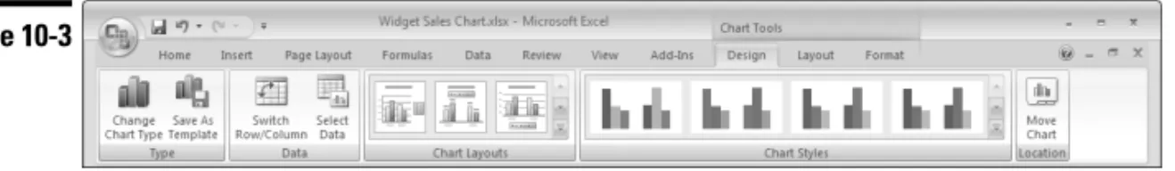
Contextual tab header Home tab

Split button Dialog launcher Contextual tabs

Figure 1-3

8

Help button:On the far right of the Ribbon is the help button (the question mark). Click this button for general Excel help.

Menu, rich: Rich menus are new in Excel 2007. Each menu choice has an illustrative graphic, the command name, and in some cases a short description of what the command does.

Don’t confuse rich menus with drop-down galleries, although they look similar. Menus contain related commands. Galleries allow you to choose from among a set of formats or layouts.

Menu, standard: Most users are already familiar with this form of menu — a drop-down list of choices with command names (such as Paste or Insert Cells). Some command names have small associated icons. If you click a command name that ends with an ellipsis (...), Excel displays a dialog box that presents further choices.

Spinner:A control with two arrows (one pointing up, the other pointing down) used with an input box to specify a number (height or width, for example.) Clicking an arrow increases or decreases the number in the input box. You can also enter a number in the box directly. The spinner control allows you to use only valid numbers.

Tab, contextual:Contextual tabs give the Ribbon the power to expose all features in Excel. One or more contextual tabs appear after you insert or select an object, such as a chart, shape, table, or picture. For example, after you insert a chart, three contextual tabs related to chart functionality appear on the Ribbon and a header labeled Chart Tools appears on the Excel title bar above the contextual tabs. Contextual tabs contain all the commands you need for working with the particular object. After you deselect an object, the contextual tabs (and the header) disappear.

The general rules that govern the display of contextual tabs follow:

• After you select an object (such as a chart, shape, or table), one or more contextual tabs for the object appear on the Ribbon. You must select a tab to display the associated commands.

• After you insert an object, Excel displays the commands for the first tab of the contextual tab set for that object.

• After you double-click an object, Excel displays the commands for the first tab of the contextual tab set for that object. Note that not all objects have this double-click capability.

• After you select, deselect, and then reselect the object without using any other commands in-between, Excel displays the commands for the first tab of the contextual tab set for that object.

10

Tab, standard:The Ribbon comes with a set of standard tabs, each organized according to the functions of the commands that it contains. For example, the Insert tab contains command groups to insert shapes, charts, tables, pictures, and so on. An exception is the Home tab, which is so-named because this is where you do most of your work in Excel.

If your mouse has a scroll wheel, you can navigate quickly among the Ribbon tabs by hovering the mouse pointer over the Ribbon area and scrolling the wheel back and forth.

Text box:A box in which you enter a number or text. In general, the Ribbon associates a text box with another control, such as a spinner or a drop-down box.

Sizing up the Ribbon

The layout of the Ribbon controls is not static. Depending on your screen resolu-tion, or the Excel window size, or both, the Ribbon provides one of four layout options for command groups. If sufficient space is available, the Ribbon presents a layout that labels commands, displays more commands individually, and elimi-nates extra clicks. As you resize the Ribbon downwards (by reducing the screen resolution or shrinking the size of the Excel window), the Ribbon rearranges the layout of some of the command groups by first resizing command buttons (larger buttons become smaller), then removing labels from commands, and finally reduc-ing the groups to sreduc-ingle large buttons (see Figure 1-4). To access the commands in a command group that the Ribbon resizes to a single button, you must first click the button to display a flyout menu and then select the command.

It is important to note that at each stage of downward resizing, no command groups or commands disappear entirely from the Ribbon. The multiple layout options for the command groups ensure that nothing is lost as space becomes more limited. If you reduce the size of the Excel window sufficiently, however, the Ribbon disappears altogether.

Figure 1-4

Introducing the Ribbon

11

Tipping off your keyboard

Excel provides a feature called KeyTips that allow you to access every command on the Ribbon using the keyboard, without having to memorize keystroke com-binations! So, what are KeyTips? KeyTips are little alphanumerical indicators containing a single letter, a combination of two letters, or a number, indicating what to type to activate the command under them, as shown in Figure 1-5.

Follow these steps to access a command in a Ribbon tab using a KeyTip:

1. Press the Alt key. The KeyTips appear over the Ribbon tabs (Ignore the KeyTips that appear in the other areas of the interface for this exercise.)

2. Press the key that represents the KeyTip for the Ribbon tab you want to access. For example, press N to select the Insert tab. Note that you do not

have to hold down the Alt key. If you need to select a different tab after you select the KeyTip for a tab, press the Esc key.

3. Press the key or key combination that represents the KeyTip for the com-mand you want to use.

If the command you select is a drop-down gallery or drop-down grid, you can use an arrow key or the Tab key to highlight your choice and then press the Enter key to select your choice.

Remember:KeyTips are associated with in-Ribbon galleries, so you have to press the key that represents the KeyTip for the gallery before you can choose an option in the gallery.

Remember:If the command you want to use requires a number key, you must use the number keys on the main keyboard. The KeyTip feature does not work with the numeric keypad.

Hiding the Ribbon commands

If you find that the Ribbon commands take up too much of your screen area, you can hide them using any of the following methods:

Press Ctrl+F1

Double-click any Ribbon tab

Figure 1-5

12

Right-click in the Ribbon area and choose Minimize the Ribbon from the contextual menu

Click the arrow to the right of the Quick Access toolbar and choose Minimize the Ribbon from the menu

If you click a tab after you hide the Ribbon commands, Excel displays the tab commands temporarily. The command display is hidden again after you select a command in the tab or click away from the Ribbon area. Similarly, you can use KeyTips to select a command when the command display is hidden.

To redisplay the commands permanently after you hide them, use the same methods described for hiding the commands.

Remember:Excel maintains the hidden condition of the Ribbon commands if you exit and subsequently re-launch Excel.

Introducing the Quick Access Toolbar

The Quick Access toolbar is an area of the new user interface that provides quick access to commands. The toolbar is designed to reduce the amount of navigation you have to do in the Ribbon to access the features that you use fre-quently. The Quick Access toolbar is on the left side of the screen, above the Ribbon and to the right of the Office button (see Figure 1-6).

The Quick Access toolbar is the only area of the new user interface that you can customize by adding commands to the three default commands (Save, Undo, and Redo).

Follow these steps to add a command to the toolbar:

1. Select the Ribbon tab that houses the command you want to add.

2. Right-click the command and choose Add to Quick Access Toolbar in the menu that appears.

To quickly add some common commands to the Quick Access toolbar, click the arrow to the right of the toolbar and choose a command from the menu.

You can add an entire command group to the Quick Access toolbar. Just right-click an area in the command group name (for example, Font) and choose Add to Quick Access Toolbar.

Figure 1-6

Introducing the Ribbon — Introducing the Quick Access Toolbar

13

Follow these steps to remove a command (including the default commands) from the toolbar:

1. Right-click the command you want to remove from the toolbar.

2. Choose Remove from Quick Access Toolbar in the menu that appears. If you think you’ll be adding a lot of commands to the Quick Access toolbar, it’s a good idea to move the toolbar from the title bar to a separate location below the Ribbon. Right-click anywhere on the toolbar and choose Place Quick Access Toolbar below the Ribbon in the menu that appears. You can regain screen area for working in the worksheet by double-clicking a Ribbon tab (or pressing Ctrl+F1) to hide the Ribbon controls temporarily.

You can access commands on the Quick Access toolbar using the keyboard. Press the Alt key and then a number key that represents the KeyTip for the command you want to access. See also“Tipping off your keyboard,” earlier in this part.

Introducing the Office Menu

Excel 2007 introduces a new menu for working with documents and accessing special Excel options. The menu is accessed by clicking the Office button (the large round button with the Office logo), located at the top-left corner of the Excel screen. See Figure 1-7.

Figure 1-7

14

The menu is divided into two sections. The left section contains a list of document-related commands. By default, the right section displays a list of recently used documents. Click a document name in the list to open the file. Click a pushpin to the right of a document name to keep the document on the list permanently. By default, Excel lists 17 documents, which get overridden with new documents unless you use the pushpin control. Some file commands on the left section include a built-in or attached arrow. If you hover the mouse pointer over a com-mand with an attached arrow, you will see a clear demarcation between the button and the arrow. Clicking a button with a built-in arrow or the arrow por-tion of a button with an attached arrow displays addipor-tional choices in the right section of the menu.

The Office menu also includes a button to access various Excel options and a button to exit Excel. We encourage you to visit the options from time to time, because you may find useful application, workbook, or worksheet options that you want to turn on or off. An option in the Advanced section of the Excel Options dialog box, for example, allows you to increase the number of docu-ments displayed in the Recent Docudocu-ments list to a maximum of 50.

Previewing Your Formatting Live

New in Excel 2007 is a Live Preview feature. When you hover over a formatting option with the mouse pointer, Excel lets you see the effect that the formatting option will have on your selection beforeyou commit to applying the option. Your selection might be a cell, range of cells, chart, table, shape, and more.

Suppose that you want to change the font of some text in a cell. In the Ribbon, a drop-down box called the font picker presents a list of available fonts. As you hover over each choice in the font picker, your cell updates to show you what the text would look like if you chose that font. Live Preview avoids the normal tedium of committing to an option, then undoing the option because the result is not what you wanted, and then committing to another option, only to realize that you don’t like the new result either, and so on.

You will find Live Preview options throughout Excel in places where formatting alternatives are available — most notably in galleries.

Formatting with Themes

In Excel 2007, you can now use a formatting concept known as a theme.A theme

consists of a combination of fonts, colors, and effects that provide a consistent look among your workbook’s elements, including cells, charts, tables, and PivotTables. You apply the theme’s fonts, colors, and effects through individual options or the style galleries of the various elements.

Introducing the Quick Access Toolbar — Formatting with Themes

15

Excel applies a default theme to all new workbooks along with a theme gallery so that you can change the default theme. After you select a new theme, all gal-leries and all the elements in your workbook formatted with theme styles change to match the new theme.

Following is a description of the three parts of a theme:

Theme font:A theme uses two complementary fonts — a header font and a body font. All elements using themed styles thus use the same font or fonts. Click the arrow on the drop-down box (called the font picker) in the Ribbon’s Home tab to see the fonts used in the theme currently applied to the workbook.

Theme color:A theme uses a matched set of twelve colors. Click the arrow on the Fill Color or Font Color tool in the Font group of the Home tab to see ten of the colors used in the theme currently applied to the workbook (see Figure 1-8).

The following are characteristics of theme colors:

• The top row in a color picker displays the base theme colors, and the next five rows display various tints and shades of the base colors. Below the theme colors are standard colors that do not change if the theme is changed. If you want to apply specific formatting that doesn’t change after you change the theme, use a standard color.

• The first four colors on the picker (from the left), are intended for text and background use. These colors are designed so that light text always shows well on a dark background, and vice versa.

• The next six colors are used for accents. Most of the theme-style gal-leries in Excel make extensive use of accent colors.

The two colors that are not exposed on the color pickers are used for hyperlinks (not discussed in this book).

Theme effect:Theme effects apply to graphic elements such as charts and shapes and include three levels of styles for outlines, fills, and special effects. Special effects include shadow, glow, bevel, and reflection.

Figure 1-8

16

You can change the theme in a workbook by clicking the Themes button in the Ribbon’s Page Layout tab and selecting a new theme from the gallery that appears.

Remember:The three Microsoft Office applications — Excel 2007, Word 2007, and PowerPoint 2007 — share the same themes. If you create reports that combine elements from each application, your reports will have a consistent look if you use a common theme.

Soliciting Help

With so many features and options available in Excel, it isn’t unusual to get stuck once in a while. Fortunately, Excel provides the following methods for get-ting help easily:

Enhanced ScreenTips:Standard ScreenTips (also called ToolTips) have been available in Excel for some time and provide textual context to commands. After you hover your mouse pointer over a command in earlier versions of Excel, Excel displays the action of the command using either a single word (such as Paste) or a brief phrase (such as Increase Font Size). A standard ScreenTip helps to decipher the meaning of a command button, for example, when the button has no associated text and the command meaning is unclear from the button icon.

Enhanced ScreenTips take the concept a step further by adding a short description explaining the purpose of the command (hence the prefix

Enhanced). Some Enhanced ScreenTips include an explanatory graphic when a text description is insufficient to explain the meaning of the com-mand. Enhanced ScreenTips are available for all commands on the Ribbon. In many cases, the ScreenTip explanation provides enough information, so you don’t have to seek additional help. By default, Excel 2007 uses

Enhanced ScreenTips for all commands.

Contextual help:If the Enhanced ScreenTip doesn’t offer enough for you to understand the use of a specific command, you can get more detailed help. After you hover the mouse pointer over the command, the Enhanced ScreenTip that pops up lets you know whether additional help for the com-mand is available by indicating that you can press F1 for more help.

If you are in a dialog box and need help for the dialog box options, press the help button (the question mark) to get contextual help.

General help:Click the help button (the question mark) on the right side of the Ribbon or press F1 when you are not in a specific context (for exam-ple, the mouse pointer is not hovering over a command in the Ribbon) to display a list of general help topics.

Formatting with Themes — Soliciting Help

17

When you use contextual help or general help, Excel displays the help viewer, shown in Figure 1-9. The viewer sports Internet browser-style controls. In fact, it was built using the same technology that Microsoft uses in its Internet Explorer browser application. Of course, the viewer is not a full-fledged browser because you can view only Excel help content.

Back Forward

Stop Refresh

Home Print Search box

Text size

TOC

Pin

Go (search)

Search scope Minimize

Maximize/Restore

Close

Status bar

Search result window

Connection status

Figure 1-9

18

The major features of the help viewer follow:

Search box:You can enter specific search text in this box. The viewer stores a list of your text searches for the current help session. Click the drop-down arrow on the side of the box to view and select an item from the list if you want to review a previous search result.

Search button:Click the Search button (or press Enter) to initiate a search after you enter the search text in the search box. Click the arrow next to the search button to define the search scope. By default, if your computer is connected to the Internet, Excel will display help content from an online source. If possible, you should use this source as your first choice because Microsoft updates the contents of online help regularly.

If you are offline when you initiate a search, Excel uses help content inter-nal to your system. You can force Excel to use interinter-nal help content always by clicking the arrow next to the Search button and choosing Offline Excel Help from the menu.

Whether online or offline, you can narrow you search scope further by selecting an appropriate option from the Search button menu.

Search result window:This window displays the results of your search request. If you use contextual help or enter text in the search box, the window displays help information specific to the context of the search. If you use general help, the window displays a list of general help topics in the form of titled links. Clicking a link displays a new set of links with more specific titles. Click the specific link title that best matches your search cri-terion to display detailed information on the topic.

Status bar:The left side of the status bar (located at the bottom of the help viewer) displays the current search scope. The right side of the status bar displays the connection status. You can click in the connection status area to switch quickly between viewing online and offline help content.

Maximize/Restore button: Click this button for a full-screen view of the help window. Click again to restore the window to its previous size.

Minimize button:Click this button to hide the help viewer window. Click the Help button on the Windows taskbar (normally located below the Excel window) to redisplay the viewer.

Close button:Click this button to close the help viewer.

Pin button:By default, Excel keeps the help viewer window on top when you are working in the application. Use the Pin button to control this behavior. If you “unpin” the viewer, Excel hides the window automatically if you click anywhere inside the Excel window.

Soliciting Help

19

TOC (Table of Contents) button:Click this button to display a Table of Contents pane on the left side of the help viewer. The pane displays the same list of topics that the main windows displays after you select general help or click the Home button. Clicking a main topic in the pane displays a list of subtopics, similar to the subtopics that the main windows displays after you click a general help topic link. The Table of Contents pane is con-venient if you want to view the details of multiple subtopics in succession.

Text size button:Click this button to select a size for the text in the search result window.

Print button:Click this button to print the help topic that the search result window displays.

Home button:After browsing multiple helps topics in the search result window, you might want to return to the list of main help topics to choose another general topic link. Click the Home button to return to the list of main help topics.

Refresh button:Click this button to refresh the help topic list after you connect or disconnect from the Internet while the help viewer is open.

Stop button:Click this button to cancel a search request if the help viewer is experiencing difficulties connecting to the online help source.

Back and Forward buttons:After browsing multiple helps topics in the search result window, you might want to navigate among results and various levels of detail. Click the Back or Forward button to perform your navigation.

If you want to resize the help viewer window, move the mouse pointer to any edge of the window until the pointer changes to a double-headed arrow, and then drag the mouse.

20

Managing Workbooks

Working with documents is critical to using any software. Microsoft Excel docu-ments are known as workbooks.This part covers the procedures that you need to know to manage workbook documents efficiently.

In this part . . .

Arranging Windows Automatically Comparing Two Workbooks Side by Side Creating an Empty Workbook

Creating Multiple Windows (Views) for a Workbook Opening and Saving Files

Protecting and Unprotecting a Workbook Working with Workbook Templates

Part 2

Activating a Workbook

A workbook is activewhen its window is maximized in the Excel window or after you select any part of the workbook when its window is not maximized. See also

“Familiarizing Yourself with the Excel 2007 Window,” in Part 1 and “Switching among Open Workbooks,” later in this part.

Arranging Windows Automatically

If you want all your open workbook windows visible on-screen, you can move and resize them manually — or you can have Excel do it automatically. Follow these steps to make all open workbooks visible on the Excel screen:

1. Click the View tab in the Ribbon.

2. Click the Arrange All button. Excel displays the Arrange Windows dialog box.

3. Choose from the Tiled, Horizontal, Vertical, or Cascade options.

4. Click OK.

You can save the layout of your open workbooks for future use. See“Using a Workspace File,” later in this part.

See also“Comparing Two Workbooks Side by Side,” later in this part.

Changing the Default File Location

When you’re opening a document in Excel, by default the Open dialog box points to the My Documents folder (Windows XP) or the Documents folder (Windows Vista) as the starting location to open documents. If you keep fre-quently used documents in a different folder, you may want the Open dialog box to point to this different folder to save some navigation steps. To change the default folder, follow these steps:

1. Click the Office button, and then click the Excel Options button. The Excel Options dialog box appears. The options are divided into sections, which appear in a list on the left side of the dialog box.

2. Click the Save section.

22

3. In the Default File Location text box, enter the path of the new default starting location to open documents. For example, if your new default document location is in a subfolder named Excel, which itself is in the My Documents or Documents folder, add \Excel to the default path. The new location in the text box should read C:\Users\Username\Documents\ Excel, where Usernameis the actual name of the user indicated in the text box.

4. Click OK.

Closing a Workbook

If you’re no longer working with a workbook , you may want to close the work-book so that you can work on other documents without distraction. Closing unneeded workbooks also frees memory and minimizes potential screen clutter.

To close the unneeded workbook or workbooks, follow these steps:

1. If multiple workbooks are open, ensure that the workbook you want to close is active as follows: Click the View tab on the Ribbon, click the Switch Windows button, and select the workbook from the list of names in the menu.

2. Use any of the following methods to close the workbook: • Click the Office button and then choose Close.

• Click the Close button on the far right of the Ribbon tab area (or on the workbook’s title bar if the workbook is not maximized).

• Double-click the Control button on the far left of the workbook’s title bar if the workbook is not maximized.

• Press Ctrl+F4.

• Press Ctrl+W.

If you’ve made any changes to your workbook since the last time you saved it, Excel asks whether you want to save the changes before closing the workbook.

Activating a Workbook — Closing a Workbook

23

Comparing Two Workbooks Side by Side

Sometimes you have two versions of a workbook, and you want to compare the dif-ferences in the data visually. Excel provides a convenient feature that allows you to compare two documents side by side. To use this feature, follow these steps:

1. Open the workbooks you want to compare.

2. Click the View tab on the Ribbon and then click the View Side by Side button. Excel arranges the windows of the two workbooks horizontally. If you have more than two workbooks open, Excel displays a dialog box from which you select the name of the workbook you want to compare with the active workbook.

3. Click a worksheet tab in each workbook to display the worksheet data you want to compare.

4. In the View tab, click the Synchronous Scrolling button to toggle synchro-nized scrolling on and off. After you enable synchrosynchro-nized scrolling, the rows and columns in the two worksheets being compared scroll simultaneously.

5. You can click the Reset Window Position button in the View tab to ensure that the two workbook windows are sized equally and aligned horizon-tally. You need to use the button only if you adjust either or both window sizes during the current session.

You can save the layout of the open workbooks you’re comparing for future use.

See“Using a Workspace File,” later in this part.

Creating an Empty Workbook

After you start Excel, it automatically creates a new (empty) workbook that it calls Book1. If you’re starting a new project from scratch, you can use this blank workbook.

You can create another blank workbook in the following ways:

Press Ctrl+N.

Click the Office button, choose New, select Blank Workbook, and click Create.

You can add a button to the Quick Access toolbar that allows you to create a blank workbook with a single mouse click. Click the arrow to the right of the Quick Access toolbar and choose New from the menu. Excel adds the New button to the toolbar. See also“Working with the Quick Access Toolbar,” in Part 1.

24

Creating Multiple Windows (Views) for a Workbook

Sometimes, you want to view two parts of a worksheet at once. Or you want to see more than one sheet in the same workbook at the same time. You can accomplish either of these actions by displaying your workbook in one or more additional windows.

To create a new view of the active workbook, click the View tab on the Ribbon and then click the New Window button. Excel displays a new window for the active workbook. To help you keep track of the windows, Excel appends a colon and a number to the workbook name in each window, as shown in Figure 2-1.

See also“Arranging Windows Automatically,” earlier in this part, and “Comparing Two Workbooks Side by Side,” earlier in this part.

Remember:A single workbook can have as many views (that is, separate win-dows) as you want.

Displaying multiple windows for a workbook also makes copying information from one worksheet to another easier. You can use Excel’s drag-and-drop proce-dures to copy a cell, a range, or a chart. See also“Copying Cells and Ranges,” in Part 4, and “Resizing, Moving, Copying, and Deleting an Embedded Chart,” in Part 10.

Opening Nonstandard Files

In addition to files in its native format, Excel 2007 can open files in non-Excel 2007 formats, including older Excel and text files. Excel 2007 can open files that weren’t saved in its native format by using filters to open the foreign file as a workbook document.

Figure 2-1

Comparing Two Workbooks Side by Side — Opening Nonstandard Files

25

To open a file in a non-Excel 2007 format, follow these steps:

1. Click the Office button and then choose Open. Excel displays the Open dialog box.

2. Windows XP: In the Files of Type drop-down list, select the file type. Windows Vista: Click the button located above the Open and Close button and choose a file type from the menu. By default, the button text reads All Excel Files (*.xl*;*.xlsx;*.xlsm) but the text changes if you select a differ-ent file type.

3. Windows XP: In the Look In drop-down list, navigate to the folder that con-tains the file.

Windows Vista: In the Folders window on the left side of the dialog box, navigate to the folder that contains the document. If the Folders window isn’t displayed, click Folders.

4. Select the file and click Open, or double-click the filename.

See also“Opening a Workbook,” immediately following this section.

Opening a Workbook

If you open a workbook in Excel, the entire document loads into memory, and any changes that you make occur only in the copy that’s in memory.

To open an existing workbook , follow these steps:

1. Click the Office button and then choose Open to display the Open dialog box. Alternatively, press Ctrl+O or Ctrl+F12 to display the Open dialog box.

2. Windows XP: In the Look In drop-down list, navigate to the folder that con-tains the document.

Windows Vista: In the Folders window on the left side of the dialog box, navigate to the folder that contains the document. If the Folders window isn’t displayed, click Folder (see Figure 2-2).

3. Select the workbook in the selected folder and click Open, or double-click the filename.

You can select more than one document in the Open dialog box. The trick is to press and hold Ctrl while you click each document. After you select all the docu-ments you want, click Open.

26

Remember:You can open a workbook you have worked with recently without navigating through the Open dialog box. On the right side of the Office menu, Excel provides a Recent Documents list. If the document that you want to open appears in this list, you can choose it directly from the menu.

Protecting and Unprotecting a Workbook

Excel provides several levels of protection for your sensitive work. Here are some ways you can protect your workbooks. You can protect

A workbook from being opened by unauthorized personnel

A workbook from being saved with the same filename

A workbook’s structure (control the manipulation of worksheets in a workbook)

A workbook’s windows (control the sizing and positioning of a workbook’s windows and any workbook views you create)

You should write down any passwords you use and store them in a safe location. If you forget or lose your passwords, you won’t be able to undo the areas you protected by any normal means.

Safeguarding your workbook from unauthorized users

Follow these steps to restrict unauthorized personnel from opening or modify-ing a workbook:

1. Open a workbook or select an already opened workbook you want to protect.

Figure 2-2

Opening a Workbook — Protecting and Unprotecting a Workbook

27

2. Click the Office button and choose Save As. Excel displays the Save As dialog box.

3. Click Tools and choose General Options from the menu. Excel displays the General Options dialog box.

4. In the Password to Open text box, enter a password that must be used before a user can open the workbook.

5. In the Password to Modify text box, enter a password that must be used before a user can save the workbook under the same filename. Passwords can be up to 15 characters and are case sensitive.

6. Click OK. Excel asks you to reenter the passwords for confirmation.

7. Reenter the passwords.

8. Windows XP: In the Save In drop-down, select the folder in which to save the workbook and then click Save.

Windows Vista: If the Folders window isn’t displayed, click Browse Folders, click Folders to display the Folders window, and then select the folder in which to save the document. Then click Save.

9. If you’re saving the workbook with the same name, respond when Excel displays a message asking you to confirm overwriting the file.

To remove passwords from the workbook, follow the previous steps, except delete the passwords in Step 4, Step 5, or both.

See also“Saving Files,” later in this part.

If you are using a workbook saved in an earlier version of Excel, Excel 2007 displays a message offering to convert the workbook to the Office XML file format (the default file format) before you save the workbook with passwords. You should choose to accept the suggestion only if you will not be sharing the workbook with users who have earlier versions of Excel. See also“Saving Files,” later in this part.

The General Options dialog box offers other safeguarding options. Select the Always Create a Backup check box if you want Excel to always save a backup copy of the existing workbook before you save the workbook. If you select the Read Only Recommended check box, when the workbook is opened, Excel dis-plays a message suggesting that the workbook be opened as read only. The user, however, can choose to ignore the suggestion.

Protecting and unprotecting a workbook structure or window

To protect a workbook structure or window properties from accidental or inten-tional alteration, follow these steps:

28

1. Click the Review tab on the Ribbon and then click the Protect Workbook button. Excel displays the Protect Workbook dialog box.

2. Select the appropriate check box(es), as follows:

• Structureprevents any of the following changes to a workbook sheet: adding, deleting, moving, renaming, hiding, or unhiding.

• Windowsprotects the workbook window from being moved or resized.

3. If you feel that you need a high level of protection, supply a password in the Password text box, and click OK. When Excel requests that you reenter the password for confirmation, do so.

4. Click OK.

To unprotect a workbook structure or window, click the Review tab on the Ribbon and then click the Unprotect Workbook button. If you did not supply a password when the workbook was protected, Excel unprotects the workbook automatically. Otherwise, Excel prompts you to enter a password.

Saving Files

When you save a workbook, Excel saves the copy in memory to your drive — overwriting the previous copy of the workbook. When you save a workbook for the first time, Excel displays its Save As dialog box.

Excel 2007 uses a new default format for saving workbook documents. This new format is based on the Extensible Markup Language (XML). Office 2007 applica-tions use an extension to XML called Office Open XML. Workbooks saved in Office Open XML maintain full fidelity with everything in your document, includ-ing (in the case of Excel) formulas, formattinclud-ing, charts, tables, and macros. XML and Office Open XML are text-based formats (versus the binary formats found in earlier versions of Office applications).

You don’t need to have a complete (or even partial) knowledge of XML or Office XML to work in Excel 2007. However, it is useful to know that Excel 2007, like ear-lier versions, saves files with a different file extension depending on the type of file you are saving. A list of the standard file types and the extension names they use are given in the following table. We also include the corresponding file exten-sions used in earlier verexten-sions of Excel.

Protecting and Unprotecting a Workbook — Saving Files

29

File Type

2007 Extension

Pre-2007 Extension

Excel macro-enabled workbook .xlsm .xls

Excel workbook template .xltx .xlt Excel macro-enabled workbook template .xltm .xlt

Excel binary workbook .xlsb .xls

Excel add-in .xlam .xla

Excel workspace .xlw .xlw

Excel user interface customization* .xlb .xlb

* In Excel 2007, you can customize the Quick Access toolbar as we discuss in Part 1. In earlier versions of Excel, you can customize an existing menu or toolbar or create a menu or toolbar. Excel saves these customizations automatically in an .xlb file, whose location depends on the operating system you’re using (Windows XP or Windows Vista).

Remember:Unlike earlier versions of Excel, the table indicates that Excel 2007 workbooks or templates containing macros(scripts written to enhance Excel in some manner) are stored in files that differ from files without macros. If you attempt to save a macro-based workbook or template in a format that doesn’t support macros (.xlsx or .xltx), Excel gives you the option to save the file with-out macros or to select a format that supports macros (.xlsm or .xltm).

Saving a workbook

Use any of the following methods to save the active workbook:

Click the Office button and then choose Save.

Click the Save button on the Quick Access toolbar.

Press Ctrl+S.

Press Shift+F12.

If the document you’re saving does not yet have a name, Excel prompts you for a name by opening its Save As dialog box. You can give the document a name and navigate to the folder where you want to store the file. See also“Saving a work-book under a different name,” in the next section.

Saving a workbook under a different name

Sometimes you may want to keep multiple versions of your work by saving each successive version under a different name.

To save a workbook with a different name, follow these steps:

30

1. Click the Office button and then choose Save As. Excel displays the Save As dialog box.

2. Windows XP: In the Save In drop-down list, select the folder in which to save the workbook.

Windows Vista: If the Folders window isn’t displayed, click Browse Folders, click Folders to display the Folders window, and then select the folder in which to save the workbook (see FIgure 2-3).

3. In the File Name text box, enter a new filename. (You don’t need to include a file extension.)

4. Click Save.

Excel creates a new copy of the workbook with a different name, but the original version of the workbook remains intact. (Note that the original workbook is no longer open.)

Saving a workbook in a different or earlier file format

To share a workbook with someone who uses an application that opens files in a format other than Excel 2007, be sure to save the workbook in a file format that the other application can read.

Excel can save workbook contents in many non-Excel file formats, such as, tab-or comma-delimited text, html, and standard xml.

To save a workbook in a different file format, follow these steps:

Figure 2-3

Saving Files

31

1. Click the Office button and then choose Save As.

2. In the Save As Type drop-down list, select the format in which you want to save the file. For example, to save in an earlier Excel file format, select Excel 97-2003 Workbook.

3. Click Save.

Excel separates a list of some Excel file formats from the complete list of file types to save you time in navigating the Save As dialog box. Click the arrow at the end of the Save As option in the Office menu to display the list of some common Excel file formats.

Remember:If you attempt to save a workbook with features not supported in the file format you’re saving to, Excel displays a warning message. If the format you’re saving to is an earlier version of Excel, Excel displays the Compatibility Checker dialog box, which shows you a list of features that will be lost.

Switching among Open Workbooks

If you have multiple workbooks open, the workbooks usually appear maximized on-screen so that you can view only one workbook at a time.

To switch the active display among workbooks, use one of the following methods:

Click the View tab on the Ribbon, click the Switch Windows button, and then select one of the workbook names in the menu that appears.

Press Ctrl+F6 or Ctrl+Tab to cycle the active display among the open workbooks.

Using a Workspace File

The term workspacerefers to the layout of all the open workbooks — their screen positions and window sizes.

You may have a project that uses two or more workbooks, and you may like to arrange the windows in a certain way to make them easy to access at a later time. Fortunately, Excel enables you to save your entire workspace to a file. After you open the workspace file, Excel sets up the workbooks exactly as they were when you saved your workspace.

32

Opening a workspace file

To open a workspace file, follow the steps outlined for “Opening Nonstandard Files,” earlier in this part, except in Step 2, select Workspaces (*.xlw) from the drop-down list (Windows XP) or menu (Windows Vista). Excel opens all the workbooks that you originally saved in the workspace.

See also“Saving a workspace file,” the next section.

Saving a workspace file

To save your workspace, follow these steps:

1. Click the View tab on the Ribbon and then click the Save Workspace button. Excel displays the Save Workspace dialog box.

2. Use the filename that Excel proposes (for example, resume.xlw or resume), or enter a different name in the File Name text box.

3. Windows XP: In the Save In drop-down box, navigate to where you want to save the workspace.

Windows Vista: If the Folders window isn’t displayed, click Browse Folders, click Folders to display the Folders window, and then select the folder in which to save the workspace.

4. Click Save.

A workspace file contains not the workbooks themselves but only the informa-tion that Excel needs to recreate the workspace. Excel saves the workbooks in standard workbook files. If you distribute a workspace file to a coworker, there-fore, make sure that you also include the workbook files that the workspace file refers to.

Working with Workbook Templates

A workbook templateis basically a workbook that contains one or more work-sheets set up with formatting and formulas and ready for you to enter data and get immediate results. A workbook template can use any of Excel’s features, such as charts, formulas, and macros. Excel includes templates that automate the common tasks of filling in invoices, expense statements, and purchase orders. You can also download several more templates from the Internet. You can also create your own templates from scratch or from an existing workbook.

Creating a workbook template

To save a workbook as a template, follow these steps:

Switching among Open Workbooks — Working with Workbook Templates

33

1. Click the Office button and then choose Save As.

2. In the Save As Type drop-down list, select Excel Template.

3. If you want to save the template in a subfolder of the Templates folder in Windows XP: Excel displays the Templates folder in the Save In drop-down list. Select the subfolder in the Save In drop-down list.

If you want to save the template in a subfolder of the Templates folder in Windows Vista: Click Browse Folders (if the Folders window isn’t dis-played) and click Folders to display the Folders window if necessary (the Templates folder is automatically selected after Step 2), and then select a subfolder.

To create a new folder in the Templates folder in which you can save the template, click the Create New Folder button in the Save As dialog box and give the new folder a name.

4. In the File Name box, enter a name for the template, and then click Save. Excel saves templates with an .xltx file extension. If your template con-tains macros, Excel gives you the option to save the template without macros or to save in a format that supports macros (.xltm). See also

“Saving Files,” earlier in this part.

You can also save a template in an earlier file format. In Step 2, select Excel 97-2003 Template from the Save As Type drop-down list box.

To prevent overwriting the template file when you create a new workbook from a template, always save your templates in the Templates folder or a subfolder within the Templates folder.

Creating a workbook from a template

If you create a new workbook that you based on a template, Excel creates a copy of the template in memory so that the original template, on disk, remains intact. The default workbook name is the template name with a number appended to it. For example, if you create a new workbook based on a template by the name of Report.xltx, the workbook default name is Report1.xlsx. The first time that you save a workbook that you create from a template, Excel displays the Save As dialog box so that you can give the file a new name.

To create a workbook from a template, follow these steps:

1. Click the Office button and then choose New. Excel displays the New Workbook dialog box, as shown in Figure 2-4.

2. Select a template category from the list on the left side of the dialog box. The choices are as follows:

34

• Blank and Recent:This is the default category. From here you can select Recently Used Templates. Select a template and click Create to open a copy of the template file.

• Installed Templates:This category displays a gallery of templates installed in your system. Select a template and click Create to open a copy of the selected template.

• My Templates:This category contains templates you previously saved in the Templates folder or in a subfolder in the Templates folder. Click My Templates to display the New dialog box. Templates you create in the Templates folder appear in the My Templates tab. If you saved Templates in one or more subfolders in the Templates folder, the folder names appear as tabs in the New dialog box. Select a template from a tab and click OK. Excel opens a copy of the template.

• New from Existing:This category allows you to use any workbook as a template or to use a template file that’s not in the Templates folder. Click New from Existing to display the New from Existing Workbook dialog box. Navigate to the folder containing the file you want to use as a template, select the file in the folder, and click Create New. Excel opens a copy of the file.

• Microsoft Office Online:If you are connected to the Internet, you can select from one of the online categories and Excel will display a list of available templates in the selected category. Choose a template, click Download, and Excel opens a copy of the template.

3. Save the workbook after you enter the appropriate data in the template copy. See also“Saving Workbooks” and “Creating a workbook template,” earlier in this part.

Figure 2-4

Working with Workbook Templates

35

Creating a default workbook template

You can create a default workbook template that defines the formatting or con-tent of the new (blank) workbooks that open after you start Excel. Excel bases every new (blank) workbook that you open on the default workbook template. The default workbook template that you create replaces Excel’s built-in default workbook template.

Follow these steps to create a default workbook template:

1. Create a new workbook. See“Creating an Empty Workbook,” earlier in this part.

2. Add or delete as many worksheets as you want to appear in the new work-book. See“Adding a New Worksheet” and “Deleting a Worksheet,” both in Part 3.

3. If you want, turn off the display of gridlines. See “Turning off Gridlines,” in Part 3.

4. Apply the desired formatting, sheet names, text, styles, and so on.

SeePart 8 if you need help applying different formatting options.

5. Select a new theme for the template if you don’t like Excel’s default choice. See“Formatting with Themes,” in Part 1.

6. Click the Office button, choose Save As, and select Excel Template from the Save As Type drop-down list.

7. Windows XP: In the Save In drop-down list, locate an xlstart folder. Excel can use more than one xlstart folder and will open all files located in these folders on startup. The xlstart folders normally reside in the following locations: C:\Documents and Settings\Username\Application Data\ Microsoft\Excel (where Usernameis your login username) and C:\ Program Files\Microsoft Office\Office 12 folders, respectively.

Windows Vista: If the Folders window isn’t displayed, click Browse Folders, click Folders to display the Folders window, and then locate the xlstart folder. Excel can use more than one xlstart folder and will open all files located in these folders on startup. The xlstart folders normally reside in: C:\Users\Username\AppData\Roaming\Microsoft\Excel (where Usernameis your login name) and C:\Program Files\Microsoft Office\Office 12 folders, respectively.

8. In the File Name text box, type book.xlt.

9. Click Save.

All new (blank) workbooks that you create are now replicas of the book.xlt work-book that you saved in Step 9.

You can always edit the book.xlt file or delete it if you no longer want to use it.

36

Working with

Worksheets

A workbook can consist of any number of worksheets.Each sheet has a tab that appears at the bottom of the workbook window. In this part, we discuss several useful things that you can do with worksheets.

In this part . . .

Adding and Deleting Worksheets Changing a Worksheet’s Name

Grouping and Ungrouping Worksheets Hiding and Unhiding a Worksheet Protecting a Worksheet

Zooming a Worksheet

Part 3

Activating a Worksheet

Before you can do any work in a worksheet, you must first activate it. To vate a worksheet, just click its tab. If the tab for the sheet that you want to acti-vate isn’t visible, use the tab scrolling buttons to scroll the sheet tabs. Figure 3-1 shows