DOI 10.1155/ASP/2006/31520
Nonmyopic Sensor Scheduling and its Efficient
Implementation for Target Tracking Applications
Amit S. Chhetri,1Darryl Morrell,2and Antonia Papandreou-Suppappola1
1Department of Electrical Engineering, Arizona State University, Tempe, AZ 85287, USA 2Department of Engineering, Arizona State University, Tempe, AZ 85287, USA
Received 12 May 2005; Revised 1 October 2005; Accepted 8 November 2005
Recommended for Publication by Joe C. Chen
We propose two nonmyopic sensor scheduling algorithms for target tracking applications. We consider a scenario where a bearing-only sensor is constrained to move in a finite number of directions to track a target in a two-dimensional plane. Both algorithms provide the best sensor sequence by minimizing a predicted expected scheduler cost over a finite time-horizon. The first algorithm approximately computes the scheduler costs based on the predicted covariance matrix of the tracker error. The second algorithm uses the unscented transform in conjunction with a particle filter to approximate covariance-based costs or information-theoretic costs. We also propose the use of two branch-and-bound-based optimal pruning algorithms for efficient implementation of the scheduling algorithms. We design the first pruning algorithm by combining branch-and-bound with a breadth-first search and a greedy-search; the second pruning algorithm combines branch-and-bound with a uniform-cost search. Simulation results demon-strate the advantage of nonmyopic scheduling over myopic scheduling and the significant savings in computational and memory resources when using the pruning algorithms.
Copyright © 2006 Hindawi Publishing Corporation. All rights reserved.
1. INTRODUCTION
In recent years, advances in sensor technology coupled with embedded systems and wireless networking has made it pos-sible to deploy sensors in numerous applications including environmental science, defense information, and security. A critical component of sensor technology is maximizing the sensing utility while minimizing the cost of sensing resources. Sensor scheduling, a method to allocate future sensing resources by optimizing a performance metric over a finite time-horizon, can be an effective solution to this problem. The performance metric may differ depending on the system application: tracking accuracy in target tracking, battery power or communication bandwidth in a network of low-power sensor motes, or an amount of information gained in surveillance.
The sensor scheduling problem can be formulated as a stochastic control problem that involves optimization of an expected scheduler cost over time. Although dynamic pro-graming can be used to obtain optimal closed-loop solutions [1,2], computing these solutions is often prohibitively ex-pensive, and suboptimal open-loop or greedy approaches are used instead [3,4]. Previous work on sensor scheduling for target tracking can be found in [4–7]. In [4], the scheduling
is myopic (one step ahead) and maximizes the R´enyi infor-mation for binary-valued measurements. In [5], the sensors are scheduled by maximizing the mutual information be-tween the state estimate and the measurement sequence. The scheduling is performed over a continuous state space using a stochastic approximation approach in [6], whereas in [7], the scheduling chooses the least number of sensors necessary to reduce the covariance matrix of estimate error to a de-sired value. Recently, a posterior Cram´er-Rao lower bound-(PCRLB) based scheduling method was applied to multisen-sor resource deployment [8] and senmultisen-sor trajectory planning [9]. The objective was to deploy fixed multiple sensors and determine sensor trajectories in a bearing-only tracking sce-nario by optimizing scheduler costs based on the predicted Fisher information matrix.
Sensor scheduling isnonmyopicif it is performed mul-tiple steps ahead in the future. As we will demonstrate, al-though myopic scheduling has lower computational costs than nonmyopic scheduling, in some cases it performs worse than nonmyopic scheduling. For example, in [10], nonmy-opic scheduling significantly improved the performance for target tracking in a sensor network.
number of options, the use of nonmyopic sensor schedul-ing can be difficult. This is because the computational time and memory requirements of the optimal scheduler can in-crease exponentially with the time horizon. The computa-tional burden could be reduced using pruning algorithms. Such algorithms have been studied extensively in artificial in-telligence and operations research in [11–13] and in the con-text of sensor scheduling in [5,14]. In [5], an information-theoretic-based pruning algorithm was derived for linear Gaussian systems and applied suboptimally to nonlinear Gaussian systems. In [14], sliding-window and threshold methods were proposed to increase search efficiency. Note, however, that these scheduling approaches are not guaran-teed to find the best sensor sequence.
In this paper, we consider sensor scheduling problems in which there is a finite set of possible sensor configurations at each time epoch. We make two main contributions to this problem. First, we propose two nonmyopic sensor schedul-ing algorithms for target trackschedul-ing applications that can be implemented with different scheduler costs. Second, we pro-pose the use of two branch-and-bound- (B&B) based prun-ing algorithms to significantly reduce the computational bur-den of the scheduling algorithms without sacrificing the op-timality of the sensor selection.
Although our approaches have general application, we present our algorithms in the context of a scenario in which a surface ship is tracked by an acoustic homing tor-pedo. Specifically, we consider the target-acquisition phase in which the torpedo uses electroacoustic transducers and passive beamforming to obtain bearing measurements from the target and estimate the target’s position and velocity. In the acquisition phase, the torpedo must move slowly to min-imize the acoustic interference at the torpedo’s transducers [15]. The torpedo maneuvers relative to the target to improve the target observability. The objective of the sensor schedul-ing problem is thus to obtain a sequence of torpedo head-ings that minimize the predicted squared error in the tar-get position estimate over a future time-horizon. As stated, this sensor scheduling problem has a continuous-valued con-figuration variable (the torpedo heading), and could po-tentially be addressed using stochastic approximation tech-niques (e.g., [6]). However, these techtech-niques are extremely computationally demanding and often require careful tuning for successful application. As an alternative, we quantize the continuous-valued control variable into a finite set of possi-ble headings and apply discrete optimization techniques over these values.
Our two proposed scheduling algorithms use different approximation techniques to predict the expected future cost. The first scheduling algorithm is a covariance-based (CB) algorithm which can be applied when the scheduler cost is a function of the state estimate error covariance ma-trix. The second algorithm is an unscented transform-based (UTB) algorithm that uses an unscented transform in con-junction with Monte Carlo sequential sampling to compute general costs (e.g., covariance-based costs or information-theoretic costs) that depend on the future system state and measurements. As we will demonstrate, the UTB algorithm
performs better than the CB algorithm; however, the compu-tational efficiency of the CB algorithm makes it an attractive choice for computationally constrained tracking systems.
To reduce the computational burden in nonmyopic scheduling with both the CB and the UTB algorithms, we propose the use of two B&B based pruning algorithms to efficiently obtain the optimal sensor sequence. We designed the first algorithm by combining a breadth-first search (BFS) and greedy search (GS) with the B&B method. The second algorithm is a uniform-cost search (UCS) B&B algorithm. The UCS-based pruning algorithm is more efficient in terms of processing time, while the BFS-GS algorithm is better in memory usage.
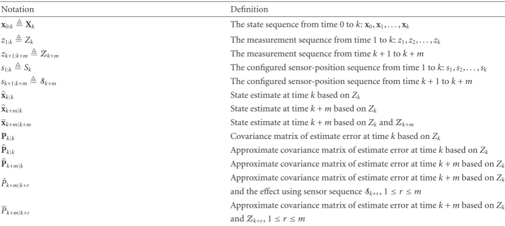
This paper is organized as follows. InSection 2, we for-mulate the tracking scenario and describe the tracking algo-rithm. InSection 3, we present the optimization framework for sensor scheduling, and propose the two sensor scheduling algorithms for nonmyopic scheduling. InSection 4, we dis-cuss the two optimal pruning algorithms, and inSection 5, we demonstrate the improved performance of our algo-rithms using Monte Carlo methods. Note that our adopted notation is summarized inTable 1.
2. TARGET TRACKING SCENARIO
For the sake of concreteness, we formulate the sensor sched-uling problem in the context of a scenario in which an acous-tic homing torpedo tracks a surface target (Figure 1) [15]. Note however, that our scheduling algorithms can be readily adapted to other problems with discrete configuration op-tions including tracking an airborne target with a missile or optimizing the tracking performance in a network of sensors where the target belief transfer (between two sensors) is con-strained by network energy and bandwidth costs [16].
2.1. Problem formulation
We consider a target moving in two-dimensions. The target state at timek is xk = xk x˙k yk y˙kT, where xk and yk represent the target position in Cartesian coordinates, and ˙xk and ˙yk represent the corresponding velocity. We model the target dynamics with a constant-velocity model given by
xk=Fxk−1+wk−1. (1)
Here,Fis the state transition matrix, andwkis a zero-mean white Gaussian sequence with covarianceQ.
At each timek, the torpedo’s acoustic sensors obtain the noisy bearing measurementzk:
zk=h
xk;xs k,yks
+vktan−1 y
k−ysk xk−xsk
+vk, (2)
wherevkis zero-mean white Gaussian noise with varianceσ2, xs
Table1: Adopted notation.
Notation Definition
x0:kXk The state sequence from time 0 tok:x0,x1,. . .,xk
z1:kZk The measurement sequence from time 1 tok:z1,z2,. . .,zk
zk+1:k+mZk+m The measurement sequence from timek+ 1 tok+m
s1:kSk The configured sensor-position sequence from time 1 tok:s1,s2,. . .,sk
sk+1:k+mSk+m The configured sensor-position sequence from timek+ 1 tok+m
xk|k State estimate at timekbased onZk
xk+m|k State estimate at timek+mbased onZk
xk+m|k+m State estimate at timek+mbased onZkandZk+m
Pk|k Covariance matrix of estimate error at timekbased onZk
Pk|k Approximate covariance matrix of estimate error at timekbased onZk
Pk+m|k Approximate covariance matrix of estimate error at timek+mbased onZk
ˇ
Pk+m|k+r Approximate covariance matrix of estimate error at timek+mbased onZk
and the effect using sensor sequenceSk+r, 1≤r≤m
Pk+m|k+r Approximate covariance matrix of estimate error at timek+mbased onZk
andZk+r, 1≤r≤m
(0, 0)
x y
Available torpedo maneuvering options
Ë
Torpedo
bmeters Current sensor
direction
Target trajectory Target
Figure1: Tracking scenario: a sea target is tracked by a torpedo. At each time epoch, the torpedo can change heading by one of nine possible values and then movebmeters.
At a given timek, the torpedo can change heading by one of the nine possible values{iπ/16,i= −4,. . ., 4}as shown in Figure 1; it then movesbmeters along its new heading. These possible torpedo motions define the set of possible sensor configuration options for this problem; in the following, we will refer to these as sensor motion or sensor configuration options.
We denote the configured sensor position at timek by sk (xsk,yks), and the sequence of positions from 1 tokby Sks1:k. The sensor configuration atkis denoted bygk. We
denote the set of allowable sensor configurations as Gand the number of configurations asU. For example, inFigure 1,
there areU=9 allowable sensor configurations at each time k: move along the current heading or change to one of eight possible new directions. The configured sensor positionsk+1
at timek+ 1 is a deterministic function ofgk+1 andsk; we
assume that there is no uncertainty or error in the sensor movement. Thus, given the initial sensor positions0and the
sequence of sensor configurationsg1,. . .,gk, we can obtain
the configured sensor positionskat timek.
2.2. Target tracking using a particle filter
The extended Kalman filter is often not robust in bearing-only tracking because of target observability problems; for this reason, we use a particle filter to track the target [17]. In a particle filter, the posterior probability densityp(xk|Zk,Sk) is approximated byNparticlesxi
kand associated importance weightswik,i=1,. . .,N, asp(xk |Zk,Sk)≈
N
i=1wikδ(xk− xki). The minimum mean-square error (MMSE) estimate of the target state is the mean xk|k = Exk|Zk,Sk[xk | Zk,Sk] ≈
N
i=1wkixki of this density, whereE[·] denotes expectation;1 the covariance matrix of the estimate error is approximated asPk |k≈ Ni=1wik(xki −xk|k)(xik−xk|k)T.
At each timek, the particlesxki are drawn from the prior density p(xk | xk−1); after obtaining a measurement zk,
the weights are updated recursively usingwik =wki−1p(zk | xki,sk)/( Nj=1w
j
k−1p(zk|xkj,sk)). Resampling is performed to avoid degeneracy of the particles [17].
3. NONMYOPIC SENSOR SCHEDULING
Nonmyopic scheduling is important when myopic deci-sions result in poor estimation performance. In the current
1Note that when necessary, we use the notationEx[·] to clarify that the
tracking scenario, the need for nonmyopic scheduling arises due to the constrained maneuverability of the sensor. Non-myopic sensor scheduling can be realized in two ways. The first is open-loop (OL) scheduling, in which the scheduling is performed only after all multistep decisions are exhausted [18]. The second is open-loop feedback (OLF) scheduling, in which only the first scheduling decision is executed, and the nonmyopic scheduling is repeated at each time step [18– 22]. Although our algorithm description is based on OL scheduling, the optimization framework for both scheduling schemes is the same [18]. We will demonstrate through our results that OLF scheduling is better than OL scheduling due to the feedback obtained in scheduling decisions at each time step. Next, we describe the optimization framework before presenting our new sensor scheduling algorithms.
3.1. Optimization framework
Following the scenario inFigure 1, the sensor can be config-ured inUdistinct ways at each time stepk. At any given time k, our objective is to obtain the best sensor-configuration se-quence over the nextMtime-steps in order to minimize the scheduler cost. We denote a sensor-configuration sequence by anM-tuple:Sk+M
sk+1 sk+2 · · · sk+M T
, wheresk+m is the configured sensor position at timek+m(msteps in the future). Note that there is a total ofUM distinct sensor sequences of lengthM.
We denote the scheduler cost at timek+mbyJ(sk+m).
We define the total scheduler cost for a particular sensor se-quenceSk+Mas
JSk+M
=
M
m=1
Jsk+m
. (3)
We seek the optimal sequenceSoptk+Mthat minimizesJ(Sk+M):
Sopt
k+M=arg minS k+M
JSk+M
. (4)
Equation (4) is a discrete optimization problem, where the scheduler cost is optimized over the finite set of possible sen-sor sequences. Note that our rationale for using the additive scheduler-cost structure2in (3) is that the costs in this paper
are both stochastic and predictive; the scheduler costs are ob-tained by computing an expectation over the predicted state distribution. AsMincreases, the accuracy with which track-ing performance can be predicted decreases. Thus, we do not rely only on the terminal cost of a sensor sequence, but also on the costs at intermediate points in time.
We consider two different scheduler costsJ(sk+m) in this
paper. The first is the determinant of the predicted state
2Note that in the current application scenario, both additive
scheduler-cost in (3) and terminal scheduler-cost (in which we minimizeJ(Sk+M) to obtain the best sensor sequence) resulted in similar tracking performance.
estimate error covariance matrix at timek+m. Specifically withZk+mzk+1:k+m,
Jsk+m
=Psk+m
=Exk+m,Zk+m
xk+m−xk+m|k+m
xk+m−xk+m|k+m T
. (5)
Minimizing this cost implies reducing the volume of the co-variance ellipsoid [23].
The second cost is the Kullback-Leibler (KL) distance be-tween the approximate predicted and filtered state densities. This is an information-theoretic metric that can be used to measure the average information gain in using each sensing action [24–26]. The KL distance cost is defined asJ(sk+m)=
EZk+m|sk+m[C(Zk+m,sk+m)], whereC(Zk+m,sk+m) is a condi-tional cost function [27]:
CZk+m,sk+m
= −
xk+m
pxk+m|Zk+m,Sk+m
×log
pxk+m|Zk+m,Sk+m
pxk+m|Zk+m−1,Sk+m−1
dxk+m. (6)
Here, p(xk+m | Zk+m−1,Sk+m−1) and p(xk+m | Zk+m,Sk+m)
are approximations of the predicted and filtered densities at time k+m. Note the negative sign in (6); minimizing the conditional cost maximizes the KL distance, as desired.
The determinant cost approximates the target uncer-tainty using only the first- and second-order statistics of the posterior distribution. This cost can be approximately com-puted efficiently using the recursive Riccati equation, as im-plemented by the CB algorithm in Section 3.2.1. The KL distance cost depends on the entire posterior distribution and directly measures the average information contributed by each sensor configuration about the target state. How-ever, the KL distance cost is computationally more expensive than the determinant cost as the KL distance cost cannot be computed using closed-form Riccati-like recursive formula-tions.
3.2. Proposed nonmyopic scheduling algorithms
We propose two nonmyopic sensor scheduling algorithms: the CB algorithm and the UTB algorithm. Both algorithms find the optimal sequence of sensor uses by searching ex-haustively over all possible sequences. In principle, this re-quires the computation ofJ(Sk+m) for each possible sequence
Sk+m. We note that for any two sequences,Sk1+m+1andSk2+m+1
(1≤m < M), that have the same initial subsequenceSk+m,
the computation ofJ(Sk+m) is redundant when concurrently
computingJ(S1
For each possible sequence of sensorsSk+M=sk+1:k+M
(1) Initialize:xk|k= Ni=1wkixik, ˇPk|k=Pk|k= i=N1wik(xki−xk|k)(xki−xk|k)T
(2) Form=1 toM,
– Project the state estimate and covariance matrix of estimate error:
(i)
xk+m|k=Fxk+m−1|k (7)
(ii)
ˇ
Pk+m|k+m−1=FPˇk+m−1|k+m−1FT+Q (8) – Compute the Jacobian matrixHk+m:
(iii)
Hk+m=
∂θ ∂x
∂θ ∂x˙
∂θ ∂y
∂θ ∂y˙
T
x=xk+m|k
whereθ=hx;xs,ys (9)
– Update the predicted covariance matrix of estimate error:
(iv)
ˇ
Pk+m|k+m=
ˇ P−1
k+m|k+m−1+ 1
σ2Hk+mH T k+m
−1
(10)
– CalculateJ(sk+m)= |Pˇk+m|k+m| End
(3) CalculateJ(Sk+M) using (3)
End
Choose the optimal sequence of sensors using (4)
Algorithm1: The CB algorithm.
be easily eliminated in the actual implementation of the al-gorithm.
3.2.1. Covariance-based sensor scheduling
The covariance-based (CB) sensor scheduling algorithm uses the covariance-based cost and is particularly well-suited for tracking systems with limited computational and memory resources [28]. Specifically, the computational complexity of the CB algorithm in obtainingJ(sk+m) for a givensk+m is in the order ofO(n3
x), wherenxis the dimension ofxk.
In the CB algorithm, we approximate P(sk+m) in (5) by linearizing the measurement model in (2) about a pre-dicted target state xk+m|k; we denote this approximation by ˇPk+m|k+m. Our iterative CB algorithm is summarized in
Algorithm 1. It is initialized by the estimatesxk|k andPk |k computed at timekby a particle filter (inSection 2.2). For each sequence Sk+m, equations (i) and (ii) ofAlgorithm 1
are used to predict xk+m|k and ˇPk+m|k+m−1 to time k+m;
we then linearizeh(x;xs,ys) aboutxk
+m|kto compute the Ja-cobian matrix Hk+m in equation (iii). ˇPk+m|k+m is obtained using equation (iv) inAlgorithm 1; the determinant sched-uler cost is then obtained as J(sk+m) = |Pkˇ +m|k+m|. Finally, J(Sk+M) is obtained using (3). Note that equations (i) and
(ii) of Algorithm 1 correspond to the prediction step of the extended Kalman filter (EKF), while equation (iv) of Algorithm 1corresponds to the update step of the EKF.
The CB is similar to the PCRLB algorithm in [8], but was developed independently [28]. The two algorithms differ in the calculation of the sensor information term, that is, (1/σ2)Hk
+mHTk+m; while the CB algorithm computes it us-ing the predicted state estimatexk+m|k, the PCRLB algorithm computes an expected value of the sensor information term using the predicted state densityp(xk+m|Zk,Sk).
3.2.2. Unscented transform-based sensor scheduling
The motivation for the unscented transform-based (UTB) algorithm is to provide a generalized framework that al-lows sensor scheduling using information-theoretic costs. The UTB algorithm does not require the Jacobian matrix; this is useful when it is not possible to obtain the Jacobian matrix analytically. For instance, in a tracking scenario where the measurements are binary valued (detect or no-detect) and depend probabilistically on the state (e.g., through a probability of detection), it is not possible to obtain an ex-pression of the Jacobian matrix.
xkD+1,l xDk+2,l xkD+3,l Dk+1 Dk+2 Dk+3
wkj,+1l wkj+2,l wkj,+3l zkC+1,j zCk+2,j zkC+3,j
Ck+1 Ck+2 Ck+3
xkB+1,ζ xBk+2,ζ xkB+3,ζ xAk,i
Bk+1 Bk+2 Bk+3
Ak
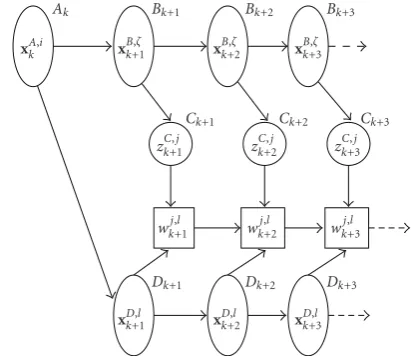
Figure2: Sets of particles used to compute the expected future cost for the UTB algorithm.
Grid-based sampling techniques as used in [25,29] are also computationally expensive as they require large number of particles to compute expected scheduler costs. Instead, we propose in this paper to use the unscented transform (UT) to generate future particles [30]. As these sample particles are few in number, the computational load in calculating the scheduler costs is significantly reduced.
The UTB algorithm is summarized in Algorithm 2. In this algorithm, we use several sets of particles as shown in Figure 2. At time k+m, the particle sets used areBk+m =
{xkB+,ζm},ζ = 1,. . .,Nσ, which is a predicted set of Nσ state particles calculated using the UT (whereNσ is the number of sigma points obtained using the UT) and approximates p(xk+m | xk,Sk);Cksk++mm = {z
C,j
k+m}, j = 1,. . .,E, which is a predicted set of E measurement3 particles calculated using
theNσ state particles and approximates p(zk+m | xk,sk+m);
andDk+m = {xkD+,lm},l=1,. . .,L, which is a predicted set of L(≤ N) state particles and approximates p(xk+m | xk,Sk). Also,XDk+,lm xkD+1,l · · · xkD+,lmT,l=1,. . .,L, andZCk+,jm
zkC+1,j · · · z
C,j k+m
T
, j = 1,. . .,E, are defined as thelth pre-dicted state sequence and thejth predicted measurement se-quence, respectively, from timek+ 1 tok+m. We now de-scribe theM-step UTB algorithm.
InitializeAk= {xAk,i},i=1,. . .,N, as the set of resampled particles computed by the particle filter at timek.
InitializeDk+1 = {xkD+1,l},l=1,. . .,L, by randomly
sam-plingLparticles from the setAk, and predicting these parti-cles tok+ 1 by sampling from the distributionp(xk+1|xAk,l). Initialize the setBk+1 = {xkB+1,ζ},ζ =1,. . .,Nσ, by
perform-ing a UT on the setAk through the steps (i) to (iii) in the following.
3We uses
k+mas a superscript inCksk++mmto denote the explicit dependence of the measurement set on the sensorsk+m.
(i) Compute the predicted mean and predicted covari-ance matrix of estimate error at timek:
xk|k= 1 N
N
i=1
xAk,i,
Pk|k=1 N
N
i=1
xkA,i−xk|k
xAk,i−xk|k T
.
(15)
(ii) Definexa k|k =
xTk|k 0 0T as a concatenation of the state, process noise, and measurement noise vectors, andPak|k = diag(Pk|k,Q,σ2) as the covariance ofxak|k. The length of the vectorxak|kis denoted byna=9. (iii) Using the UT [31], we deterministically computeNσ =
2na+ 1 sigma points fromAk. The sigma points are defined asXζk
Xkx,ζ Xwk,ζ Xkv,ζT,ζ = 1,. . .,Nσ, and are computed as [31]
Xζk= ⎧ ⎪ ⎪ ⎪ ⎪ ⎪ ⎪ ⎪ ⎨ ⎪ ⎪ ⎪ ⎪ ⎪ ⎪ ⎪ ⎩
xak|k, ζ=0,
xak|k+Λζ, ζ=1,. . .,Nσ−1 2 ,
xak|k−Λζ−na, ζ= Nσ+ 1
2 ,. . .,Nσ.
(16)
Here Xxk,ζ, X
w,ζ
k , and X
v,ζ
k denote the partition of Xζk in the target-state space, process-noise space, and measurement-noise space, respectively. Furthermore,
Λζis theζth column ofΛ,Λ=
(na+λ)Pak|k, andλ= a20(na+κ)−na. Note that 0≤a0≤1 determines the
spread of the sigma points around xak|k. A value of a0 =0.1 was chosen through experimentation to
en-sure that the sigma points are neither spaced too far from the mean nor too close to the mean. The sec-ondary scaling parameterκis generally set to zero [31]. Now, using the sigma points, we calculate the elements of the setsBk+1asxkB+1,ζ =FX
x,ζ k +X
w,ζ
k ,ζ=1,. . .,Nσ. We then iterate the following steps form=1 toM.
Step 1. Form > 1, obtain the elements ofDk+m asxDk+,lm = FxDk+,lm−1+ξD,l = 1,. . .,L, whereξD is a random sample drawn from a Gaussian distribution of zero mean and co-varianceQ.
Step 2. Form > 1, obtain the elements ofBk+masxBk+,ζm = FxBk+,ζm−1+ξB,ζ = 1,. . .,Nσ, whereξBis a random sample drawn from a Gaussian distribution of zero mean and co-varianceQ.
Step 3. Obtainηmeasurements for each sigma point inBk+m using the distribution p(zk+m | Xxk+,ζm−1,sk+m) to form the measurement setCsk+m
k+m withE = ηNσ measurement parti-cles.
Step 4. Using the setsCsk+m
k+mandDk+m, we compute the
For each possible sequence of sensorsSk+M
(1) Initialize:Ak,Bk+1andDk+1 (2) Form=1 toM,
– Obtain setsBk+m,Cksk++mm, andDk+musing Steps1–3inSection 3.2.2
– Compute the costJ(sk+m):
(i) Computewkj,+lmusing the particles inDk+mandCksk++mm:
wkj,+lm∝pzkj+m|xl k+m,sk+m
pZkj+m−1|Xlk+m−1,Sk+m−1
(11)
(ii) Compute the approximate conditional cost functionC(Zk(+j)m,sk+m) in (17) and (18) usingwkj,+lmandxlk+m.
(iii) Compute the approximate conditional density ofZkj+musingDk+m:
pZkj+m|Zk,Sk+m
≈ L
l=1
pZkj+m|xl k+m,Sk+m
= L
l=1
pzkj+m|xl k+m,sk+m
pZkj+m−1|Xlk+m−1,Sk+m−1
(12)
(iv) Compute the expectation ofC(Zkj+m,sk+m) at timek+mas
EZk+m
CZj k+m,sk+m
≈
E j=1γ
j k+mC
Zkj+m,sk+m
E j=1γ
j k+m
, whereγkj+mp
Zkj+m|Zk,Sk+m
(13)
(v) Compute the scheduler cost at timek+mas
Jsk+m
= ⎧ ⎨ ⎩
EZk+m
CZj
k+m,sk+m for KL cost P
sk+mEZk+m
CZj
k+m,sk+m for determinant cost.
(14)
(3) Calculate the total scheduler cost using (3)
End
Choose the optimal sequence of sensors using (4)
Algorithm2: The UTB algorithm.
in Algorithm 2. We then obtain the total scheduling cost J(Sk+m) using (3); optimizing over all sequences gives the
op-timal sensor sequenceSkopt+musing (4). Note that when possi-ble inAlgorithm 2and hereafter, we drop the superscriptC fromZCk+,jmand the subscriptDfromXkD+,lmandxDk+,lm, to sim-plify the notation.
The method inAlgorithm 2can be used for any condi-tional cost function that depends on future measurements. The conditional cost function for covariance-based costs is given as
CCOV
Zj
k+m,sk+m
=
L
l=1
wkj,+lm
xlk+m−xkj+mxlk+m−xkj+mT, (17)
wherexkj+m = L l=1w
j,l
k+mxlk+m, andw j,l
k+mare the weights ob-tained in step (ii) ofAlgorithm 2.
For the KL distance cost, the corresponding conditional cost is derived inAppendix A, and is given by
CKL
Zj
k+m,sk+m
=
L
l=1
−wkj,+lmlog ⎡ ⎣ wkj,+lm
wkj,+lm−1
⎤
⎦. (18)
Equation (18) resembles the KL distance between two dis-crete distributions and can be interpreted in a similar way. The particles in set D each has weights equal to wkj,+lm−1,
and represent our belief of the future state. Each predicted measurement zkj+m updates these weights to w
j,l
k+m, accord-ing to the measurement model. The gain in information for each predicted measurement is calculated using (18), which is then averaged with respect to the measurement density p(Zkj+m|Zk,Sk+m).
k+ 3
k+ 2
k+ 1
k
M=3
Figure3: An illustrative configuration tree withU=4 configura-tion choices and a time horizon ofM=3.
predicted measurementszkj+mon the predicted density func-tion p(xk+m | Zkj+m−1,Sk+m−1). AlthoughL andE are
re-quired to be large numbers in order to accurately predict the scheduler costs, this results in a significant increase in com-putational complexity. Furthermore, as we are mainly inter-ested in the relative tracking performance achievable with the available sensor configurations, we can trade offthe compu-tational cost of scheduling with the accuracy of the predicted tracking performance. To this effect, we chooseL=2000 and E=380 (η=20) for the state and measurement particles.
We further note that in order to compute wkj,+lm, we need to store p(Zkj+m−1 | Xl
k+m−1,Sk+m−1) (equation (i) of
Algorithm 2) in memory and access it only when required. However, as storing p(Zkj+m−1 | Xl
k+m−1,Sk+m−1) requires
a lot of memory, in this work the scheduler stores only the predicted measurements for each sensor configuration. We note that p(Zkj+m−1 | Xl
k+m−1,Sk+m−1) is generated only
once when concurrently computing J(sk+m) for two sensor
sequences having identical measurement history up to time k+m−1.
The computational complexity of the UTB algorithm in obtainingJ(sk+m) with the KL cost for a givensk+m is in the order ofO(nxEL); thus, the UTB algorithm is computation-ally more expensive than the CB algorithm. Furthermore, the computational complexity in obtainingP(sk+m) for the determinant cost in equation (v) ofAlgorithm 2, given the weightswkj,+lm andγkj+m (in equations (i) and (iv), resp., of Algorithm 2), is in the order ofO(nx(nx+ 2)EL). An alterna-tive formulation in obtainingP(sk+m) is
Psk+m
=P1
sk+m
−P2
sk+m
, (19)
whereP1(sk+m) = Ll=1wlk+m(xlk+m−xk+m)(xlk+m −xk+m)T
with
xk+m= L
l=1
wl k+mxlk+m,
wlk+m= E j=1p
zkj+m|xlk+m,sk+m
pZkj+m−1|Xl
k+m−1,Sk+m−1
E
j=1 Ll=1p
zkj+m|xlk+m,sk+m
pZkj+m−1|Xl
k+m−1,Sk+m−1
, l=1,. . .,L,
P2
sk+m
=
E j=1γ
j k+m
xkj+m−xk+m
xkj+m−xk+m T
E j=1γ
j k+m
.
(20)
This formulation avoids computing CCOV(Zkj+m,sk+m)
(in (17))Etimes for equation (ii) inAlgorithm 2, and it re-duces the computational complexity in obtainingP(sk+m) to
the order ofO(nxEL), that is, by an order ofnx+ 2=6.
4. PRUNING ALGORITHMS FOR NONMYOPIC
SENSOR SCHEDULING
4.1. Tree search and pruning algorithms
The sensor sequences (of lengthM) can be arranged in a tree of depthMas shown inFigure 3, with each depth-mnode of the tree depicting a configured sensor position at timek+m. Thus, the sensor scheduling problem can be posed as a tree search problem, where the best sensor sequence corresponds to the lowest-cost branch of this tree.
We use the following terminology. A node isopenif its cost has been computed,expandedif all its children have been
opened, andprunedif the node and its children have been re-moved from the tree. Note that during a node expansion, we compute the cost of all of the children nodes. Pruning a node with optimality means that the pruned node is guaranteed not to be a part of the best sensor sequence.
Initialize: SolutionFound=FALSE and list=root node
While(SolutionFound=FALSE) and (there is a node in the list)
Remove the first node from the list and expand it
Ifdepth of children nodes=M
Sort the children nodes in ascending order of costs Append the sorted children nodes to the list
else
Ifsolution is found
Set SolutionFound=TRUE
End end end
Algorithm3: Pseudocode for breadth-first search.
In the UCS, the lowest-cost unexpanded node of a tree is expanded regardless of its depth in the tree [11]. The pseu-docode for UCS is exactly the same as that for BFS, except that instead of appending the sorted children nodes to the list, we insert the children nodes into the list such that the updated list is in ascending order of cost. UCS is more time-efficient than BFS, but has the same memory complexity as BFS [11].
GS always expands the lowest-cost, lowest-depth, open node of the tree;Algorithm 4shows its pseudocode. GS ex-pands only the lowest-cost open node at each depth of the tree, so its memory and time complexity isO(UM). GS does not search the tree exhaustively and does not guarantee the optimal solution.
With exhaustive search, a total ofUM sensor sequences must be considered to obtain the optimal sensor sequence. AsMincreases, the number of sensor sequences grows expo-nentially; since the computational time and memory usage increase exponentially as well, it is imperative to reduce the search space as much as possible. We propose two optimal pruning algorithms that significantly reduce the computa-tional burden in obtaining the sensor sequences. The prun-ing algorithms are optimal as they provide the same best sen-sor sequence as the one obtained using an exhaustive search [32].
These pruning algorithms use the branch-and-bound technique; the B&B technique is often used to prune the search tree for problems such as the traveling-salesman prob-lem, vehicle routing, and production planning [33,34]. Ap-plication of this technique requires that lower bounds on the costs of all nodes in the tree are easier to compute than the actual costs of the nodes. Typically, in a B&B aided tree search, the tree is traversed using a search technique with de-sired time/memory tradeoffs; whenever a potential best so-lution is obtained, its cost is compared to the lower bounds of all the unexpanded open nodes. Any node whose lower bound is larger than the cost of the current best solution is pruned from the tree. B&B can significantly reduce the computational and memory requirements but typically does not eliminate exponential complexity. As part of our future work, we will investigate efficient search algorithms that do not require a complete enumeration of the search space.
Initialize: SolutionFound=FALSE and list=root node
While(SolutionFound=FALSE) and (there is a node in the list)
Expand the first node and remove it from the list
Ifdepth of children nodes=M
Sort the children nodes in an ascending order of costs Prepend the list with sorted children nodes
else
Choose lowest cost depthMopen node as the best solution
Set SolutionFound=TRUE
end end
Algorithm4: Pseudocode for greedy search.
4.2. Branch-and-bound-based pruning algorithms
We present two B&B based pruning algorithms in this sec-tion. The first pruning algorithm that we developed com-bines BFS and GS with the B&B technique, and is relatively efficient in memory usage. We call this the BFS-GS pruning algorithm. The second pruning algorithm is referred to as a best-first B&B algorithm [35] in the literature; it combines UCS with the B&B technique and is relatively efficient in pro-cessing time.
The pruning algorithms address two main issues of an exhaustive search: (a) each node expansion requires compu-tation of the scheduler cost since the costs are stochastic in nature and are not known a priori, and (b) each open node (except depth-M nodes) requires memory to store the pre-dicted state information. Specifically, for the CB algorithm, each node stores a mean vector and a covariance matrix, while for the UTB algorithm, each node stores a set of mea-surement particles. Additionally for each node, its cost, its status (open, close, or pruned), and an index to identify its position in the tree must be stored.
In simulations, we observed that the cost of some depth Mnodes that resulted in improved tracking performance was lower than the cost of many intermediate depth nodes that resulted in poor performance. Furthermore, it was found that suboptimal techniques that accept the first candidate so-lution found (such as a pure GS or a combination of BFS and pure GS) yield poor tracking performance in compari-son to an optimal search. This motivated us to use the B&B framework. The additive cost in (3) guarantees that for non-negative scheduler costs, any children of these poor perfor-mance intermediate depth nodes will have larger costs than the depthM nodes. Making use of this fact, we assign the lower bound on the cost of any unopened node as the cost of its nearest open ancestor. Specifically, for a given sensor sequenceSk+m withm > 1, the lower bound onJ(sk+m) is
chosen asJ(sk+r), wheresk+r (1 ≤ r < m) corresponds to the deepest open node inSk+m. This bound is a valid lower
bound because the additive cost structure in (3) guarantees thatJ(sk+r)≤J(sk+m) forr < m. Although this bound is
Initialize: cmin= ∞
Perform BFS up to depthdint< M
Store the depthdintnodes in a list, sorted in ascending order of cost
Whilethere is a node in the list
Expand the first node and remove it from the list
Ifdepth of children nodes=M
Ifthe lowest-cost child node has cost lower thancmin Setcminto this cost
Set BestNode to this child
end else
Sort the children nodes in ascending order of costs Prepend the list with sorted children nodes
end
For all nodes in the list
Ifcost of a node≥cmin remove the node from the list
end end
Trace back the BestNode to the root node to obtainSkopt+M
Algorithm5: Pseudocode for the BFS-GS pruning algorithm.
It must be noted that our B&B algorithms are applica-ble only with positive scheduler costs (e.g., determinant and trace of covariance matrix of estimate error, and entropy of the posterior distribution). Since the KL distance cost in (18) is negative, our B&B pruning algorithms cannot be used with the KL-based scheduling.
We now present our two pruning algorithms.
4.2.1. BFS-GS pruning algorithm
The pseudocode for our proposed BFS-GS pruning algo-rithm is provided inAlgorithm 5. In this algorithm, we first perform a BFS to an intermediate depth dint, and then
be-ginning with the best node of depthdint, we perform a GS
to the terminating depthM. The GS gives an initial candi-date path ending in a node with cost that we denotecmin.
We then repeat the following until there are no unexpanded open nodes.
Step 1. Compare the cost of all unexpanded open nodes to cmin; prune any node whose cost is not less thancmin. The
additive cost guarantees that the best node cannot be a child of any pruned node.
Step 2. Perform a GS on the tree beginning at the lowest-cost open node; at each expansion compare the lowest-cost of the children nodes withcmin and prune away the nodes whose
cost is not less thancmin. If the GS gives a path with a terminal
node whose cost is less thancmin, setcminto be this cost and
the best path to be this path.
The intermediate depth dint is an important factor for
the BFS-GS pruning algorithm since the best node at this depth is used as a starting point for the GS to find an initial
candidate solution. Asdint increases, the probability of the
initial candidate solution being closer to the best solution in-creases. However, large values ofdintare undesirable because
an exhaustive-search (here BFS) to depthdintis conducted.
At the same time, a small dint is undesirable as the initial candidate solutions obtained using it are often of poor qual-ity, which results in superfluous expansion of nodes. For the problem under consideration, we found that a good compro-mise for the BFS-GS algorithm isdint= M/2 .
4.2.2. UCS pruning algorithm
The second pruning algorithm combines UCS with the B&B algorithm. In this algorithm, we first use a UCS to expand the nodes until the terminating depthMis reached. The lowest cost sensor sequence of lengthMis used as an initial candi-date solution whose cost is denoted bycmin. We then repeat
the same two steps of the BFS-GS pruning algorithm, except that we use a UCS instead of the GS. The pseudocode for this algorithm is the same as that inAlgorithm 5, except that we set dint = 1 and instead of sorting the children nodes and
adding them to the front of the list, we insert the children nodes in the list such that the updated list is maintained in ascending order of costs.
4.3. -suboptimal search
We may significantly reduce the computational effort of find-ing a sensor sequence if we relax the requirement of optimal-ity. Using an-suboptimal search, it is possible to find a good sequence that does not significantly increase the scheduler cost. The costcsubobtained by an-suboptimal search always
satisfiescsub< cbest(1+), wherecbestis the cost of the optimal
sequence. In our pruning algorithm, the-suboptimal search is implemented by dividingcminby 1+, and using the
result-ing value to prune the sensor sequences. This is equivalent to making the lower bound of the nodes tighter by a factor of 1 +. We found through simulations that 0< <0.2 is an acceptable choice, and that for these values, the increase in cost over the optimal solution is approximately 35% (e.g., =0.2 generally gives a solution within 7% of the optimal cost).
5. SIMULATIONS AND RESULTS
We used Monte Carlo (MC) simulations to evaluate the per-formance of the sensor scheduling algorithms for the tar-get/torpedo scenario described inSection 2.1. The initial tar-get position and velocity are (x,y) = (2000, 2500) m and ( ˙x, ˙y)=(−4.5,−4.5) m/s, respectively; the average speed of the target corresponds to 6.36 m/s (12.18 knots). The tar-get travels for 40 time-steps of one second each, and a sin-gle bearing measurement is obtained in each time step; the standard deviation of the measurement error is 0.035 radi-ans (2◦). The torpedo and its sensor are initially located at (2100, 2300) m and moveb=15 m in each one-second time step (a speed of 28.73 knots).
0 5 10 15 20 25 30 35 40 Time index (k)
0 5 10 15 20 25 30 35
RMSE
(m)
M=1
M=2
M=3
M=4
M=5 (a)
1800 1850 1900 1950 2000 2050 2100 2150
x(m) 2250
2300 2350 2400 2450 2500 2550
y
(m)
End Initial sensorlocation
Target trajectory
M=2
M=4
(b)
Figure4: (a) Comparison of the RMSE of the target position estimate forM=1, 2,. . ., 5 OL scheduling using the UTB algorithm with the determinant cost. (b) Comparison of the sensor trajectories for theM=2 andM =4 OL scheduling using the UTB algorithm with the determinant cost.
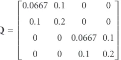
increase in N does not bring a significant improvement in the tracking performance. The particles were initialized us-ing a Gaussian density whose mean was the true target state and whose covariance was diag(500 10 500 10). The pro-cess covariance matrix in (1) was chosen as
Q=
⎡ ⎢ ⎢ ⎢ ⎢ ⎢ ⎢ ⎣
0.0667 0.1 0 0 0.1 0.2 0 0 0 0 0.0667 0.1 0 0 0.1 0.2 ⎤ ⎥ ⎥ ⎥ ⎥ ⎥ ⎥ ⎦
. (21)
Also, 100 MC simulations were performed for each set of pa-rameter values.
5.1. Nonmyopic scheduling results
5.1.1. Open-loop scheduling
In this simulation, we investigated the performance of OL scheduling for values ofMfrom 1 to 5; nonmyopic schedul-ing provided improved performance. We used the UTB algo-rithm with the determinant cost to obtain the sensor con-figuration sequence. The UTB parameters were chosen as L=2000,a0=0.1,κ=0, andη=20 (refer toSection 3.2.2).
Figure 4(a)compares root mean-square error (RMSE) of the target position forM = 1,. . ., 5. It can be seen that as Mincreases, the RMSE performance improves, and it begins to saturate with increasingM. The RMSE curve forM =4 step scheduling is on an average 2 m higher than that for the M=5 step scheduling, but has a much lower computational cost; we can conclude that for the current tracking scenario, M=4 step scheduling may suffice.
Figure 4(b)compares the sensor trajectory of one of the MC runs forM = 2 andM = 4 step scheduling. Initially, the sensor trajectory is similar; both schedulers use the same trajectory to reduce the initial high uncertainty about the tar-get position. After about 16 s, the trajectories begin to differ. WhenM=4, the sensor remains in the vicinity of the target; however, whenM = 2, the sensor cannot plan far enough ahead to maintain a close proximity to the target. This is due to the constrained sensor movement, which leads to poor RMSE tracking performance in comparison to the case with M=4.
We also performed scheduling with the KL distance cost forM = 1,. . ., 3 using the UTB algorithm. Figure 5 com-pares the RMSE results (marked as KLM = 1,. . ., 3); the RMSE performance improves with increasingM. For com-parisons, we also include the RMSE result obtained with the determinant cost with M = 3 (labeled as Det M = 3). The KL scheduling resulted in slightly better RMSE perfor-mance than the determinant cost. This is possibly because the KL scheduling uses the complete statistics of the predicted state densities, while the determinant scheduling uses only up to second-order statistics (through the predicted covari-ance matrix).
5.1.2. Open-loop feedback scheduling
0 5 10 15 20 25 30 35 40 Time index (k)
5 10 15 20 25 30 35
RMSE
(m)
KLM=1 KLM=2
KLM=3 DetM=3
Figure5: Comparison of the RMSE of the target position estimate forM =1, 2, and 3 with the KL distance cost, using the UTB al-gorithm. TheM=3 case with the determinant cost is included for comparison.
OLF scheduling forM =2, 3, and 4. It can be seen that the OLF scheduling performs better in all the cases. This is be-cause OLF improves its scheduling decisions using the feed-back provided by the measurement at each time-step. This however results in a higher computational cost (than the OL scheduling) asM-step scheduling is performed at each time-step.
5.2. Comparisons of UTB and CB scheduling
Next, we compare the UTB and CB OL scheduling results for the tracking example with the determinant cost.Figure 7 compares the RMSE performance for the CB and UTB algo-rithms forM =3 andM = 4. It can be seen that the UTB algorithm yields slightly better RMSE performance than the CB algorithm. For example, whenM =4, the RMSE curve for the UTB algorithm is on an average 2 m lower than the RMSE curve for the CB algorithm. However, the CB algo-rithm is computationally more efficient than the UTB al-gorithm. For instance, on a Pentium IV 2.4 GHz computer with Matlab software, an exhaustive search forM =3 step scheduling requires 236 s with the UTB algorithm, but only 9 s with the CB algorithm. Further, the CB algorithm requires 56 bytes for each node to store a mean and covariance while the UTB algorithm requires 1.52 KB for each node to store the measurement set C. The reduced processing-time and memory requirements make the CB algorithm a better choice for computationally constrained tracking systems.
5.3. Pruning results
We conducted three sets of Monte Carlo experiments to eval-uate the effectiveness of pruning in reducing the scheduling computational load. The first set of experiments investigated
whether the optimal sensor sequence performs significantly better in terms of scheduler cost than sequences found us-ing a suboptimal heuristic search technique; we found the optimal sequence to be significantly better. The second set of experiments investigated the relative computational re-quirements of the BFS-GS and UCS B&B algorithms. The third set of experiments investigated the tracking perfor-mance/computation tradeoffs of the-suboptimal search.
5.3.1. Comparison of suboptimal heuristic
and optimal algorithms
In order to assess the tracking performance of suboptimal search, we first compare the tracking performance ofM=4 OL optimal scheduling with the tracking performance of M=4 OL suboptimal scheduling using the following heuris-tic: the first candidate solution obtained with a BFS up to depthd1is the starting point for a pure GS from depthd1to
depthM=4. We use the abbreviation Sub[d1,M] to denote
this search.Figure 8(a) compares the results obtained with Sub[1, 4], Sub[2, 4], and Sub[3, 4], and the optimalM = 4 scheduling. We note that the optimalM=4 scheduling per-forms best, followed by Sub[3, 4], Sub[2, 4], and Sub[1, 4]. The relatively poor tracking performance of the subopti-mal heuristic search motivated the development of the B&B pruning algorithms.
5.3.2. Comparison of BFS-GS and UCS pruning algorithms
We now compare the computational resources required for the two pruning algorithms described inSection 4with the resources needed for exhaustive search. We compare the two pruning algorithms on the basis of the number of nodes opened and the maximum number of nodes stored for one M-step search averaged over all MC iterations.Table 2 sum-marizes the search statistics forM =2,. . ., 5 OL scheduling with dint = M/2 . Similar results were obtained with the
0 10 20 30 40 Time index (k)
0 10 20 30 40
RMSE
OLFM=2 OLFM=3 OLFM=4
(a)
10 20 30 40
Time index (k) 5
10 15 20 25 30
RMSE
OLM=2 OLFM=2
(b)
10 20 30 40
Time index (k) 5
10 15 20 25
RMSE
OLM=3 OLFM=3
(c)
10 20 30 40
Time index (k) 0
5 10 15 20 25
RMSE
OLM=4 OLFM=4
(d)
Figure6: (a) RMSE comparison for OLF scheduling withM =2, 3, and 4, using the UTB algorithm and the determinant cost. RMSE comparison of OLF and OL scheduling for (b)M=2, (c)M=3, (d)M=4.
tracking performances are the same as those presented in Section 5.1.1.
5.3.3. -suboptimal algorithms
Here, we present results obtained with the -suboptimal search inSection 4.2. We performedM = 4 OL scheduling for different values ofusing the UTB algorithm and the two pruning algorithms. Figure 8(b) depicts the RMSE curves obtained with the UCS algorithm while Figures9(a)and9(b) depict the resource savings for different values ofwith the BFS-GS and UCS algorithms, respectively. Clearly, with in-creasing , the RMSE performance degrades, as expected.
However, as seen in Figures 9(a) and 9(b), the computa-tional savings increase with increasing . We note that a good compromise between RMSE performance and compu-tational savings can be achieved by using=0.2.
6. DISCUSSIONS AND CONCLUSIONS
0 5 10 15 20 25 30 35 40 Time index (k)
0 5 10 15 20 25 30 35 RMSE (m)
CBM=3 UTBM=3
CBM=4 UTBM=4
Figure7: Comparison of the RMSE of the target position estimate using the UTB and CB algorithms forM=3 and 4 with the deter-minant cost.
We compared two nonmyopic scheduling schemes in this paper: open-loop (OL) scheduling and open-loop feedback (OLF) scheduling. We demonstrated that while the RMSE performance of the OLF scheduling is better than the OL scheduling, the OL is computationally less intensive than the OLF. Thus, we can choose which scheduling to use based on the available computational resources. We also noted that while the UTB algorithm performs slightly better than the CB algorithm and can use arbitrary costs, the CB algorithm is computationally much more efficient, and is thus more de-sirable for computationally constrained tracking systems.
To further reduce the computational cost of nonmyopic scheduling, we also proposed two branch-and-bound (B&B) based optimal pruning algorithms. These algorithms are op-timal in the sense that they provide the same best sensor sequence as the one obtained using an exhaustive search. We implemented the proposed pruning algorithms for a bearing-only tracking scenario and demonstrated their ad-vantage over exhaustive search in terms of significant savings in memory and scheduling time. Our simulation results also showed that while the BFS-GS pruning algorithm is relatively memory efficient, the UCS pruning algorithm is relatively ef-ficient in scheduler time.
Note that in future work, we plan to increase the dimen-sionality of the problem by increasing the number of sen-sors and sensor configurations. As this would significantly in-crease the computational requirements for optimization, we will investigate efficient search algorithms for sensor schedul-ing that do not require a complete enumeration of the search space. This is motivated by some of the recent developments inQ-value function approximation methods for rollout algo-rithms used in stochastic scheduling and stochastic shortest-path problems [18,36]. The use of approximation techniques for scheduling in this case could be useful as the increased
dimensionality can add redundancy into the information gathered from the different sensing options.
APPENDICES
A. DERIVATION OF CONDITIONAL KL DISTANCE LOST
We derive the conditional KL distance cost in (18). The KL distance conditioned onZkj+mandsk+mis
CKL
Zj
k+m,sk+m
= −
pxk+m|Z j k+m,Sk+m
×log ⎡
⎣ pxk+m|Zkj+m,Sk+m
pxk+m|Zkj+m−1,Sk+m−1
⎤ ⎦dxk+m.
(A.1)
The argument of the logarithm can be further simplified using the first-order Markovian property of the dynamics model:
pxk+m|Z j k+m,Sk+m
pxk+m|Z j
k+m−1,Sk+m−1
= p
zkj+m|xk+m,sk+m
pxk+m|Zkj+m−1,Sk+m−1
pzkj+m|Z j
k+m−1,Sk+m
pxk+m|Z j
k+m−1,Sk+m−1
= p
zkj+m|xk+m,sk+m #
pzkj+m|xk+m,sk+m
pxk+m|Zkj+m−1,Sk+m−1
dxk+m
.
(A.2)
The particles of the setsDk+malong with the weightsw j,l k+m−1
approximatep(xk+m|Z j
k+m−1,Sk+m−1) as
pxk+m|Zkj+m−1,Sk+m−1
≈
L
l=1
wkj,+lmδ
xk+m−xlk+m
.
(A.3)
Using (A.3), the integral in the denominator of (A.2) can be approximated as
pzkj+m|xk+m,sk+m
pxk+m|Z j
k+m−1,Sk+m−1
dxk+m
≈
L
l=1
wkj,+lmpzkj+m|xlk+m,sk+m
.
(A.4)
The particles of setDk+m along with weightsw j,l
k+m approxi-matep(xk+m|Zkj+m,Sk+m)
pxk+m|Z j
k+m,Sk+m
=
L
l=1
wkj,+lmδxk+m−xlk+m
0 5 10 15 20 25 30 35 40 Time index (k)
0 5 10 15 20 25 30 35
RMSE
(m)
Sub [1, 4] Sub [2, 4]
Sub [3, 4] Opt 4 (a)
0 5 10 15 20 25 30 35 40
Time index (k) 0
5 10 15 20 25 30 35
RMSE
(m)
=0.2
=0.4
=0.6
=0.8
=0 (b)
Figure8: (a) Comparison of the suboptimal heuristic and optimal searches with the UTB algorithm and the determinant cost forM=4 OL scheduling. Here, Sub[d1, 4] is a heuristic suboptimal algorithm composed of a BFS up to depthd1and pure GS from depthd1to depth
M=4. (b) Comparison of RMSE of the target position estimate forM=4 and varying values of suboptimal parameterusing the UCS pruning algorithm.
Table2: Statistics for two pruning algorithms: BFS-GS and UCS.
M Statistics BFS-GS UCS Exhaustive search
M=2 Nodes opened 81 (90%) 81 (90%) 90
Maximum nodes stored 9 9 9
M=3 Nodes opened 376 (44.75%) 313 (38.17%) 820
Maximum nodes stored 81 71 81
M=4 Nodes opened 1667 (22.59%) 1102 (14.93%) 7381
Maximum nodes stored 89 213 729
M=5 Nodes opened 3764 (5.66%) 2548 (3.84%) 66430
Maximum nodes stored 737 1206 6561
Now substituting (A.2), (A.4), and (A.5) in (A.1), we obtain
CKL
Zj
k+m,sk+m
=−
L
l=1
wkj,+lmlog
pzkj+m|xlk+m,sk+m
L l=1w
j,l k+m−1p
zkj+m|xlk+m,sk+m
=−
L
l=1
wkj,+lmlog
pzkj+m|xlk+m,sk+m
wkj,+lm−1
L l=1w
j,l k+m−1p
zkj+m|xkl+m,sk+m
wkj,+lm−1
=−
L
l=1
wkj,+lmlog wkj,+lm wkj,+lm−1
.
(A.6)
B. DERIVATION OF RECURSIVE WEIGHT
UPDATE EQUATION
We derive the weight update step of equation (i) ofAlgorithm 2. For this, we first define an augmented state particle Xl
k+m[xlk+1· · ·xlk+m]Tas the vector obtained by concate-nating the predicted state particles xl
k+r,r = 1,. . .,m. The augmented state particle is obtained by sampling from the kinematic prior distribution p(xk+m | xlk+m−1)· · ·p(xk+1 |