Volume 2007, Article ID 52630,10pages doi:10.1155/2007/52630
Research Article
Nearest Neighborhood Grayscale Operator for
Hardware-Efficient Microscale Texture Extraction
Christian Mayr1and Andreas K ¨onig2
1TU Dresden, Lehrstuhl Hochparallele VLSI-Systeme und Neuromikroelektronik, Helmholtzstraße 10, 01062 Dresden, Germany 2TU Kaiserslautern, FB Elektrotechnik und Informationstechnik, Lehrstuhl Integrierte Sensorsysteme,
Erwin-Schr¨odinger-Straße, 67663 Kaiserslautern, Germany
Received 23 November 2005; Revised 1 August 2006; Accepted 10 September 2006 Recommended by Montse Pardas
First-stage feature computation and data rate reduction play a crucial role in an efficient visual information processing system. Hardware-based first stages usually win out where power consumption, dynamic range, and speed are the issue, but have severe limitations with regard to flexibility. In this paper, the local orientation coding (LOC), a nearest neighborhood grayscale operator, is investigated and enhanced for hardware implementation. The features produced by this operator are easy and fast to compute, compress the salient information contained in an image, and lend themselves naturally to various medium-to-high-level postpro-cessing methods such as texture segmentation, image decomposition, and feature tracking. An image sensor architecture based on the LOC has been elaborated, that combines high dynamic range (HDR) image aquisition, feature computation, and inherent pixel-level ADC in the pixel cells. The mixed-signal design allows for simple readout as digital memory.
Copyright © 2007 C. Mayr and A. K¨onig. This is an open access article distributed under the Creative Commons Attribution License, which permits unrestricted use, distribution, and reproduction in any medium, provided the original work is properly cited.
1. INTRODUCTION
In today’s integrated vision systems, their speed, accuracy, power consumption, and complexity depend primarily on the first stage of visual information processing. The task for the first stage is to extract relevant features from an image such as textures, lines, and their angles, edges, cor-ners, intersections, and so forth. These features have to be extracted robustly with respect to illumination, scale, rel-ative contrast, and so forth. Several integrated pixel sen-sors operating in the digital domain have been proposed, for example, Tongprasit et al. [1] report a digital pixel sen-sor which carries out convolution and rank-order filter-ing up to a mask size of 5×5 in a serial-parallel man-ner. However, in [2], implementations of a low-level im-age processing operator realized either as a mixed-signal CMOS computation, dedicated digital processing on-chip, or as a standard CMOS sensor coupled to FPGA process-ing are compared. A case is made that a fast, low-power consumption implementation is best achieved by a par-allel, mixed-signal implementation. However, the down-side of coding the feature extraction in hardware are se-vere limitations as to flexibility of the features with regard
to changing applications [3], whereas software-based fea-ture extractions could simply be partially reprogrammed to suit various applications [4]. Several architectures of mixed-signal CMOS preprocessing sensors have been im-plemented recently [3, 5, 6] that achieve a compromise in the form of a sensor which extracts a very general yet high-quality set of features, with the higher-level process-ing done in software or on a second IC [2, 5]. One op-erator which is very apt to this kind of implementation is the local orientation coding (LOC), which encodes the near-est neighbor grayscale texture and orientation information [7].
2.1. Basic tenets modifications
The outcome of the LOC operator constitutes a unique topology-specific feature number b(m,n) for every pixel b(m,n), with (m,n) denoting image coordinates:
b(m,n)=
i,j
εm,n(i,j). (1)
This feature numberb(m,n) is composed of a sum of the coefficientsεm,n(i,j), specific for the pixels neighboring pixel (m,n). The computation ofεm,n(i,j) and the neighborhood (i·j), in which this computation is carried out, is defined in (2):
εm,n(i,j)=
⎧ ⎨ ⎩
k(i,j), b(m+i,n+j)≤b(m,n)−t(i,j),
0, else,
(i,j)∈(0,−1), (−1, 0), (1, 0), (0, 1) forN4,
(i,j)∈(−1,−1), (−1, 1), (1,−1), (1, 1)∪N4
forN8. (2)
The pixel gray value b(m,n) of the middle pixel in a 3×3 neighborhood minus a directional thresholdt(i,j) is compared to each gray value of the four (eight) neighbors b(m+i,n+j). If the result of the comparison in (2) is positive, that is, the neighboring pixel deviates significantly from the middle pixel, εm,n(i,j) constitutes the direction-dependent coefficientk(i,j), otherwise zero is returned. Binary scaling of the coefficients k(i,j) is of course the logical choice to make the feature numberb(m,n) uniquely separable into its components, so forN4andN8neighborhoods, the codings
inFigure 1were chosen in [7].
To give an example, for an image coordinate system ori-gin in the upper left corner, anN8neighborhood and (i,j)= (−1, 0),k(i,j) would be 8.
The thresholdt(i,j) is derived from the first significant minimum in a directional histogram of the complete im-age. The reasoning behind this is to suppress susceptibility to noise and code significant image features. If a neighbor-ing pixel was compared directly tob(m,n), noise in the 3×3 neighborhood could causeb(m+i,n+j) to be slightly below the gray value of the middle pixel even though they might
Deviation above threshold
Figure2: PossibleN4neighborhood features.
belong to the same feature in the image, thus giving a false response. We will not treat this directional threshold in more detail, since it will be exchanged for a more localized, omni-directional threshold in (3) through (5). For details on the directional threshold, please see [7].
For anN4neighborhood, all possible operator outcomes and their respective feature numbers are given inFigure 2. As can be seen, a variety of local grayscale texture information is captured by the operator, ranging from single significant points (feature 15), continuous lines (6, 9), terminated lines (7, 11, 13, 14), corners (3, 5, 10, 12), T-sections (1, 2, 4, 8) to complete intersections (0).
As can be seen from (1) and (2), only simple mathemati-cal operations like addition, subtraction, and comparison are needed to compute the operator, making it an ideal choice for a low-power, optimized parallel-analog VLSI implemen-tation. Even the feature number in a single pixel cell can be computed in parallel, by using four or eight comparators at the same time. The outcome of these analog computations, namely, the final comparison, could then be stored digitally, making for early image information extraction and conden-sation, as well as easy readout and feature manipulation, that is, histogram computation.
Figure3: Sample image from car overtake monitoring system with (clockwise, from top left) original image and results for feature numbers 14, 10, and 5, respectively.
not so much for orientation extraction but rather texture and localized structure coding. This is expressed by chang-ing from thresholdt(i,j), which is the same for every pixel b(n,m), but differs according to direction (i,j) of the neigh-boring pixel, to t(m,n), which is not direction dependent, but is different for every pixelb(m,n) to reflect a local sig-nificance measure. Since the term feature generally denotes a large-scale object in an image, the terms structure and tex-ture are used interchangeably in the following to denote the kind of localized pixel interdependency extracted by the LOC operator.
Several different thresholds were implemented in a soft-ware version of the operator, for example, the local stan-dard deviation, or the absolute difference between average local grayscale and the pixel under consideration. Best results were obtained for t(m,n) equal to the absolute difference (5) between the pixel grayscale valueb(m,n) and a Gaussian smoothingg(m,n) of the picture (3), with the normalization for the Gaussian convolution mask provided by the sum of its coefficients (4). Please note that a significance assessment based on this measure is not marginal (i.e., only judges based on the same 8 pixels evaluated by the LOC), since the Gaus-sian smoothing has a catchment area up to the whole image, depending on itsσ. The radius r used for the convolution mask has been kept to 2×σfor the simulations.
g(m,n)=
i,j
b(m+i,n+j)× 1
Ze−(i
2+j2)/2σ2
, (3)
Z=
r
i=−r r
j=−r
e−(i2+j2)/2σ2
, (4)
t(m,n)=C×b(m,n)−g(m,n). (5)
The scaling factorChas been introduced in (5) to facil-itate adapting the LOC structures to different applications, as experiments indicate that the type of LOC structure ex-tracted from an image has to be adjusted to the application, that is, its noise levels, brightness variation in a localized
context, or how much variation across pixel gray values is al-lowable for a texture. The second parameter used for adjust-ing LOC structures to the application at hand is the extension of the smoothingσ. For example, to extract LOC structure from a natural image,σwould be set to a narrow smoothing, because lighting conditions vary widely across the image, and Ccould then be used at a low setting of, for example, 0.5 to extract textures with very similar gray value, to, for example, find an edge with only gradually changing reflective proper-ties along its length. On the other hand, aCof, for example, 3 would allow for discontinuities in reflective properties, with the penalty of extracting pseudotextures/structures not justi-fied by underlying image objects, where dissimilar pixels are counted as belonging to a single LOC structure because of the wider (and in this case erroneous) catchment range. Adapt-ing the LOC operator to an application viaCandσcaptures the spirit of a general yet parametrizable hardware prepro-cessing sensor mentioned in the introduction.
2.2. Results for software implementation
A C++ implementation of the operator and its modifications has been carried out based on a software tool for image analy-sis and classification [8]. The software implementation offers two output formats, either feature numbers as single-frame images (used for higher-level image processing) or feature histograms, which can be directly employed for classification purposes. A sample for the former output format is given in
Figure 3.
(b)
Figure 4: Sample image from car overtake monitoring system, comparison of original feature number 10 image (a) and denoising via neighborhood majority decision (b).
0 2 4 6 8 10 12 14 16
Feature number 0
5000 10000 15000 20000 25000
Oc
cur
renc
e
Figure5: Sample histogram of original imageFigure 2, 16 coded feature numbers plus flags for low- and high-local contrast (16, resp., 17).
while those comprising real image structure will be clustered. The best performance was found for a “simple majority,” that is, at least 4 of the surrounding 8 pixels exhibit the same fea-ture. An example for this denoising is given inFigure 4 (fea-ture number 10 with smallerσ, leading to more noise in the bright sky area, but improved reproduction of the border sky greenery).
This denoising, while not part of the hardware imple-mentation discussed in Section 2.3, could be incorporated very easily on the sensor, since it also depends only on lo-cal image information. The histogram output mode for the above image is shown inFigure 5.
form areas of the street, and some of the greenery on both sides. Vertical features have also been found (features 2, 4, and 6), but with a notable difference in left-right contrast (features 2 and 4), since vertical structures occur primarily on the left side of the picture caused by the recording vehi-cle, with a contrast oriented in only one direction. As well, the various diagonal structures in the image can be found in the histogram count of features 3, 5, 10, and 12. Termi-nated line features like 7 and 13 also show a noticeable diff er-ence to their counterparts 14, respectively, 11, elaborating on the images’ tendency for left-right and up-down bright-dark contrasts. Figures 3–5 show that this feature computation method extracts relevant image information.
Using the feature histogram output mode, a reduced nearest neighbor (RNN) classifier [5, 8] has been trained to recognize eye shapes. Figure 6 shows the trainings and test class spaces, left half, respectively, right half, reduced to two dimensions using Sammon’s mapping [8]. Axis captions are omitted because they are a nonlinear, adaptive function of the input-feature vector, and would carry little meaning with respect to the original features. The insets in the up-per corners show samples for the darker class space (eye istent, EE), respectively, the lighter class space (eye not ex-istent, ENE). The RNN classifier was trained for separat-ing the two classes EE and ENE with 14 examples of eye regions as indicated in the inset in the upper left corner, and 27 examples of class ENE, captured from random loca-tions of the full-head images that the eye regions were ex-tracted from, similar to the image underlying Figure 7. Af-ter learning, the RNN classifier has been tested with a sam-ple set including 43 examsam-ples for the ENE class and 15 ex-amples for the EE class. The recall and precision rates are equal to 100%, that is, there are zero instances for EE clas-sified as ENE and vice versa, although the EE class space is not as coherent in the test case (right half picture, dark area).
Figure6: Trainings and test class spaces for eye sample data using LOC features.
Figure 7: Image from visual telephone image sequence “Claire” with detected eye regions marked in black or white.
generalize well. This is also evinced by the fact that if the fea-tures produced by the completeN8neighborhood are pre-sented to the classifier, its classification quality decreases to 87.3%, evidently not able to cope with generalization in the context of the resultant increase in search space dimension-ality. A more complete description of the experiment and comparison with results achieved, for example, for Gabor jet feature, can be found in [5]. The slight difference in classifi-cation results for LOC in [5] compared to the one reported herein is caused by the nondeterministic approach of the fea-ture selector mentioned above.
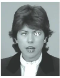
As a real-world test of this classifier, a complete human passport image (Figure 7) has been scanned by the classifier using a scanning window of approximately eye size.
Center pixels which have elicited a positive eye response in their corresponding scanning window are marked in black or white, dependent on the local contrast so as to be best vis-ible.Figure 7shows that the eye regions have been detected robustly, with especially the left eye (right half of the im-age) having a large number of positive identifications. Faulty classifications are reported for the lower lip and part of the collar. This classification could be reached with a two IC hardware-based version of the classifier and LOC operator, with possibly a low-performance microprocessor to do a
final model-based geometric analysis and select the correct eye locations. Thus, the goal of computing high-quality fea-tures and reducing data rate for subsequent high-level pro-cessing stages could easily be achieved in this image anal-ysis/segmentation application. The operator has also been tested in a similar classification testbench with sample im-ages of a production line for circuit breakers. The aim was quality inspection, that is, discerning and discarding faulty breakers. Testing of the LOC operator in this application also brought comparably high-classification results, proving the efficacy of the computed features for a task of quite diff er-ent scope, as well as indicating the broad range of tasks the modified operator could be used on.
Even though the discussed image operator is not a very recent development [7], when compared to state-of-the-art image operators for texture and local orientation analysis [3,6], it can be reasoned that LOC gives qualitatively simi-lar results. As mentioned in the introduction, the aim of this research is not to develop a hardware sensor dedicated (and limited!) to one single application, but one that produces a selection of salient features comprising local image structures in such a way that subsequent software-based processing stages have a greatly reduced work load while still being able to extract high-level image information such as the examples mentioned above. Macroscopic textures/features such as the ones analyzed in [4] are characterized by a distinct local mix-ture of microscopic, that is, LOC texmix-ture feamix-tures. Local his-tograms of the LOC features would thus be sufficient to sep-arate macroscopic textures. Macroscopic image orientation could also be computed from the LOC features, with 8 main directions (in the case of anN8neighborhood LOC) instantly available from the increased local occurrence of single, elon-gated features such as feature 6 ofFigure 2(compare lines in
Figure 3). Intermediate image orientations are characterized
by a mix of the LOC features closest in orientation to the one exhibited by the image, which also makes them discernible in localized histograms. Even if subsequent stages need to oper-ate on the raw image data, they could still use the hardware LOC sensor as a region-of-interest (ROI) selector, choosing to do high-level image analysis only on the regions denoted by LOC features, which indicate relevant image information (Figures3and4).
However, because of accuracy and dynamic range require-ments, the variable current scaling (5) has been implemented in a somewhat modified translinear circuit, using fixed cur-rent multiplication in curcur-rent mirrors and subsequent vari-able current splitting in a differential amplifier [12].
InFigure 8, the circuit for computing an absolute value
current is shown, as adapted from [9]. A biasing current for P1 and P4 is derived from the (reduced) current output flowing through N2, with N1 having about one tenth of the W/L of N2. P1 and P4 in turn bias their counterparts P2 and P5. If a current is drawn from Iin to ground/VSSA, pMOS transistors P2 and P3 act as current mirror, and the voltage node at input Iinis drawn to ground because of the increased VGS of P2 compared to P1 (with its smaller biasing current relative to Iin), thus turning offP5. Current Iinis then simply forwarded through P2 and P3 to N2, where it can be used as a gate voltage VequIoutfor nMOS transistors matched to N2 to distribute Iin. In the second case, that is, a current is flowing into Iin from the supply rail VDDA, the VGS of P5 will in-crease, thus increasing the potential at node Iinand turning of P2, because the gate voltage of P5 is defined (i.e., fixed) by P4. In this case, P5 acts as a current conveyor or pass tran-sistor, forwarding Iinto N2. Hence, irrespective of the direc-tion of the current into Iin (source/sink), it will always flow through N2 in the same direction.
The complete pixel cells consist of the following (com-pare to Figures9and10, which depict the layout and block diagram, resp.):
(i) the photo diode1,
(ii) time-continuous diffusion network 2 for the ad-justable averaging of local light levels (3),
(iii) absolute current value circuit3to compute the ab-solute difference between local average and photo cur-rent of the cell (5),
(iv) the current amplifier4for scaling the absolute dif-ference to achieve different feature sensitivity [12] (5), (v) the current mirrors5to compute the reference com-posed of the difference between photo current and scaled absolute difference ((1), modified witht(m,n) of (5)),
(vi) the current comparators8to compare the reference to the neighbor photo currents (1),
1 2 3 4
9 5 6
7
8
Figure9: Layout of the pixel cell implementation.
(vii) a translinear circuit to normalize the reference with the photo current and compare the normalized result to an external threshold to achieve a measure for the vari-ability in local photo currents6,
(viii) the SRAMs to store the comparison results (9 Bit)7, (ix) digital readout circuitry9,
(x) equation (2) is performed implicitly by reading each single comparison bit off-chip, rather than computing a feature sum in the pixel cell itself.
1
Photocurrent of the pixel cell Photocurrents of 8 surrounding pixels Light sensitivity adjust
Diffusion network (local Gaussian smoothing)
σ-adjustment/smoothing
2
Phot
ocur
re
nt
Iσ
Sm
o
o
th
ed
IP IP
Difference ( )
Δ
I
Absolute value ()
3
Δ
I
ΔI 6
Normalization (/) ΔI/Iσ
Scaling (C
) 4
Scale range select Scaling factor
IS
+
Computation of reference value 5
IRef Continous-time circuit
8
Comparison of photocurrents (surrounding pixels) with reference value Comparison of normalized absolute
difference with external threshold Threshold
Save enable
7
SRAM, 9-Bit latch
Bus control 9
Select X Bus multiplexer Discrete-time circuit
Output pixel cell: 5 digital lines
Figure10: Block diagram of the pixel cell implementation.
well as defining the readout sequence for the tristate digital feature bus.
Figure 11illustrates the temporal performance of a pixel
cell. The photo current for the middle pixel is 20 pA and the output of the current comparators after a stimulus change at the sensor input for three selected neighbors at t=20 ms is shown. The reference value as illustrated inFigure 10(step
5) is 8.3 pA, as computed from the middle pixel photo cur-rent, the output of the resistive network of 11.6 pA, and a scalingCequal to 1. The stimuli change from uniform 0 pA to (from top to bottom) 50, 10, 5 pA.
The computation times (6.8, 14.4, resp., 24.2 ms) are comparable to the ones reported in [6]. However, because of the time-continuous nature of the analog computation in the
pixel cell, the LOC features can be read from the pixel cells at any given time, there is no hardware reset or integration time needed [6], changes to lower-light levels simply take more time to propagate to the LOC feature output. Hence, there is no “frame rate” per second. The frame rate reported in
Table 1has been chosen to represent standard room lighting,
with the lowest light level generating about 50 pA photo cur-rent. The entire analog feature extraction has been simulated over 4 decades of photo current, that is, 1 pA to 10 nA (13 Bit), equivalent to an operability of the sensor and feature extraction ASIC over a range from bright daylight to dark twilight.
computa-20 40 Time (ms)
Figure 11: Response time of pixel cell from input current (i.e., brightness) change to feature output (stimuli change at 20 ms).
Table1: (Simulated) characteristics of the LOC pixel cell/sensor ar-ray.
Technology 1P3M 0.6μm CMOS
Pixel cell size (83×80)μm2=6640μm2
Pixel cell fill factor 3.8% Pixel cell dynamic range 84 dB
Pixel cell absolute accuracy 25 dB (10 pA) 28 dB (10 nA) ASIC size 1560μm×2240μm ASIC frame rate 140 ASIC array size 16×26 pixel cells ASIC power
161μW Consumption (analog)
ASIC power consumption
10μW (digital) (without bonding
capacity, only bondpads)
tions, establishing a 25 dB accuracy at low photo currents of 10 pA, and 28 dB at 10 nA with a confidence of 90%. Two counteracting effects have been observed which act to keep accuracy almost constant over the whole dynamic range. On the one hand, translinear circuits work best at low-current levels, where all transistors are operating firmly in subthresh-old [10], on the other hand, current mirrors, which are em-ployed in various stages of the analog computation, are sub-ject to statistical variations at low currents, improving pro-gressively with higher current levels [9].
fication discussed in Section 2.2still gives 100% classifica-tion result with “decaying exponential” smoothing. Third, the accuracy numbers obtained from the Monte-Carlo sim-ulation have been used in the form of an artificially in-troduced 5% (∼= 26 dB) error (uniform distribution) on the right-hand side of (1), that is,b(n,m)−t(n,m). While this represents a rather crude approximation of the Monte-Carlo outcomes, it also reflects an upper bound, since the real error is more centered around a mean. Incorporating this error in the EE/ENE classification results in one er-roneous classification of an eye sample (EE class) as ENE class.
The pixel cell has been realized with a size of (83×
80)μm2. The corresponding ASIC with additional analog and digital interface and control circuitry has been manu-factured, but measurement results are not yet available. It is operating in a simple scan mode, with all LOC feature latches connected to the same bus via tristate gates. The digital power consumption given inTable 1reflects the power con-sumed by the latches when charging bus and bondpad capac-ity, as well as the power consumed by the pixel address coun-ters and decoders, and address lines, at the indicated frame rate. Simulated performance characteristics for the pixel cell are given inTable 1.
2.4. Future developments
Current research work deviates from the continuous time analog implementation described herein. While the opera-tor is quite successful and comparably easy to implement in hardware in the modified fashion, still simpler variants of it could be explored. An especially promising avenue of explo-ration is the field of pulse-based image processing. Given a pulsing pixel cell as an input, whose pulse rate is equivalent to the grayscale value of the pixel, it has been found that a simple rank order coding theorized from biological evi-dence of pulse computation is capable of producing very sim-ilar features to the ones discussed herein [13]. This rank or-der coding can be achieved using digital variants of synapses and neurons. Error-prone analog normalization, scaling, ad-dition, and subtraction can all be eliminated from the pixel cell, resulting in a predominantly digital and more robust im-plementation, as well as reducing the design time. Also, the output signal can be easily represented in a pulse form and fed to, for example, a pulse-based clustering algorithm, or be used for various digital processing stages, since pulse com-putations of this nature are very similar to digital informa-tion representainforma-tions. In contrast to the conveninforma-tional digital image filtering discussed in [1], this processing would still be fully parallel and can be incorporated into the pixel cell in the same manner as the analog computation discussed herein.
3. CONCLUSION
We have presented a scheme for fast, computationally inex-pensive, massively parallel and flexible hardware-based fea-ture extraction. Quality of the feafea-ture extraction has been documented using a sample eye finder application as well as sample images from an early feasibility study of a car overtake monitoring system. In both cases, highly significant points of the ROI have been extracted and their efficacy in distin-guishing target shapes, that is, eyes, is shown. The original image operator has been adjusted with respect to connec-tivity, parameters, and computational requirements for the ease of the analog/mixed-signal hardware implementation. An HDR CMOS sensor design has been carried out to take full advantage of the analog dynamic ranges and computa-tional domains possible on a modern CMOS process while still achieving a digitally coded, data rate reduced feature out-put. This feature output can be used on-chip, that is, with a digital histogram computation over a selected ROI, to extract a feature vector for that ROI which can be fed directly into a classifier network or be used for further computations off -chip.
ACKNOWLEDGMENTS
The major part of the reported work has been carried out in the Projects GAME and GAMPAI which were funded in the research program VIVA SPP 1076 by the German re-search foundation “Deutsche Forschungsgemeinschaft.” All responsibility for this paper is with the authors. The au-thors thank Austria Mikro Systeme International AG for the
technical support and the D4D group, TU Dresden, com-puter science, AI Institute, for the kind providance of project-related data and information. The contributions of Michael Eberhardt, Robert Wenzel, Jens D¨oge, and Jan Skribanowitz to the project in general and their invaluable technical as-sistance to the presented work are gratefully acknowledged. Many thanks also go to the three anonymous reviewers for their helpful comments on improving the quality and clarity of this paper.
REFERENCES
[1] B. Tongprasit, K. Ito, and T. Shibata, “A computational digital-pixel-sensor VLSI featuring block-readout architecture for pixel-parallel rank-order filtering,” inProceedings of the IEEE International Symposium on Circuits and Systems (ISCAS ’05), vol. 3, pp. 2389–2392, Kobe, Japan, May 2005.
[2] A. Elouardi, S. Bouaziz, A. Dupret, J. O. Klein, and R. Reynaud, “Image processing vision system implementing a smart sen-sor,” inProceedings of the 21st IEEE Instrumentation and Mea-surement Technology Conference (IMTC ’04), vol. 1, pp. 445– 450, Como, Italy, May 2004.
[3] N. Massari, M. Gottardi, L. Gonzo, D. Stoppa, and A. Simoni, “A CMOS image sensor with programmable pixel-level ana-log processing,”IEEE Transactions on Neural Networks, vol. 16, no. 6, pp. 1673–1684, 2005.
[4] B. Zitov´a, J. Kautsky, G. Peters, and J. Flusser, “Robust de-tection of significant points in multiframe images1,”Pattern Recognition Letters, vol. 20, no. 2, pp. 199–206, 1999.
[5] A. K¨onig, C. Mayr, T. Bormann, and C. Klug, “Dedicated implementation of embedded vision systems employing low-power massively parallel feature computation,” inProceedings of the 3rd VIVA-Workshop on Low-Power Information Process-ing, pp. 1–8, Chemnitz, Germany, March 2002.
[6] P.-F. R¨uedi, P. Heim, F. Kaess, et al., “A 128×128 pixel 120-dB dynamic-range vision-sensor chip for image contrast and orientation extraction,” IEEE Journal of Solid-State Circuits, vol. 38, no. 12, pp. 2325–2333, 2003.
[7] C. Goerick and M. Brauckmann, “Local orientation coding and neural network classifiers with an application to real time car detection and tracking,” inProceedings of the 16th Sympo-sium of the DAGM and the 18th Workshop of the ¨OAGM, W. Kropatsch and H. Bischof, Eds., Springer, New York, NY, USA, 1994.
[8] A. K¨onig, M. Eberhardt, and R. Wenzel, “A transparent and flexible development environment for rapid design of cog-nitive systems,” inProceedings of 24th Euromicro Conference, vol. 2, pp. 655–662, Vasteras, Sweden, August 1998.
[9] A. G¨unther, “Design of a library of scalable, low-power CMOS cells for classification and feature extraction in integrated cog-nition systems,” Diploma thesis, University of Technology, Dresden, Germany, April 2000.
[10] B. A. Minch, “Analysis and synthesis of static translinear cir-cuits,” Tech. Rep. CSL-TR-2000-1002, Computer Systems Lab-oratory, Cornell University, Ithaca, NY, USA, 2000.
[11] L. Raffo, “Analysis and synthesis of resistive networks for dis-tributed visual elaborations,”Electronics Letters, vol. 32, no. 8, pp. 743–744, 1996.
ests include optimization tools such as genetic algorithms, immune systems on-chip, bioinspired circuits in general, information pro-cessing in spiking neural nets in both simulation and hardware, and mixed-signal VLSI design, for example, pixel sensors and CMOS subthreshold circuits. He is the author or coauthor of 14 publica-tions in the subject areas mentioned above and has acted as a re-viewer for NIPS conferences.
Andreas K¨onigstudied electrical engineer-ing, computer architecture, and VLSI de-sign at Darmstadt University of Technol-ogy and obtained the Ph.D. degree in 1995 from the same university, Institute of Mi-croelectronic Systems, in the field of neural network application and implementation. In 1995, he joined Fraunhofer-Institute IITB for research on visual inspection and aerial/satellite image processing. In 1996, he