Volume 2007, Article ID 45605,16pages doi:10.1155/2007/45605
Research Article
Second-Order Optimal Array Receivers for
Synchronization of BPSK, MSK, and GMSK
Signals Corrupted by Noncircular Interferences
Pascal Chevalier, Franc¸ois Pipon, and Franc¸ois Delaveau
Thales-Communications, EDS/SPM, 160 Bd Valmy, 92704 Colombes Cedex, France
Received 4 October 2006; Revised 16 March 2007; Accepted 13 May 2007
Recommended by Benoit Champagne
The synchronization and/or time acquisition problem in the presence of interferences has been strongly studied these last two decades, mainly to mitigate the multiple access interferences from other users in DS/CDMA systems. Among the available re-ceivers, only some scarce receivers may also be used in other contexts such as F/TDMA systems. However, these receivers assume implicitly or explicitly circular (or proper) interferences and become suboptimal for noncircular (or improper) interferences. Such interferences are characteristic in particular of radio communication networks using either rectilinear (or monodimensional) modulations such as BPSK modulation or modulation becoming quasirectilinear after a preprocessing such as MSK, GMSK, or OQAM modulations. For this reason, the purpose of this paper is to introduce and to analyze the performance of second-order optimal array receivers for synchronization and/or time acquisition of BPSK, MSK, and GMSK signals corrupted by noncircular interferences. For given performances and in the presence of rectilinear signal and interferences, the proposed receiver allows a reduction of the number of sensors by a factor at least equal to two.
Copyright © 2007 Pascal Chevalier et al. This is an open access article distributed under the Creative Commons Attribution License, which permits unrestricted use, distribution, and reproduction in any medium, provided the original work is properly cited.
1. INTRODUCTION
The synchronization and/or time acquisition problem in the presence of interferences has been strongly studied these last two decades, mainly to mitigate the multiple access interfer-ences (MAI) from other users in DS/CDMA systems. The available receivers may be implemented from either mono-antenna [1–7] or multi-antennas [8–12]. Receivers presented in [9,12] are analog receivers while the other ones are digi-tal receivers. Most of the available digidigi-tal receivers are very specific of the CDMA context and cannot be used elsewhere, since they require assumptions such as a spreading sequence which is repeated at each symbol [1–7], a very large number of MAI [11], no data on the codes [8,11] or periodic and or-thogonal sequences [8]. On the other hand, [5], which does not require the previous assumptions, assumes interferences with known delays and spreading sequences, which corre-sponds to very specific situations. On the contrary, although assuming orthogonal and periodic codes, maximum likeli-hood (ML) receivers presented in [10] belong to the family of the scarce receivers which may be used in other contexts than DS/CDMA systems such as F/TDMA systems in
analyze the performance of the SO optimal array receiver for synchronization and/or time acquisition of BPSK signals cor-rupted by noncircular, and more precisely by rectilinear in-terferences. This receiver, patented recently [20], implements an optimal, in an LS sense, widely linear (WL) [21] spatial filtering of the data followed by a correlation operation with a training sequence. Extensions of these results to MSK and GMSK signals [16] are presented at the end of the paper and constitute the second purpose of this paper.
The first use of WL filters in signal processing has been reported in [22], the first discussion about their interest for cyclostationary signals has been introduced in [23,24] and the proof of their optimality in SO noncircular context has been presented in [21,25,26]. Since the previous papers, op-timal WL filtering has raised an increasing interest this last decade in radio communications for demodulation purposes (see [17] and references therein). However, up to now and to our knowledge, despite some works about frequency-offset estimation in noncircular contexts [27–29], optimal WL fil-tering has never been investigated for synchronization and/or time acquisition purposes in noncircular contexts, hence the present paper. Note that some results of the paper have al-ready been partially presented in the conference paper [30].
After an introduction of some notations, hypotheses, and data statistics in Section 2, the SO optimal array receiver for synchronization and/or time acquisition of a BPSK sig-nal corrupted by noncircular interferences is presented in Section 3, where some general interpretations, properties, and performance of this receiver are described. Some insigths into the performance of the latter in the presence of one recti-linear interference are presented and illustrated inSection 4. Section 5 investigates extensions of the previous results to MSK and GMSK signals. FinallySection 6concludes the pa-per.
2. HYPOTHESES AND PROBLEM FORMULATION FOR BPSK SIGNALS
2.1. Hypotheses
We consider an array ofNnarrowband (NB) sensors receiv-ing the contribution of a BPSK signal and a total noise com-posed of some potentially SO noncircular interferences and a background noise. This situation is, for example, character-istic of a BPSK radio communication network where inter-ferences correspond to cochannel interinter-ferences (CCI) gener-ated by the network itself. The complex envelope of the useful BPSK signal is, to within a constant, given by
s(t)=
n
anv(t−nT), (1)
wherean = ±1 is the transmitted symboln,T is the
sym-bol duration, and v(t) is a real-valued pulse-shaped filter such that rv(t) v(t)⊗v(−t)∗ is a Nyquist filter, that is,
rv(nT) = 0 forn /= 0. Symbols⊗and∗are the
convolu-tion and the complex conjugaconvolu-tion operaconvolu-tions, respectively. Note that rv(t) is the autocorrelation of v(t) and the
pre-vious condition is verified if v(t) is either a raised cosine pulse-shaped filter or a rectangular pulse of durationT. In
most of radio communication systems,K training symbols an (0 ≤ n ≤ K −1) are periodically transmitted among
information symbols for synchronization and/or time ac-quisition purposes. TheseKtraining symbols are known by the receiver and can be considered as deterministic symbols. On the contrary, the information symbols are unknown by the receiver, are random and can be considered as i.i.d sta-tionary symbols. For example, in a burst transmission, one training sequence ofK symbols jointly with some informa-tion symbols are transmitted at each burst. Assuming a use-ful propagation channel withMmultipaths, notingx(t) the vector of the complex envelopes of the signals at the out-put of the sensors, Te the sample period such thatT/Te is
an integerq,sv(kTe) s(t)⊗v(−t)∗/t=kTe andxv(kTe)
x(t)⊗v(−t)∗/t=kTethe sampled useful signal and observation
vector at the output of the matched filterv(−t)∗, we obtain
xv
kTe
≈
M−1
i=0
μssv
kTe−τi
hsi+bTv
kTe
. (2)
In this equation,μsis a real parameter controlling the
trans-mitted amplitude of the useful signal,τiandhsiare the delay
and the channel vector of the useful pathi,bTv(kTe) is the
sampled total noise vector at the output of v(−t)∗, which contains the contribution of interferences and background noise and which is assumed to be uncorrelated with all the signalssv(kTe−τi). In a digital radio communication system,
the synchronization function aims at detecting the diff er-ent useful paths (interception) and estimating their delaysτi
(time acquisition). For equalization/demodulation purposes, it aims also at choosing the best sampling time, from the es-timated power of each detected path, and at optimally po-sitioning the equalizer with respect to the delays of the tected paths. The synchronization process is thus a joint de-tection and estimation problem. Of course, the probability to improve the best sampling time increases with the degree of data oversampling. In such a context, there is no need to exactly estimate the delaysτi(0≤i≤M−1) and the
prob-lem rather consists, for each useful pathi0, to detect the most
powerful sample associated with this path. More precisely, for each useful pathi0, noting loTe the sample time which
is the nearest ofτi0, the problem considered in this paper is
both to detect the presence of the useful pathi0and to find
the best estimate ofloTe from the sampled observation
vec-tors. Assuming an optimal sampling time for the pathi0, the
sampled observation vector considered in practice can then be written as
xv
kTe
≈μssv
k−lo
Te
hs+bTv
kTe
. (3)
In this equation,hsis the channel vector of the useful path
i0andbTv(kTe)is the sampled contribution of both the
to-tal noise vectorbTv(kTe) and the useful paths different from
i0. Note thatbTv(kTe) =bTv(kTe) for a useful propagation
assumes that the carrier frequency of the useful signal is a pri-ori known (which is true for cellular networks) or has been perfectly compensated.
2.2. Second-order statistics of the data
The SO statistics of the data considered in the follow-ing correspond to the first and second correlation matrix of xv(kTe), defined by Rx(kTe) E[xv(kTe) xv(kTe)†]
andCx(kTe) E[xv(kTe) xv(kTe)T], respectively, where T
and † correspond to the transposition and transposi-tion conjugatransposi-tion operatransposi-tion respectively. In a same way, the first and second correlation matrix of bTv(kTe)
are defined by R(kTe) E[bTv(kTe) bTv(kTe)†] and
C(kTe) E[bTv(kTe) bTv(kTe)T], respectively. The first
and second correlation matrix of bTv(kTe) are defined
by R(kTe) E[bTv(kTe) bTv(kTe)†] and C(kTe)
E[bTv(kTe) bTv(kTe)T] respectively. Note thatR(kTe) =
R(kTe) andC(kTe)=C(kTe) for a useful propagation
chan-nel with no delay spread. Note also thatC(kTe)=O(resp.,
C(kTe) = O) for allk for an SO circular vectorbTv(kTe)
(resp.,bTv(kTe)), whereOis the (N×N) zero matrix. Finally
we noteπs(kTe)E[|sv(kTe)|2] the instantaneous power of
the transmitted useful signal forμs=1. Note that the
previ-ous statistics depend on the time parameter since the consid-ered useful signal and interferences are cyclostationary, due to their digital nature.
2.3. Problem formulation
Since theK training symbolsan(0 ≤ n ≤ K −1), which
are periodically transmitted for synchronization purposes, are known by the receiver, the associated useful samples sv(nT) = rv(0)an(0 ≤ n ≤ K−1) are also known by the
receiver. Then, a first way to solve the synchronization prob-lem consists to find, for each useful pathi0, the best estimate,
lo, oflo. This can be done by searching for the integerslfor
which the known useful samplessv(nT) (0 ≤ n ≤ K−1)
are optimally estimated, in an LS sense, from the observation vectorsxv((l/q+n)T), 0≤n≤K−1. We solve this
prob-lem in Section 3.1, without any assumptions about the de-lay spread of the propagation channels, the orthogonality or the periodicity of the training sequence, contrary to [8,10]. A second way to solve the synchronization problem consists to optimally detect each useful pathi0. This can be done by
searching for the integerslfor which the known useful sam-plessv(nT) (0≤n≤K−1) are optimally detected from the
observation vectorsxv((l/q+n)T), 0≤n≤K−1. We solve
this problem inSection 3.2under particular theoretical as-sumptions, showing offthe hypotheses under which the two ways to solve the synchronization problem are equivalent to each other.
3. OPTIMAL SYNCHRONIZATION FOR BPSK SIGNALS
It is now well known [17,21,25,26] that the linear filters are SO optimal for SO circular observations only but be-come sub-optimal in noncircular contexts for which the SO
optimal filters are WL, weighting linearly and independently the observations and their complex conjugate. In these con-ditions, the first way to solve, in the presence of noncircu-lar interferences, the synchronization problem presented in Section 2.3is, for each useful pathi0, to search for the
opti-mal integerl, notedlo, for which the known useful samples,
sv(nT)=rv(0)an(0≤n≤K−1), are optimally estimated,
in an LS sense, from a WL spatial filtering of the observation vectorsxv((l/q+n)T) (0 ≤ n ≤ K−1). This gives rise in
Section 3.1to the optimal LS array receiver, called OPT-LS receiver, for synchronization of the BPSK useful signal in the presence of noncircular interferences. This OPT-LS receiver is shown inSection 3.2to also correspond, under some the-oretical assumptions not required in practice, to the array receiver for whichloallows the optimal detection, in terms
of the generalized likelihood ratio test (GLRT) [31], of the known useful samples,sv(nT) (0 ≤ n ≤ K−1), from the
observation vectorsxv((lo/q+n)T) (0≤n≤K−1). An
en-lightening interpretation and some performance of the OPT-LS receiver are then presented in Sections3.3and3.4, respec-tively. Note that the results presented in this section are com-pletely new.
3.1. Presentation of the OPT-LS receiver
Synchronization or time acquisition from OPT-LS receiver consists to find, for each useful pathi0, the integerl, noted
lo, which minimizes the LS error,εWL(lTe,K), between the
known samplessv(nT)=rv(0)an(0≤n≤K−1) and their
LS estimation from a WL spatial filtering of the dataxv((l/q+
n)T) (0≤n≤K−1). The LS error,εWL(lTe,K), is defined
by
εWL
lTe,K
1
K
K−1
n=0
sv(nT)−w
lTe
†
xv
l
q+n T
2
,
(4)
wherexv((l/q+n)T)[xv((l/q+n)T)T,xv((l/q+n)T)†]T
and wherew( lTe) [w1(lTe)T,w2(lTe)T]Tis the (2N×1)
WL spatial filter which minimizes the criterion (4). This filter is defined by
wlTe
=w1
lTe
T
,w1
lTe
†T =Rx
lTe
−1
rxs
lTe
,
(5)
where the vectorrxs(lTe) and the matrixRx(lTe) are given by
rxs
lTe
1
K
K−1
n=0
xv
l
q+n T sv(nT)
∗, (6)
Rx
lTe
1
K
K−1
n=0
xv
l
q +n T xv
l q+n T
†
. (7)
Using (5) to (7) into (4), we obtain a new expression of
εWL(lTe,K) given by
εWL
lTe,K
=
1 K
K−1
n=0
sv(nT)2
1−COPT-LS
lTe,K
=πs
1−COPT-LS
lTe,K
,
where πsr(0)2 is the input power of the useful BPSK
samples,sv(nT), andCOPT-LS(lTe,K) such that 0≤COPT-LS×
(lTe,K)≤1 is given by
COPT-LS
lTe,K
1
πs rxs
lTe
†
Rx
lTe
−1
rxs
lTe
. (9)
We deduce from (8) that for each useful pathi0, the
parame-terlolocally maximizes the sufficient statisticCOPT-LS(lTe,K)
given by (9). As a consequence, the estimated sampled de-lays of all the useful paths correspond to the sample timeslTe
for whichCOPT-LS(lTe,K) is locally maximum. If the number,
M, of useful paths is a priori known, their estimated sam-pled delays correspond to the positions of the M maxima of COPT-LS(lTe,K). However, if M is not known a priori, a
threshold has to be introduced to limit the false alarm rate (FAR). In these conditions, the estimated sampled delays of the useful paths correspond to the sample timeslTefor which
COPT-LS(lTe,K) is locally maximum and above the threshold.
The approach considered in thisSection 3.1does not require any assumption about the propagation channels, the interfer-ences and the training sequence. Thus, in practice, OPT-LS receiver may be used for synchronization or time acquisition in the presence of arbitrary propagation channels and inter-ferences. Note that the receiver presented in [8] for the same problem, called conventional LS array receiver and noted CONV-LS receiver in the following, is deduced from a sim-ilar LS approach but takes into account only a linear spatial filtering of the data,xv((l/q+n)T) (0≤n≤K−1), instead of
a WL one. It gives rise to the conventional sufficient statistic
CCONV-LS(lTe,K) such that 0≤CCONV-LS(lTe,K)≤1, defined
by
CCONV-LS
lTe,K
1
πs
rxs
lTe
†
Rx
lTe
−1
rxs
lTe
,
(10)
where the vectorrxs(lTe) and the matrixRx(lTe) are defined
by (6) and (7), respectively but where the vectorxv((l/q+
n)T) is replaced byxv((l/q+n)T). This conventional receiver
is the heart of the interference analyzer described in [32] for the GSM network monitoring.
3.2. Interpretation of OPT-LS and CONV-LS receivers in terms of GLRT-based detectors 3.2.1. Theoretical assumptions
In this section, we present the assumptions under which OPT-LS and CONV-LS receivers forl = loalso correspond
to the GLRT-based receiver for the detection of the known samples sv(nT) = rv(0)an (0 ≤ n ≤ K −1) from the
observation vectors xv((lo/q +n)T) (0 ≤ n ≤ K −1).
Note that these assumptions are theoretical, are not neces-sarily verified in practical situations and are absolutely not required in practice to successfully implement the conven-tional and optimal receivers defined by (10) and (9), respec-tively. However, these assumptions allow in particular to get more insights into the situations for which (9) and (10) be-come optimal from a GLRT-based detection point of view. Besides, they allow to show off the optimality of (9) and (10) in the presence of SO noncircular and circular total
noise, respectively. Defining the vector bTv((l/q+n)T) by
bTv((l/q+n)T)[bTv((l/q+n)T)T,bTv((l/q+n)T)†]T, these
theoretical assumptions correspond to the following.
(A1) The samplesbTv((lo/q+n)T), 0≤n≤K−1 are
un-correlated to each other.
(A2) The matricesR((lo/q+n)T) andC((lo/q+n)T) do not
depend on the symbol indicen.
(A3) The matricesR((lo/q+n)T),C((lo/q+n)T) and the
vectorhsare unknown.
(A4) The samplesbTv((lo/q+n)T), 0 ≤ n ≤ K −1, are
Gaussian.
(A5) The samplesbTv((lo/q+n)T), 0≤n≤K−1, are SO
noncircular.
(A6) The samplesbTv((lo/q+n)T) andsv(mT), 0≤n,m≤
K−1, are statistically independent.
(A7) The useful propagation channel has no delay spread (bTv((lo/q+n)T)=bTv((lo/q+n)T)).
Note that contrary to [8,10], no assumption is made about the correlation properties of the training sequence. (A1) would only be true for interference propagation channels with no delay spread as soon as the rectilinear interferences would be generated by the network itself (internal BPSK in-terferences) and would be synchronous with the useful signal to verify the Nyquist criterion. (A2) would be true for cyclo-stationary interferences with symbol periodT, as it would be the case for internal BPSK interferences. (A4) could not be verified in the presence of rectilinear interferences and would be a false assumption allowing to only exploit the SO statis-tics of the observations from a GLRT approach. (A5) would be true in the presence of rectilinear interferences in particu-lar but is generally not exploited in detection problems. (A6) would always be verified due to the deterministic character ofsv(mT) (0≤m≤K−1) jointly with the zero-mean and
random character of the total noise. Finally, (A7) would be valid for some particular applications.
3.2.2. GLRT-based receiver for detection
To compute the GLRT-based receiver for detection, we con-sider the optimal delayloTeand the detection problem with
two hypotheses H0 and H1, where H0 and H1 correspond to the presence of total noise only and signal plus total noise into the observation vectorxv((lo/q+n)T), respectively.
Un-der these two hypotheses, using (2), (3), and (A7), the vector xv((lo/q+n)T) can be written as
H1 : xv
lo
q +n T ≈μssv(nT)hs+bTv
lo
q +n T , (11a)
H0 : xv
lo
q +n T ≈bTv
lo
q +n T . (11b)
According to the Neyman-Pearson theory of detection [31] and using (A6), the optimal receiver for detection of sam-plessv(nT) fromxv((lo/q+n)T) over the training sequence
to compare to a threshold the function LR(loTe,K) defined
by
LRloTe,K
p
xv
lo/q+n
T, 0≤n≤K−1,/H1 pxv
lo/q+n
T, 0≤n≤K−1,/H0. (12)
In (12), p[xv((lo/q+n)T), 0 ≤ n ≤ K−1,/Hi] (i = 0, 1)
is the conditional probability density of [xv(loTe),xv(loTe+
T),. . .,xv(loTe+ (K−1)T)]Tunder Hi. Using (11) into (12),
and recalling thatsv(nT) is a deterministic quantity, we get
LRloTe,K
p[A]
p[B], (13)
(whereA= {bTv((lo/q+n)T)=xv((lo/q+n)T)−μssv(nT)hs,
0≤n≤K−1}, andB= {bTv((lo/q+n)T)=xv((lo/q+n)T),
0≤n≤K−1}).
Using (A1), (A2), and (A4), expression (13) takes the form
LRloTe,K
=
K−1
n=0p[Sn]
K−1
n=0p[Dn]
, (14)
(Sn={bTv((lo/q+n)T)=xv((lo/q+n)T)−μssv(nT)hs/sv(nT),
μshs,R(loTe),C(loTe)},Dn = {bTv((lo/q+n)T)=xv((lo/q+
n)T)/R(loTe),C(loTe)}).
From (A2), (A4), and (A5), the probability density of bTv((lo/q+n)T) becomes a function ofbTv((lo/q+n)T) given
by [33,34]
p
bTv
lo
q +n T π−NdetRb
loTe
−1/2
×exp
−
1 2 bTv
lo
q +n T
†
×Rb
loTe
−1
bTv
lo
q +n T . (15)
Using (15) into (14), we obtain
LRloTe,K
=
K−1
n=0p[En]
K−1
n=0 p[Fn]
, (16)
(En={bTv((lo/q+n)T)=xv((lo/q+n)T)−μssv(nT)hs/sv(nT),
μshs,Rb(loTe)},Fn = {bTv((lo/q+n)T) =xv((lo/q+n)T)/
Rb(loTe)}), andhs[hsT,hs†]Tand whereRb(loTe) is defined
by
Rb
loTe
E
bTv
lo
q +n T bTv
lo
q +n T
†
=
⎛ ⎝R
loTe
CloTe
CloTe
∗
RloTe
∗
⎞ ⎠.
(17)
Note that matrix Rb(loTe) contains the information about
the potential noncircularity of the total noise through the matrix C(loTe), which is not zero for SO noncircular total
noise. As, from (A3), μshs andRb(loTe) are assumed to be
unknown, they have to be replaced in (16) by their maxi-mum likelihood (ML) estimates, giving rise to a GLRT ap-proach. In these conditions, it is shown in the appendix that a sufficient statistic for the optimal detection, from a GLRT point of view, ofsv(nT) (0 ≤ n ≤K −1) from the
obser-vation vectorsxv((lo/q+n)T) (0 ≤ n ≤ K−1), is, under
the assumptions (A1) to (A7), given byCOPT-LS(loTe,K)
de-fined by (9). We deduce from the previous results that, under the theoretical assumptions (A1) to (A7), not necessarily ver-ified and not required in practice, the optimal synchroniza-tion and time acquisisynchroniza-tion of the useful BPSK signal from the GLRT approach consists to compute, for each sample time lTe, the quantityCOPT-LS(lTe,K), defined by (9), and to
com-pare it to a threshold. The sampled delays of the useful paths thus correspond to the sample timeslTewhich generate
lo-cal maximum values ofCOPT-LS(lTe,K) among those which
are over the threshold. Thus theoretical assumptions (A1) to (A7) allow to give conditions of optimality of the OPT-LS receiver, in the GLRT sense, among which we find the condition of SO noncircularity of the total noise, valid for rectilinear interferences in particular. Nevertheless, when at least one of the assumptions (A1) to (A7) is not verified, as it may be the case for most practical situations, receiver (9) is no longer optimal in terms of detection but this does not mean that it does not work in practice. Note finally that a similar GLRT approach, but made under the theoretical as-sumptions (A1bis), (A2), (A3), (A4), (A5bis), (A6) and (A7), where (A1bis) and (A5bis) are defined by
(A1bis) the samplesbTv((lo/q+n)T), 0 ≤ n ≤ K−1, are
uncorrelated to each other,
(A5bis) the samplesbTv((lo/q+n)T), 0≤n≤K−1, are SO
circular,
is reported in [10] and gives rise to the sufficient statistic
CCONV-LS(loTe,K) defined by (10). This shows that (10) is
di-rectly related to a (false) circular total noise assumption and becomes sub-optimal for noncircular total noise.
3.3. Enlightening interpretation
Using (5) into (9) and the fact thatsv(nT) = sv(nT)∗ for
BPSK useful signals, it is easy to verify that, whatever the propagation channel is, the statisticCOPT-LS(lTe,K) defined
by (9), which is a real quantity, takes the form
COPT-LS
lTe,K
=
1 Kπs
K−1
n=0
yvWL
l
q +n T sv(nT), (18)
where yvWL((l/q + n)T) w( lTe)†xv((l/q + n)T) =
2 Re[w1(lTe)†xv((l/q+n)T)] is also a real quantity.
Expres-sion (18) shows that the sufficient statistic COPT-LS(lTe,K)
the output,yvWL((l/q+n)T), of the WL spatial filterw( lTe)
(5) as it is illustrated inFigure 1.
The filterw( lTe) is an estimate of the WL filterw( lTe)
which minimizes the time-averaged mean square error (MSE), εWL(lTe,w), over K observation samples, between
sv(nT) and the real output w†xv((l/q + n)T) = 2 Re×
[w†xv((l/q+n)T)], defined by
εWL
lTe,w
1
K
K−1
n=0
Esv(nT)−w†xv
l
q+n T
2
,
(19)
where w [wT,w†]T. The filter w( lT
e) is thus defined
byw( lTe)Rx,av(lTe)−1rxs,av(lTe)=[w1(lTe)T,w1(lTe)†]T,
whererxs,av(lTe) andRx,av(lTe) are defined by
rxs,av
lTe
1
K
K−1
n=0
E xv l
q +n T sv(nT)
∗, (20)
Rx,av
lTe
1
K
K−1
n=0
E xv l
q +n T xv
l q+n T
†
.
(21)
As a consequence,COPT-LS(lTe,K) is, to within a
normaliza-tion factor, an estimate of the expected value of the correla-tion between the training samplessv(nT) and the outputs of
w(lTe), defined by
COPT-LS
lTe,K
=
1 Kπs
K−1
n=0
E
wlTe
† xv
l
q +n T sv(nT)
= rxs,av
lTe
†
Rx,av
lTe
−1
rxs,av
lTe
πs .
(22)
Considering the detection or time acquisition of the useful path i0, as long as bTv((l/q+n)T) (in (3)) remains
un-correlated withsv(nT), which is in particular the case for a
useful propagation channel with no delay spread, the vector rxs,av(lTe) can be written as
rxs,av
lTe
= 1
K
K−1
n=0
μsE
sv
l−lo
Te
+nTsv(nT)∗hs.
(23)
This vector is collinear tohsand its norm is a function of
(l−lo). In this context, as long as l remains far from lo,
rxs,av(lTe), and thusw( lTe), remain close to zero, which
gen-erates values ofCOPT-LS(lTe,K), and thus ofCOPT-LS(lTe,K),
also close to zero to within the estimation noise due to the finite length of the training sequence for the latter. Aslgets close tolo, the norm ofrxs,av(lTe), and thusCOPT-LS(lTe,K),
increases and reaches its maximum value forl =lo. In this
case, the useful part of the observation vectorxv((lo/q+n)T)
and the training sequencesv(nT) are in phase and the filter
w(loTe) corresponds to the WL spatial matched filter (SMF)
introduced in [17] and defined by
wloTe
=Rx,av
loTe
−1
rxs,av
loTe
=Rb,av
loTe
+μs2πshsh†s
−1
rxs,av
loTe
=w1
loTe
T
,w1
loTe
†T
=
μsπs
1 +μs2πsh†sRb,av
loTe
−1
hs
Rb,av
loTe
−1
hs.
(24)
In (24),Rb,av(loTe)is defined by (21) withbv((lo/q+n)T)
instead of xv((l/q+ n)T). The WL SMF is the WL
spa-tial filter which maximizes the output signal-to-interference-plus-noise ratio (SINR) [17]. Using the previous results, COPT-LS(loTe), defined by (22) withl=lo, takes the form
COPT-LS
loTe
= SINRy[OPT-LS]
1 + SINRy[OPT-LS]=μs
wloTe
† hs.
(25)
In (25), SINRy[OPT-LS] is the SINR at the output of the WL
SMF,w( loTe), defined by the ratio between the time-averaged
powers, over the training sequence duration, of the consid-ered useful pathi0and of the total noise plus other paths at
the output ofw( loTe). This SINR can be written as
SINRy[OPT-LS]=μs2πsh†sRb,av
loTe
−1
hs. (26)
A similar reasoning can be done for the CONV-LS receiver by replacing xv((l/q +n)T) and the WL filter w( lTe) by
xv((l/q+n)T) and the linear filterw( lTe)=Rx(lTe)−1rxs(lTe),
respectively. Structure of CONV-LS receiver is then depicted atFigure 2whereyvL((l/q+n)T)w( lTe)†xv((l/q+n)T),
which is a complex quantity, replacesyvWL((l/q+n)T)
ap-pearing inFigure 1. Forl=loand as long asbTv((l/q+n)T)
remains uncorrelated withsv(nT),w( lTe) becomes an
esti-mate of the well-known linear SMF,w(loTe), defined by
wloTe
Rx,av
loTe
−1
rxs,av
loTe
=Rav
loTe
+μs2πshshs†]−1rxs,av
loTe
=
μsπs
1+μs2πshs†Rav
loTe
−1 hs Rav loTe
−1
hs.
(27)
In (27), Rx,av(loTe) and Rav(loTe) are defined by (21)
with xv((lo/q + n)T) and bv((lo/q + n)T) instead of
xv((l/q+ n)T), respectively, whereas rxs,av(loTe) is defined
by (20) with xv((lo/q + n)T) instead of xv((l/q + n)T).
xv((l/q+n)T)
w(lTe)
yvWL((l/q+n)T)
COPT-LS(lTe,K) ≷βo
sv(nT)
w(lTe)=
Rx(lTe)−1rxs(lTe)
Figure1: Functional scheme of the OPT-LS receiver.
xv((l/q+n)T) w(lTe)
yvL((l/q+n)T)
CCONV-LS(lTe,K) ≷βc
sv(nT)
w(lTe)=
Rx(lTe)−1rxs(lTe)
Figure2: Functional scheme of the CONV-LS receiver.
andCCONV-LS(loTe), defined by (22) withw(loTe) instead of
w(lTe), takes the form
CCONV-LS
loTe
=rxs,av
loTe
†
Rx,av
loTe
−1
rxs,av
loTe
πs
= SINRy[CONV-LS]
1 + SINRy[CONV-LS] =μs
wloTe
† hs.
(28)
In (28), SINRy[CONV-LS] is the SINR at the output of the
SMF,w(loTe), given by [17]
SINRy[CONV-LS]=μs2πshs†Rav
loTe
−1
hs. (29)
Expressions (25) and (28) show that COPT-LS(loTe) and
CCONV-LS(loTe) are increasing functions of SINRy[OPT-LS]
and SINRy[CONV-LS], respectively, approaching unity for
high values of the latter quantities. Note that for a circu-lar total noise, SINRy[OPT-LS] = 2SINRy[CONV-LS]. In
the presence of rectilinear interferences, the WL SMF (24) is shown in [17] to correspond to a classical SMF but for a virtual array of 2N sensors with phase diversity in addi-tion to space, angular, and/or polarizaaddi-tion diversities of the true array ofNsensors. The SMF (27) discriminates the use-ful signal and interferences by the direction of arrival (DOA) and/or polarization (ifN >1) and is able to reject up toN−1 interferences from an array ofNsensors. The WL SMF (24) discriminates the sources by DOA, polarization (ifN > 1) and phase, and is thus able to reject up to 2N−1 rectilin-ear interferences from an array ofNsensors [17]. It allows in particular the rejection of one rectilinear interference from
one antenna, hence the single antenna interference cancella-tion (SAIC) concept described in detail in [17]. In these con-ditions, the correlation operation between the training se-quence,sv(nT), and the output,yvWL((lo/q+n)T), ofw( loTe),
allows the generation of a correlation maxima from a lim-ited number of useful symbolsK, whose minimum value has to increase when the asymptotic output SINR decreases (see next section).
3.4. Performance
As it has been discussed in Sections2.3and3, the synchro-nization problem can be seen either as an estimation or as a detection problem. Moreover, when the numberMof use-ful paths is not known a priori, a threshold is required to limit the FAR. For this reason, for each useful pathi0,
per-formances of OPT-LS and CONV-LS receivers are computed in this paper in terms of detection probability of the optimal delayloTefor a given FAR. The FAR corresponds to the
prob-ability that COPT-LS(loTe,K) (resp., CCONV-LS(loTe,K)) gets
beyond the thresholds,βo (resp.,βc), under H0, where, for
a given FAR, βo and βc are functions of N,K, the
num-ber and the level of rectilinear interferences intobTv((lo/q+
n)T). Moreover, the probability of detection of the delay loTe, notedPd, is the probability thatCOPT-LS(loTe,K) (resp.,
CCONV-LS(loTe,K)) gets beyond the thresholds,βo(resp.,βc).
The analytical computation ofPd for a given FAR has been
total noise is not Gaussian and not circular in the presence of rectilinear interferences. For these reasons, the results of [8,10] are no longer valid for rectilinear sources whereas the analytical computation of the truePd for OPT-LS and
CONV-LS receivers seems to be a difficult task which will be investigated elsewhere. Nevertheless, for not too small values ofK, we deduce from the central limit theorem that the con-tribution of the total noise in (18) is not far from being Gaus-sian. This means that the detection probabilityPd is not far
from being related to the SINR, notedSINRc[OPT-LS](K), at
the output of the correlation between the training sequence sv(nT) and the outputyvWL((lo/q+n)T). Using (3) into (18)
forl=lo, we obtain
COPT-LS
loTe,K
=μsw
loTe
† hs
+
1 Kπs
wloTe
†K−1
n=0
bTv
lo
q +n T
sv(nT).
(30)
To go further in the computation of the OPT-LS receiver per-formance, we assume that assumptions (A1ter), (A2bis), and (A6bis) are verified, where these assumptions are defined by:
(A1ter) the samplesbTv((lo/q+n)T), 0 ≤ n≤ K−1, are
uncorrelated to each other,
(A2bis) the matricesR((lo/q+n)T)andC((lo/q+n)T)do
not depend on the symbol indicen,
(A6bis) the samplesbTv((lo/q+n)T) andsv(mT), 0 ≤ n,
m≤K−1, are statistically independent.
From these assumptions and using the fact that the filter
w(loTe) is not random over the training sequence duration
(although it is random over several training sequences dura-tions), theSINRc[OPT-LS](K), defined by the ratio between
the expected value of the square modulus of the two terms of the right-hand side of expression (30), is given by
SINRc[OPT-LS](K)=KSINRy[OPT-LS](K). (31)
In (31), SINRy[OPT-LS](K) is the SINR at the output,
yvWL((lo/q+ n)T), of the WL filter w( loTe), given, under
(A2bis), by
SINRy[OPT-LS](K)= μs
2π
sw
loTe
† hs2
wloTe
†
Rb
loTe
wloTe
, (32)
where Rb(loTe) is defined by (17) withbTv((lo/q+ n)T)
instead of bTv((lo/q + n)T). A similar reasoning can be
done for the CONV-LS receiver under the same assump-tions, by replacing the real output yvWL((lo/q+n)T) by the
real quantity zvL((lo/q+n)T) Re[yvL((lo/q+n)T)]
Re[w( loTe)†xv((lo/q+n)T)]. NotingSINRc[CONV-LS](K),
the SINR at the output of the correlation between the train-ing sequencesv(nT) andzvL((lo/q+n)T), we obtain
SINRc[CONV-LS](K)=KSINRz[CONV-LS](K), (33)
where SINRz[CONV-LS](K) is the SINR in the output
zvL((lo/q+n)T), given, under (A2bis), by
SINRz[CONV-LS](K)
= 2μs2πsRe
wloTe
† hs
2
wloTe
†
RloTe
wloTe
+RewloTe
†
CloTe
wloTe
∗.
(34)
Expressions (31) and (33) show that SINRc[OPT-LS](K)
and SINRc[CONV-LS](K), and thus the detection
perfor-mance of the associated receivers, increase with the number of symbols,K, of the training sequence and with the SINR,
SINRy[OPT-LS](K) andSINRz[CONV-LS](K), in the real
part of the output of the filtersw( loTe) andw( loTe),
respec-tively.
Under (A2bis), as the number of symbols, K, of the training sequence becomes infinite,SINRy[OPT-LS](K) and
SINRz[CONV-LS](K) tend toward the quantities SINRy×
[OPT-LS] limK→∞SINRy[OPT-LS](K), defined by (26),
and SINRz[CONV-LS] limK→∞SINRz[CONV-LS](K),
defined by
SINRz[CONV-LS]=
2μs2πshs†R
loTe
−1
hs
1+Rehs†R
loTe
−1
CloTe
RloTe
−1∗ h∗
s/hs†R
loTe
−1
hs
(35)
respectively. Note that SINRz[CONV-LS] corresponds to
2SINRy[CONV-LS] and to SINRy[OPT-LS] for SO
circu-lar vectorsbTv((lo/q+n)T)(C(loTe)=0). NotingSINRy×
[CONV-LS](K), the SINR at the output, yvL((lo/q+n)T),
of the filter w( loTe), it has been shown in [35], under
an assumption of stationary and Gaussian observations, that for a given value of SINRy[CONV-LS], it exists a
numberKcy, increasing with 1/SINRy[CONV-LS] such that
SINRy[CONV-LS](K) ≈ SINRy[CONV-LS] for K > Kcy.
Results of Table 1, built from empirical computer simula-tions, show that a similar result seems to also exist in the presence of rectilinear interferences and seems to also hold forSINRz[CONV-LS](K) andSINRy[OPT-LS](K). In other
words, it seems to exist numbers Koy andKcz, increasing
with 1/SINRy[OPT-LS] and 1/SINRz[CONV-LS],
respec-tively, such that
SINRc[CONV-LS](K)≈KSINRz[CONV-LS] forK > Kcz,
(36)
SINRc[OPT-LS](K)≈KSINRy[OPT-LS] forK > Koy,
(37)
which allows a simple description of the approximated per-formance of both the CONV-LS and OPT-LS receivers from Kand expressions (35) and (26), respectively, provided that K > KczandK > Koy, respectively. Some insights about the
4. PERFORMANCE OF CONV-LS AND OPT-LS RECEIVERS IN THE PRESENCE OF A BPSK SIGNAL AND ONE RECTILINEAR
INTERFERENCE
4.1. Total noise model
To quantify the performance of the previous receivers for the detection of the useful path i0, we assume that the vector
bTv(kTe)is composed of one rectilinear interference, with
the same waveform as the useful pathi0, and a background
noise. This interference, which is assumed to be uncorrelated with the useful pathi0, may be generated by the network itself
or corresponds to a decorrelated useful path different fromi0.
Under this assumption, the vectorbTv(kTe)can be written
as
bTv
kTe
≈j1v
kTe
h1+bv
kTe
, (38)
wherebv(kTe) is the sampled background noise vector,
as-sumed zero-mean, stationary, Gaussian, SO circular and spa-tially white, h1 is the channel impulse response vector of
the interference and j1v(kTe) is the sampled complex
enve-lope of the interference after the matched filtering opera-tion. Moreover, the matricesR(kTe) andC(kTe), defined
inSection 2.2, can be written as
RkTe
≈π1
kTe
h1h†1+η2I,
CkTe
≈
π1
kTe
h1hT1.
(39)
In the previous expressions, η2 is the mean power of the
background noise per sensor,I is the (N×N) identity ma-trix, andπ1(kTe) E[|j1v(kTe)|2] is the power of the
in-terference at the output of the filterv(−t)∗ received by an omnidirectional sensor for a free space propagation. Finally, we define the spatial correlation coefficient between the in-terference and the useful signal,α1s, such that 0≤ |α1s| ≤1,
by
α1s h
†
1hs
h†1h1
1/2
hs†hs
1/2 α1se−jψ, (40)
whereψis the phase ofhs†h1.
4.2. Output SINR computation
The computation of the quantities SINRz[CONV-LS] and
SINRy[OPT-LS] in the presence of one rectilinear
interfer-ence have been done in [17] for demodulation purposes. For this reason, we just recall the main results of [17] to show off both the interests of OPT-LS receiver and the limitations of CONV-LS receiver in the presence of one rectilinear interfer-ence.
When there is no spatial discrimination between the sources, that is, when |α1s| = 1, which occurs in
particu-lar for a mono-sensor reception (N=1), SINRz[CONV-LS]
Table1:Kcy,Kcz, andKozas a function ofNand SINRy[CONV-LS],
SINRz[CONV-LS], and SINRz[OPT-LS], respectively,|RMS[ρ]| =
1 dB, BPSK signals.
N=1 N >1
Kcy 1 5N−6 + (4N−5.8)/SINRcy
Kcz 2 + 63.3/SINRcz 5N−6 + (8.2N−1)SINRcz
Koz 10N−6 + (7.8N−4.8)/SINRoz
and SINRy[OPT-LS] can be written, under the assumptions
of the previous sections, as
SINRz[CONV-LS]= 2εs
1 + 2ε1cos2ψ
; α1s=1,
SINRy[OPT-LS]=2εs
1− 2ε1
1 + 2ε1
cos2ψ
; α1s=1,
(41)
where εs (hs†hs)μs2πs/η2 and ε1 (h†1h1)π1(loTe)/η2.
Whenψ=π/2+kπ, that is, when the useful pathi0and
inter-ference are in quadrature, the previous expressions are equiv-alent, maximal, and equal to 2εs, which proves a complete
interference rejection both in the real part of the output of the SMF,w(loTe), and at the output of the WL SMF,w( loTe).
Otherwise, asε1becomes infinitely large, SINRz[CONV-LS]
decreases to zero, which proves the absence of interference re-jection by the SMF, and thus, from (36), the difficulty to de-tect the useful pathi0in the presence of a strong interference
from the CONV-LS receiver for small values ofK. However, for large values ofε1, SINRy[OPT-LS] can be approximated
by
SINRy[OPT-LS]≈2εs
1−cos2ψ;
ε1 1,α1s=1, ψ /=0 +kπ
(42)
which becomes independent ofε1, which is solely controlled
by quantities 2εs and cos2ψ and which proves an
interfer-ence rejection by the WL SMF, depending on the parameter ψ, hence the SAIC capability as long asψ /=0 +kπ, that is, as long as there is a phase discrimination between useful path i0and interference. This proves, from (37), the potential
ca-pability of the OPT-LS receiver to detect the useful pathi0in
the presence of a strong rectilinear interference even for small values ofKand despite the fact that|α1s| =1.
When there is a spatial discrimination between useful sig-nal and interference (|α1s|=/1), which occurs in most
situa-tions forN >1, asε1becomes infinitely large, we obtain
SINRz[CONV-LS]≈2εs
1−α1s2
; ε1 1, α1s=/1,
SINRy[OPT-LS]≈2εs
1−α1s2cos2ψ
;
ε1 1, α1s=/1.
(43)
These expressions are maximal, equal to 2εsand the
is, when the propagation channel vectors of the interference and the useful pathi0are orthogonal. Otherwise, these
ex-pressions remain independent ofε1and are solely controlled
by 2εs, by the square modulus of the spatial correlation
co-efficient between usefuli0and interference and (for OPT-LS
receiver) by the phase difference between the sources. These results prove an interference rejection by both the SMF and the WL SMF, but while this rejection is based on a spatial dis-crimination only in the first case, it is based on both a spatial and a phase discrimination in the second case. This allows in particular to reject an interference having the same direc-tion of arrival and the same polarizadirec-tion as the useful path i0, which finally allows better synchronization performance
in the presence of rectilinear interferences from the OPT-LS receiver.
4.3. Computer simulations
We first give some insights into the values of Kcy, Kcz,
andKoyintroduced inSection 3.4. Then, we illustrate some
variations of the sufficient statistics CCONV-LS(lTe,K) and
COPT-LS(lTe,K) and finally, we compute and illustrate the
variations of the probability of nondetection of the optimal delay, loTe, by the CONV-LS and OPT-LS receivers, for a
given FAR.
4.3.1. Some insights into the values ofKcy,Kcz, andKoy
To give some insights into the values ofKcy,KczandKoy, we
introduce the quantities
ρcy(K)
SINRy[CONV-LS](K)
SINRy[CONV-LS]
,
ρcz(K)
SINRz[CONV-LS](K)
SINRz[CONV-LS]
,
ρoy(K)
SINRy[OPT-LS](K)
SINRy[OPT-LS] .
(44)
Note that 0≤ρcz(K)≤1 for circular vectorsbTv(kTe)only,
whereas 0 ≤ ρcy(K) ≤ 1 and 0 ≤ρoy(K)≤ 1 in all cases.
For given scenario of useful signal and total noise, for a given array of N sensors and a given number of symbols,K, of the training sequence, we computeM independent realiza-tions of the filters w( loTe), andw( loTe) and thenM
inde-pendent realizations of the quantitiesSINRy[CONV-LS](K),
SINRz[CONV-LS](K) andSINRy[OPT-LS](K). From these
Mindependent realizations and for a given ratioρvu(K) (v=
coro,u=yorz) we compute an estimate,RMS[ ρvu(K)], of
the root mean square (RMS) value ofρvu(K), RMS[ρvu(K)],
defined by
RMSρvu(K)
1 M
M
m=1
ρvu,m(K)2
1/2
, (45)
where ρvu,m(K) is the realization m of ρvu(K).
Consider-ing that Kcy, Kcz, and Koy correspond to the number of
training symbols K above which |10 log10(RMS[ ρcy(K)])|,
|10 log10(RMS[ ρcz(K)])|, and|10 log10(RMS[ ρoy(K)])|,
esti-mated from M = 100 000 realizations, are below 1 dB, re-spectively, numerous simulations allow to empirically pre-dict, for BPSK signals, analytical expressions ofKcy,Kcz, and
Koyas a function ofNand the associated asymptotic output
SINR. These expressions are summarized inTable 1and have the same structure as those introduced by Monzingo and Miller [35] for Gaussian observations. Note that when the number of interferencesPbecomes such thatP≥N, expres-sions related toKczinTable 1may be no longer valid.
Oth-erwise, note that for values of SINRy[CONV-LS](SINRcy),
SINRz[CONV-LS](SINRcz), and SINRy[OPT-LS](SINRoy)
equal to 10 dB,Kcy≈5.4N−6.6 (N >1),Kcz≈5.8N−6.1
(N > 1) and 8.33(N = 1) andKoz ≈ 10.8N−6.5. These
results show offin particular that (36) and (37) are approxi-mately valid from a very limited number of training symbols for small values ofN. Besides, for SINRz[OPT-LS] = 0 dB,
Koz≈17.8N−10.8, which givesKoz≈7 forN=1,Koz≈25
forN=2 and which remains very weak values.
4.3.2. Variations ofCCONV-LS(lTe,K)andCOPT-LS(lTe,K)
To illustrate the variations ofCCONV-LS(lTe,K) andCOPT-LS×
(lTe,K), we consider a mono-sensor reception (N =1) and
we assume that the useful BPSK pathi0, received with a SNR
equal to 5 dB, is perturbed by one BPSK interference having the same pulse-shaped filter and the same symbol rate and with an INR equal to 20 dB. The phase differenceψbetween the interference and the useful pathi0 is equal toπ/4. The
training sequence is assumed to containK=64 symbols and the symbol durationTis such thatT =2Te. To simplify the
simulation, the optimal delay,τi0, is chosen to correspond to
a multiple of the sample period,τi0=loTe, such thatlo=139
onFigure 3(a). Under these assumptions,Figure 3(a)shows the variations of CCONV-LS(lTe,K) and COPT-LS(lTe,K),
re-spectively, as a function of the delay lTe, jointly with the
threshold,βcandβo, associated with these two receivers,
re-spectively, for a FAR equal to 0.001. Note the nondetection of the optimal delayloTefrom the conventional receiver due to a
poor value ofSINRz[CONV-LS](K) equal to−15 dB and the
good detection of this delay from the optimal receiver due to a better value ofSINRz[OPT-LS](K) equal to 4.7 dB. To
complete these results, we consider the previous scenario but where the phase differenceψ is now an adjustable parame-ter. In these conditions,Figure 3(b)shows the variations of
CCONV-LS(loTe,K) and COPT-LS(loTe,K) as a function of ψ,
jointly with the threshold,βc andβo, associated with these
two receivers, respectively, for a FAR equal to 0.001. Note the weak value ofCCONV-LS(loTe,K), almost always below the
threshold, whatever the parameterψ, preventing the detec-tion of the useful pathi0from the conventional receiver in
most situations. Note also the values ofCOPT-LS(loTe,K)
200 190 180 170 160 150 140 130 120 110 100
lTe
0 0.1 0.2 0.3 0.4 0.5 0.6 0.7 0.8 0.9 1
c
(
lTe
,
K
)
Optimal
Conventional
βo
βc
(a)
600 500 400 300 200 100 0
ψ(◦) 0
0.1 0.2 0.3 0.4 0.5 0.6 0.7 0.8 0.9 1
c
(
l0
Te
,
K
)
Optimal
Conventional
βo
βc
(b)
Figure 3:Variations of CCONV-LS(lTe,K) and COPT-LS(lTe,K) as
a function of lTe (a), variations of CCONV-LS(loTe,K) and
COPT-LS(loTe,K) as a function ofψ(b),K=64,T=2Te, one
inter-ference,N=1,πs/η2=5 dB, INR=20 dB,ψ=π/4, FAR=0.001.
signali0 in the presence of a strong rectilinear interference
from the optimal receiver even fromN=1 sensor.
4.3.3. Probability of nondetection for a given FAR
To quantify the performance of CONV-LS and OPT-LS re-ceivers, we now consider a burst radio communication link for which a training sequence ofK=64 symbols is transmit-ted at each burst. The BPSK useful pathi0is assumed to be
corrupted by a BPSK interference with the same waveform and whose INR is always 20 dB above the SNR. Note that the interference can be a true interference generated by the network itself or a decorrelated useful path different fromi0.
The array is an ULA ofN sensors. The phase and DOA of both the useful pathi0and interference are independent
ran-dom variables, uniformly distributed on [0, 2π], and are as-sumed to change randomly at each burst. The performance
20 15 10 5
0
−5
−10
Eb/N0(dB)
10−3
10−2
10−1
100
Pn
d
C1
C2
C3
C4
O1
O2
O3
O4
(a)
20 15 10 5
0
−5
−10
Eb/N0(dB)
10−2
10−1
100
Pn
d
O-M1 O-G1,C-G,C-M
O-G3
O-M3
(b)
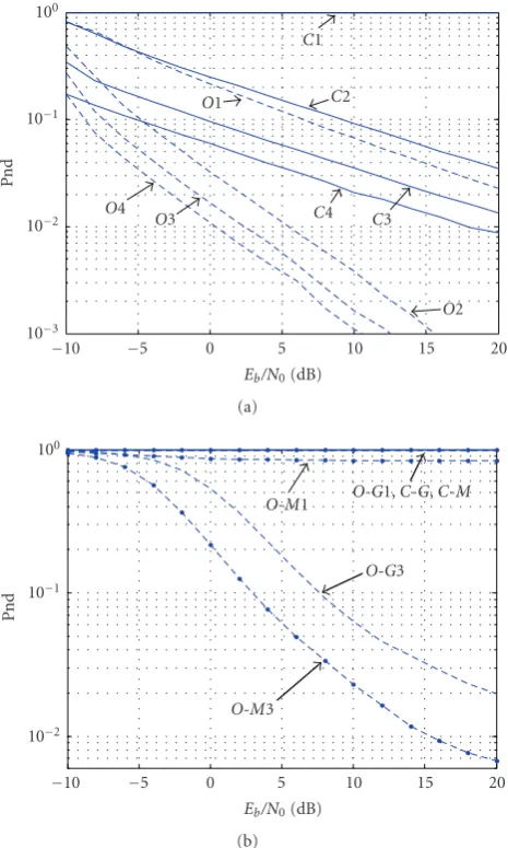
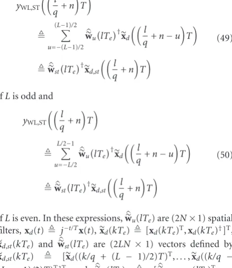
Figure4: Probability of nondetection of CONV-LS (C) and OPT-LS (O) receivers as a function of SNR,K =64,T =2Te, one
in-terference, INR = SNR + 20 dB, phase, DOA and delay random, FAR=0.001, 100 000 realizations, BPSK andN=1, 2, 3, 4 (a), MSK (M), GMSK (G),N=1,L=1, 3 (b).
are evaluated over 100 000 bursts. Under these assumptions, Figure 4(a)shows the probability of nondetection of the op-timal delayloTe by the CONV-LS (C) and OPT-LS (O)
re-ceivers as a function of the input SNR,μs2πs/η2, for a FAR
equal to 0.001 and for several values of the number of sen-sors. Note, forN = 1, the much better performance of the OPT-LS receiver due to its capability to reject the rectilin-ear interference by phase discrimination between the sources. Note, for 2≤N≤4, the better performance reached by the OPT-LS receiver, due to a better discrimination between the sources, done jointly by the phase and DOA, and despite of the fact that the CONV-LS receiver rejects the interference by a DOA discrimination. Thus, for rectilinear sources, software may replace sensors for given performances.
Note that when the interference considered previously corresponds to a useful path different from i0, the