Analysis and processing of pixel binning for color image sensor

R E S E A R C H

Open Access

Analysis and processing of pixel binning for

color image sensor

Xiaodan Jin and Keigo Hirakawa

Abstract

Pixel binning refers to the concept of combining the electrical charges of neighboring pixels together to form a superpixel. The main benefit of this technique is that the combined charges would overcome the read noise at the sacrifice of spatial resolution. Binning in color image sensors results in superpixel Bayer pattern data, and subsequent demosaicking yields the final, lower resolution, less noisy image. It is common knowledge among the practitioners and camera manufacturers, however, that binning introduces severe artifacts. The in-depth analysis in this article proves that these artifacts are far worse than the ones stemming from loss of resolution or demosaicking, and therefore it cannot be eliminated simply by increasing the sensor resolution. By accurately characterizing the sensor data that has been binned, we propose a post-capture binning data processing solution that succeeds in suppressing noise and preserving image details. We verify experimentally that the proposed method outperforms the existing alternatives by a substantial margin.

1 Introduction

Recent progress on digital camera technology has had extraordinary impact on numerous electronic industries, including mobile phones, security, vehicle, bioengineer-ing, and computer vision systems. In many applications, sensor resolution has exceeded the optical resolution, meaning that the additional hardware complexity to increase pixel density would not necessarily result in large image quality gains. The significant improvement in sen-sor sensitivity has allowed cameras to operate in lighting conditions that were unthinkable with film cameras.

Despite increased sensitivity, however, noise remains a serious problem in modern image sensors. Available tech-nologies for reducing noise in hardware include backside illuminated architecture [1,2], color filters with higher transmittance [3,4], and pixel binning [5-7]. Processing techniques at our disposal include image denoising [8-10], joint denoising and demosaicking [11-14], image deblur-ring [15,16] (long shutter to compensate for light), and single-shot high dynamic range imaging [17].

The goal of this article is to provide a comprehensive characterization of the pixel binning for color image sen-sors, and propose post-capture signal processing steps

*Correspondence: [email protected]

Electrical and Computer Engineering, University of Dayton, Dayton, Ohio, USA

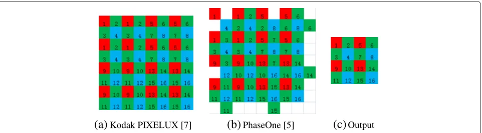
aimed at eliminating the binning artifacts. Binning refers to the concept of combining the electrical charges of neighboring pixels together to form a superpixel. The combined signal will then be amplified by a source fol-lower and converted into digital values by an analog-to-digital converter. The main benefit of this technique is that the combined charges would overcome the read noise, even if the individual pixel values are small. The improved noise performance comes at the price of spatial resolution loss, however. Binning in color image sensors is compli-cated by the presence of color filter array (CFA). Data are typically obtained via a single CCD or CMOS sensor with a CFA spatial subsampling procedure, a physical construc-tion whereby each pixel locaconstruc-tion measures only a single color. Figures 1a,b show the most well known CFA scheme called the Bayer pattern, which involves red, green, and blue filters. To maintain the fidelity of color, binning in

colorimage sensors are performed by combining

neigh-boring pixels with the same color filter. As evidenced by the two well known binning configurations shown in Figures 1a,b, the resultant superpixel form a Bayer pat-tern, as shown in Figure 1c. The subsequent demosaicking algorithm—the process of interpolating to recover the full RGB representation of the image from the CFA subsam-pled sensor data—yields the final, lower resolution, less noisy image.

(a)

(b)

(c)

Figure 1Commonly used binning schemes.Binning refers to the concept of combining the electrical charges of neighboring pixels together to form asuperpixel. (a–b) The numbers over the high resolution Bayer pattern indicate which pixels are combined together. (c) The resultant superpixel Bayer pattern, where the numbers indicate the relative locations of the combined pixels (for [7] and [5]).

However, it is a common knowledge among the practitioners and camera manufacturers that binning introduces pixelization artifacts. An example is shown in Figure 2. As will be made clear in the sequel, these artifacts differ from the ones stemming from loss of res-olution, and therefore it cannot be eliminated simply by increasing the sensor resolution. In-depth analysis of the sampling scheme implied by the binning proves that gross mismatch between binning and demosaicking results is at fault for the severe pixelization. Hence the rightway to correct this problem is to design a binning-aware demo-saicking algorithm. The proposed method still draws from the established demosaicking principles, but with pro-found differences in the way spatially high frequency components are handled. To the best of the knowledge of the authors, this is the first major article to examine pixel binning problem in color image sensors from the signal processing perspective, and to provide post-capture pro-cessing solution to correct for the pixelization artifacts.

The remainder of this article is organized as follows. We begin by briefly reviewing CFA sampling and demosaick-ing in Section 2. Section 3 provides a rigorous analysis of binning. A novel binning-aware demosaicking technique is developed in Section 4. We experimentally verify its

effectiveness in 5 before making concluding remarks in Section 6.

2 Background

2.1 CFA sampling

Thanks to the seminal work of [18] and further inves-tigations by [19-21], CFA sampling is well characterized and understood. The key insight is the two dimensional Fourier analysis of CFA sampled sensor data, which reveals that the signal is preserved by an efficient space-color representation. Specifically, let x : Z2 → R3, where x(n) =[xr(n),xg(n),xb(n)]T correspond to the

RGB tri-stimulus value at locationn∈Z2. Then the CFA subsampled data has the following form:

y(n)=c(n)Tx(n)

=c(n)T

⎡ ⎣1 1 01 0 0

1 0 1 ⎤ ⎦

⎡ ⎣0 1 01 −1 0

0 −1 1

⎤ ⎦_x(n)

=1 cα(n) cβ(n) ⎡ ⎣xxgα((nn))

xβ(n) ⎤ ⎦,

(1)

wherec : Z2 →[ 0, 1]3denotes the translucency of CFA at locationn. The advantage to the representation is that the difference imagesxα=xr−xgandxβ =xb−xg enjoy

rapid spectral decay and can serve as a proxy for chromi-nance. On the other hand, the “baseband” green image xg can be taken to approximate luminance. As our

even-tual image recovery task will be to approximate the true color image triple x(n) from acquired sensor data y(n), note that recovering either representations ({xr,xg,xb}or

{xg,xα,xβ}) are equivalent. Moreover, the representation

of (1) allows us to re-cast the pure-color sampling struc-ture in terms of sampling strucstruc-turescαandcβ associated with the difference channelsxα andxβ. For more exten-sive investigation on the bandlimitedness assumptions of {xg,xα,xβ}, see [18-20].

Denote by the uppercase letters the discrete space Fourier transforms and ω = (ω1,ω2)T ∈ {R/(2π)}2 (R/(2π)denotes the quotient group ofRby the subgroup 2πZ) the two dimensional Fourier index. Then the Fourier analysis of CFA is:

Cα(ω)= λ∈πZ2

2

δ(ω−λ)

4 ,

Cβ(ω)= λ∈πZ2

2

ej{λT(11)}δ(ω−λ)

4 ,

whereδ(·)is the Dirac delta function, andZ2denotes the cyclic group of order 2. Note that the phase shift term in Cβarises due to the relative position of blue pixels relative to the red (the origin is assumed to be on a red pixel). The corresponding Fourier analysis of the sensor dataytakes the following form:

Y(ω)=Xg(ω)+Cα(ω) Xα(ω)+Cβ(ω) Xβ(ω)

=Xg(ω)+

λ∈πZ2 2

Xα(ω−λ)+ej{λT(1₁)}_Xβ(ω−λ)

4 ,

(2)

wheredenotes convolution. The Fourier support of the resultant sensor signal is shown in Figure 3.

2.2 Demosaicking

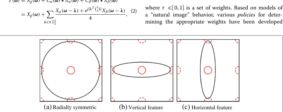
Most demosaicking algorithms described in the literature make use (either implicitly or explicitly) of correlation structure in the spatial frequency domain, often in the form of local sparsity or directional filtering [14,19,21-23]. As noted in our earlier discussion, the set of carrier fre-quencies induced bycαandcβinclude [π, 0]Tand [ 0,π]T, locations that are particularly susceptible to aliasing by horizontal and vertical edges. Figures 3b,c indicates these scenarios, respectively; it may be seen that in contrast to the radially symmetric baseband spectrum of Figure 3a, chrominance–luminance aliasing occurs along one of either the horizontal or vertical axes. However, success-ful reconstruction can still occur if a noncorrupted copy of this chrominance information is recovered, thereby explaining the popularity of (nonlinear) directional fil-tering steps [19,21-23]. We can, therefore, view the CFA design problem as one of spatial-frequency multiplexing, and the CFA demosaicking problem as one of demulti-plexing to recover subcarriers, with spectral aliasing given the interpretation of “cross talk” [19].

In order to carry out this demultiplexing, signal-adaptive demosaicking methods take the scenarios of Figure 3a–c into account. Typically, this is carried out by first filtering in both horizontal and vertical directions to yield reconstructionsxhˆ andxvˆ , respectively. Taking their convex combination to yield the final result:

ˆ

xτ(n)=τ(n)xhˆ (n)+(1−τ(n))xvˆ (n), (3)

whereτ ∈[ 0, 1] is a set of weights. Based on models of a “natural image” behavior, various policies for deter-mining the appropriate weights have been developed

(a)

(b)

(c)

Figure 3Idealized spectral support of a color image acquired under the Bayer pattern.In each figure, the horizontal and vertical axes span [−π,π)2_{of Fourier index, and the DC is located at the center of the figure. Solid lines indicate the baseband signals, while replicated spectra with}

[14,19,21-23]. For example, the weight combination should maximize the homogeneity uxˆ(n)—defined as a percentage of pixels in the neighborhood of n (denoted η(n)) that are similar tox(n)[22]:

u_xˆ(n)= #{m∈η(n):d(xˆ(n),xˆ(m)) < }

#{η(n)} (4)

whered(·,·)is some distance metric and is a tolerance parameter.

3 Analysis of binning

Let us rigorously analyze the effects that binning has on the acquired sensor data. We begin in Section 3.1 with a brief review of the signal-to-noise ratio (SNR) gains that binning is expected to improve [24]—the main motiva-tion behind binning. An in-depth analysis in Secmotiva-tion 3.2 will prove that a combination of binning and demosaick-ing results in a loss of resolution that is far worse than commonly believed. Section 3.3 offers an alternative per-spective that paves a path towards recovering artifact-free images.

3.1 Signal measurement uncertainty

There are at least three types of noise that contribute to the overall error. “Shot noise” is due to the stochasticity of the photon arrival process, and it is well modeled by Poisson distribution. The dark current stemming from in-circuit electron excitation results in “thermal noise,” whose power is proportional to the exposure time. Finally, the source follower and analog-to-digital converter introduce the homoscedastic noise that is known as the “read noise.” The overall SNR of captured image is well modeled by:

SNRpix:=20 log10(Q·t·y)−10 log10(Q·t·y+D·t+N), (5)

wheretis the exposure time,Qis the quantum efficiency constant,Dis the dark current constant, andNis the read noise power.

Owing to the fact that the image sensor resolution exceeds the optical resolution in many applications, bin-ning is an attractive way to trade off the excess spatial res-olution for gains in SNR. It is instructive first to consider summing M pixel values digitally, post-acquisition. The signalyis boostedM-fold while the noise power increases Mtimes, resulting in an overall 10 log₁₀(M)dB gain:

SNRsum:=20 log10(M·Q·t·y)

−10 log₁₀(M·Q·t·y+M·D·t+M·N) =SNRpix+10 log10(M)≥SNRpix.

(6)

Combining electrical charges of neighboring pixels to form a superpixel in hardware offers advantages over sim-ply summing pixels digitally. The main difference is that when the electrical charges are combined before source follower and analog-to-digital converter, the uncertainty due to read noise remains constant. The corresponding SNR is:

SNRbin=20 log10(M·Q·t·y)

−10 log₁₀(M·Q·t·y+M·D·t+N) ≥SNRsum.

(7)

As illustrated by the example in Figure 4, the differences between SNRbin and SNRsum are more noticeable when

the signal intensity y becomes small and read noise

N become dominant—meaning that binning is most

effective in the low light ranges.

3.2 Binning “sampling”

Due to the fact that binning combinesMelectric charges of neighboring pixels, each pixel cannot be shared by more than one superpixel. Moreover, the charges can be combined by summation only (i.e. no fractional combina-tions). As such, the options for binning schemes are fairly limited. Furthermore, the superpixels produced by pixel binning in color image sensors form a Bayer pattern that requires the additional step of demosaicking to recover the full color low resolution image. We will show that super-pixel Bayer pattern suffers from many problems that the pixel-level Bayer pattern does not, leading to the conclu-sion that combining pixel binning and demosaicking is the wrong approach.

Consider Kodak PIXELUX, the most widely used bin-ning scheme illustrated in Figure 1a,c [7]. It combinesfour neighboring pixel values together to form one superpixel.

Figure 4SNR as a function of signal intensity.Here,M=4,

This process of combining neighboring pixels to form a single superpixel is equivalent to applying a convolution operator followed by downsampling:

• filtering: lethbindenote the filter coefficients

hbin(n)= n−

1 1

+ n− ₋₁1

+ n− −1

1

+ n− −₋₁1

,

(8)

where(·)denotes the Kronecker delta function.

Then the charge summation in PIXELUX is

ybin(n)=y(n) hbin(n).

• downsampling: to yield the superpixel Bayer pattern

datas, do

s(2n)=ybin(4n)

s 2n+ 0

1

=ybin 4n+

0 1

s 2n+ 1

0

=ybin 4n+

1 0

s 2n+ 1

1

=ybin 4n+

1 1

.

(9)

Note that downsampling implied by (9) is non-uniform— the spatial relationships between samples are changed by the different relative shifts applied to each super pixels (contrast this to (11) below). The Fourier transform ofsis (derived in Appendix 2):

S(ω)≈

λ∈πZ2 2 ⎛

⎝Xα ω−λ 2

+ ej(ω2)

T₍1₁₎ unwanted filter ej λ 2 T

(1₁₎

Xβ ω−λ

2 ⎞

⎠

+

θ∈Z2 2

ej(ω2)

T_θ Hbin _ω 2 16 unwanted filter Xg _ω 2 + λ∈π

2Z24\( 0 0)

θ∈Z2 2

ej(ω2+λ)

T

θ_H bin

_ω 2 −λ

16 antialias filter Xg _ω

2 −λ

aliasing .

(10)

The corresponding Fourier support ofS(ω) is shown in Figure 5. Note that the unwanted filter will boostXgto 16

Figure 5Idealized spectral support of binning sampled data

S(ω)in (10), corresponding to Figure 1.As before, solid lines indicate the baseband signals, while spectra with the dashed lines arises as a result of CFA sampling. Black and red lines correspond to the support of luminance and chrominance images, respectively. The blue box represents the original sampling rate.

at the DC. The approximate relation above is admitted by the bandlimitedness assumptions ofXαandXβ:

Hbin(ω)Xα(ω−λ)≈4Xα(ω−λ) Hbin(ω)Xβ(ω−λ)≈4Xβ(ω−λ).

The main advantage of binning in (9) over (2) is that the signal strength of the basebandXg and the

chromi-nance componentsXαandXβare boosted by four times— consistent with the SNR analysis in the previous section. As evidenced by Figure 5a, the Fourier support of (9) closely resembles the Bayer pattern of Figure 3a. Super-pixel Bayer pattern data in (10) is far from an ideal Bayer pattern representation of the true imagex(n)we hope to recover froms(n), however. One distortion we see is the unwanted filtering term_θ∈Z2

2e jωT_θ/2

that degrades the baseband luminance/green signalXg(ω). Another

compli-cation is that the antialiasing is only partiallyeffective, allowing aliasing to corrupt the basebandXg(ω)nearω=

±[ 0,π

4]T,±[π4, 0]T,±[π4,π4]T,±[π4,−4π]T.

Contrary to the popular belief that Kodak PIXELUX binning results in 2×2 reduction in resolution, the main conclusion we draw from (9) is that the “Nyquist rate” of this binning scheme isπ/4 due to high risk of aliasing— implying that theactualresolution loss is 4×4, far worse than the presumed 2×2.Even if this Nyquist rate did not cause problems (e.g. increase sensor resolution),s does not escape the unwanted filtering term in (9)—this can-not be eliminated simply by increasing sensor resolution. Hence when a demosaicking algorithm is applied to the superpixel Bayer pattern data s, what is expected is a filtered and aliased image that we have already seen in Figure 2.

3.3 Binning “subsampling”

will provide the basis for the proposed binning-aware demosaicking algorithm. Continuing with the analysis of PIXELUX, consider Figure 6a which displays data equiv-alent to the superpixels of Figure 1c. The superpixels are placed at the center of the four averaged pixels, denot-ing the implied superpixel positions. Other locations are given 0 value. This data can be represented by applying a convolution operator followed by subsampling, as follows:

• filtering: The charge summation in PIXELUX is

ybin(n)=y(n) hbin(n).

• subsampling: to yield the binning subsampling datat,

do

t(4n)=ybin(4n)

t 4n+ 0 1

=ybin 4n+

0 1

t 4n+ 1 0

=ybin 4n+

1 0

t 4n+ 1 1

=ybin 4n+

1 1

t(n)=0otherwise.

(11)

With arithmetic, the Fourier transform oftis deduced to:

T(ω)≈

λ∈π2Z24

Xα(ω−λ)+ej{λT(11)}Xβ(ω−λ) 4

+

λ∈π

2Z24

θ∈Z2 2

ej{λTθ}Hbin(ω−λ)Xg(ω−λ)

16 .

(12)

(a)

(b)

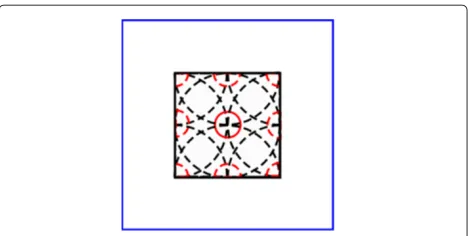
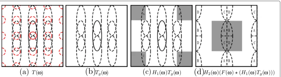
Figure 6Binning subsampling is an alternative interpretation to the binning sampling in Figure 1.(a) Subsampled datat(n)in (11) equivalent to the superpixel Bayer pattern of Figure 1c. (b) Idealized spectral support of binning subsampled dataT(ω)in (12). The baseband signalXgisfree of aliasingin the shaded region. As before, solid lines indicate the baseband signals, while spectra with the dashed lines arises as a result of CFA sampling. Black and red lines correspond to the support of luminance and chrominance images, respectively.

Note that the summation overλsuggests 16 modulations. However, exceptλ∈ π₂Z2₃, otherλresults in_θ∈Z2

2e j{λT_θ}

is 0, as shown in Figure 7. The support of this transform is illustrated in Figure 6b.aAs evidenced by this figure, the modulated baseband signal componentsXg(ω−λ)

over-lap each other almost entirely—that is, they are aliased. However, the shaded regions of Figure 6b are still free of aliasing. Indeed, this uncorrupted portion of the Fourier support is the key to post-binning processing that is the subject of next section.

4 Binning-aware demosaicking

Motivated by the analysis of pixel binning subsampling in (12), we now present a novel binning-aware demo-saicking aimed at recovering full-color image x without introducing binning artifacts. We accomplish this in three stages.

Step 1: Chrominance estimation

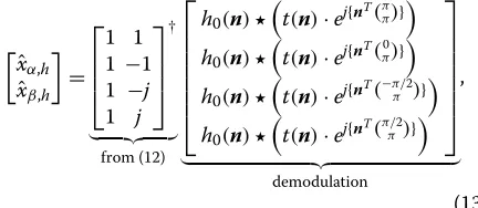
Drawing parallels to [19], we assume thatlocalimage fea-tures are either vertically or horizontally oriented (approx-imately). If this assumption holds, certain subsets of the modulated chrominances in (11) are assumed to be alias-free conditional under the vertically or horizontally ori-ented image features—this is illustrated in Figures 8a. For example, assuming horizontal feature, an amplitude demodulation recovers the desired chrominance images xαandxβ:

ˆ xα,h

ˆ xβ,h

= ⎡ ⎢ ⎢ ⎣ 1 1 1 −1

1 −j

1 j ⎤ ⎥ ⎥ ⎦ † from (12) ⎡ ⎢ ⎢ ⎢ ⎢ ⎢ ⎢ ⎣

h0(n)

t(n)·ej{nT(ππ)}

h0(n)

t(n)·ej{nT(π0)}

h0(n)

t(n)·ej{nT(−π/π2)}

h0(n)

t(n)·ej{nT(π/π2)} ⎤ ⎥ ⎥ ⎥ ⎥ ⎥ ⎥ ⎦ demodulation , (13)

where (·)† denotes a pseudo inverse matrix and h0 is a lowpass filter whose passbands matches the support ofXα andXβ. The reconstruction of vertically oriented image

Figure 7Fourier transform of_θ∈Z2

2e

j{λT_θ}

ω ω ω ω ω ω

ω ω

Figure 8Idealized spectral support of binning subsampled data, at various stages of binning-aware demosaicking.Shaded regions denote filter support. See text.

feature (denoted xˆα,v,xˆβ,v) is same as (13) but with 90°

rotation.

Step 2: Luminance filtering

Once the xˆα,h and xˆβ,h are recovered, we compute the

green imagexˆg,h. Subtracting

m∈4Z2 ˆ

xα,h(m)(m−n)+ˆxβ,h(m+

1 1

)(m+ 1 1

−n)

from subsampled binning datat(n)results a Fourier trans-form that is comprised only ofxg: (from (12))

Tg(ω)=

λ∈π

2Z24

θ∈Z2 2

ej{λTθ}Hbin(ω−λ)Xg(ω−λ)

16 .

(14)

This is illustrated in Figure 8b. To reconstruct the green imagexˆg,hfrom the unaliased (shaded in Figure 8b)

por-tions of tg, we carry out a standard demodulation, as

follows:

ˆ

xg,h=h2(n) {

modulation

f(n)· {h1(n) tg(n)

isolate unaliased }}

isolate signal

,

whereh1andh2are lowpass and highpass filters, respec-tively; andfis a sum of sinusoids intended for modulation, as follows:

H1(ω)=

1 if|ω1|> π₂ and|ω2|> π₂

0 else

H2(ω)=

1 if|ω1|< π₂ and|ω2|< π₂

0 else

F(ω)=

λ∈₍±_±π_π)/4

δ (ω+λ)

θ∈Z2 2e

j{λT_θ}.

(15)

As illustrated in Figure 8c,d, the modulation byf(n)not only shifts the spectrums, but also creates additional alias-ing copies. Hence, the filter h2 is needed to attenuate them. The same procedure can be used to find the green imagexˆg,vbased onxˆα,vandxˆβ,v.

Step 3: Directional selection

Once xhˆ = {ˆxg,h,xˆα,h,xˆβ,h} and xvˆ = {ˆxg,v,xˆα,v,xˆβ,v}

are found, they must be combined to yield the final esti-mate,xtˆ = {ˆxg,xˆα,xˆβ} via the convex combination (3). As already mentioned, the directional selection variable τ has received considerable attention in research and many techniques are available. However, these studies often lack analysis under noise—although binning reduces noise considerably, most directional selection variables are nevertheless sensitive to random perturbations.

To address the problem of directional selection under noise, we modified theτcriteria used in the popular adap-tive homogeneity directed (AHD) demosaicking method as follows:

ˆ

τ(n)=arg max

τ∈[0,1]uxˆτ(n) (16)

ˆ

xt(n)=ˆxτ (ˆn)(n), (17)

wherexˆτ andu_xˆare as defined in (3) and (4), respectively. Contrast this to the original AHD formulation which selected either xhˆ or xvˆ (i.e. τ ∈ {0, 1} instead of τ ∈ [ 0, 1]) as the final outputxtˆ . The modified strategy of (16) behaves similarly to the original AHD near the edges of an image, but encourages averaging in the flat regions of the image. It was found empirically to be far more robust to directional selection under noise.

5 Experimental validation 5.1 Setup

ˆ

xy(n), and xyˆ (n)). The first is a state-of-the-art demo-saicking method [19] applied to superpixelss(n)(i.e. out-put from PIXELUX binning):

ˆ

xs(n)=demosaicking(s(n)).

The second is the same demosaicking method [19] applied to PhaseOne binning superpixelsp(n):

ˆ

xp(n)=demosaicking(p(n)).

The third is the application of the same demosaicking method [19] to a full resolution CFA y(n) (i.e. without binning):

ˆ

xy(n)=demosaicking(y(n)).

The fourth is a simulation of a lower resolution sensor. Let x(n) denote the downsampled version of the ideal lowpassed (antialiased) image:

x_{(n)= {h}

2x}(2n). (18)

The CFA subsampled data captured by this lower resolu-tion sensor is then

y(n)=c(n)Tx(n),

wherec : Z2 →[ 0, 1]3is same the translucency of CFA used in (1). The application of the same demosaicking method [19] to lower resolution CFAy(n)is:

ˆ

xy(n)=demosaicking(y(n)).

The output images from the proposed method (xtˆ ) and the full resolution demosaicking (xyˆ ) have the same size as the original imagex. On the other hand, the conventional binning processing are based on superpixel sampling, so the pixel density ofxsˆ andxpˆ is just a quarter of the original image (same is true also forxyˆ ). Hence when we compare all results (Figures 9, 10, 11, 12, 13; Table 1), we downsam-plextˆ andxyˆ by 2×2 (in the same manner as (18)) such that all results have the same pixel density as the lower resolution imagex.

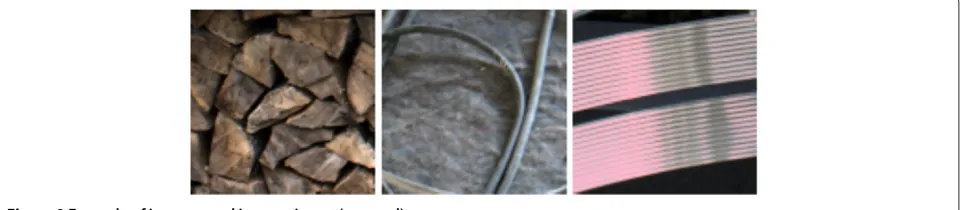
The linear images used in this simulation study are a part of the collection of [25,26], examples of which are shown in Figure 9. Numerical scores in Table 1 and Figure 13 were obtained by averaging performance over 84 images. Noise is simulated by adding pseudorandom

white Gaussian noise to the CFA datay(n), the superpixel CFA data s(n) and p(n), and the lower resolution CFA data y(n). In the experiments, the 12 bit image data in [25,26] were renormalized to ranges 0–1—meaning noise standard deviation σn = 0.01 correspond to standard

deviation of 40.96 in a 12 bit camera processing pipeline, etc. Considering the noise models in (5–7), one may ask if such a simplified noise model is appropriate. As evidenced by the analysis in (7), however, the difference between

SNR and SNRsum isM(the number of pixels combined

together); and the difference between SNRsumand SNRbin is the read noise powerN. Hence the SNR gains in binning is attributed only to the signal-independent portion of the noise, andnoton the signal dependent portion. Further-more, the read noise dominates in the low light regime. Hence simulated additive white Gaussian noise suffices for experimental verification. The binning subsample signal t(n)represents the same data ass(n)and is computed by upsamplings(n)(insert zeros where necessary).

5.2 Results

Example outputs from four different methods (xyˆ ,xyˆ , ˆ

xs,xpˆ ,xtˆ ) are shown in Figures 10, 11 and 12. As expected, demosaicking applied to a full resolution CFA (xyˆ ) has a noisy appearance due to low SNR of individual pix-els. However, edges and image features are clearly defined even after downsampling thanks to the full resolution description. Demosaicking applied to superpixel CFAs (ˆxs,xpˆ ), on the other hand, yields the opposite qualities— the noise is significantly reduced owing to high SNR of binning, but the image suffers from severe artifacts stem-ming from aliasing in (10). More specifically, the aliasing in Kodak PIXELUX binning manifests itself as a pixeliza-tion artifact, while PhaseOne binning results in zippering artifacts. However, one may argue that the aliasing arti-facts in xpˆ become less bothersome at the highest level of noise because the zippering and noise become less distinguishable. By contrast, the proposed binning-aware demosaicking method (xtˆ ) succeeds in suppressing noise while preserving the image features. Of particular inter-est is the comparison between xsˆ andxtˆ , since they both use Kodak PIXELUX binning but the proposed method

Figure 13PSNR (red/green/blue pixels are combined) of each methods, Kodak and PhaseOne refers to the binning methods of [7] and [5], respectively.Demosaicking method used for

comparison is that of [19].

Figure 14Binning sampling filtermbin(n).

yield drastically improved outcomes. Overall, the pro-posed method has better visual quality thanxsˆ andxpˆ for σn < 0.03; but proposed has a slightly noisier

appear-ance at the highest level of noise (σn = 0.03). Finally,

the output from the low resolution camera xyˆ is both robust to noise and aliasing. This is expected, as lower resolution CFA data y(n) does not share the problems that superpixel CFAsp(n),s(n),t(n)have. However,xyˆ has superior reconstruction overxyˆ without noise (σn = 0).

Table 1 Reconstruction performance in PSNR with various noise levels

Noise (σ_n) Color LR-CFA HR-CFA HR-CFA + binning

[19] [19] + DS PO + [19] K + [19] K + Proposed

0.000 R 48.1787 51.4671 45.2485 45.3275 47.8061

G 51.8147 54.7110 46.5344 47.1429 48.6259

B 46.5116 50.9532 43.6715 44.5752 45.5689

0.005 R 47.1788 46.5149 44.6596 44.7572 46.8994

G 50.1223 48.5953 46.3633 41.5903 47.6607

B 45.6221 45.2237 43.1426 43.9331 44.6091

0.010 R 45.4430 42.1931 43.4914 43.5929 45.2686

G 47.6553 43.9223 44.5383 44.9318 45.9540

B 44.0420 40.7293 42.0733 42.7001 42.9732

0.015 R 43.7677 39.1858 42.2368 42.3349 43.6632

G 45.5264 40.7919 4.18183 43.4857 44.3119

B 42.4968 37.6716 40.9172 41.4211 41.3987

0.020 R 42.2672 36.9118 41.0434 41.1293 42.2202

G 43.7388 38.4621 41.9128 42.1503 42.8488

B 41.0955 35.3795 39.8064 40,2189 39.9910

0.025 R 40.9430 35.0944 39.9375 40.0160 40.9391

G 42.2200 36.6133 40.7530 40.9454 41.5568

B 39.8450 33.5524 38.7712 39.1164 38.7417

0.030 R 39.7693 33.5816 38.9267 38.9959 39.7997

G 40.9107 35.0803.9327 39.7008 39.8595 40.4102

B 38.7310 32.0235.3426 37.8168 38.1076 37.6279

Figure 12 shows an example where none of the reconstruc-tion methods produced a satisfactory output (except for ˆ

xyunder no noise).

The performance is evaluated also in terms of peak SNR, using the downsampled version of the ideal low-passed (antialiased) image x in (18) as their reference. The results are summarized in Table 1. When there is no noise (σn = 0), ordinary demosaicking reconstructionxyˆ

and lower resolution sensorxyˆ yields the best results, as expected. However, the proposedxtˆ is a very close third, yielding comparably satisfactory results. Binning resultxsˆ is worst by far due to binning artifacts.

When noise is taken into consideration, the quality of ˆ

xysuffers greatly as expected. Even with noise variance as little asσn = 0.005, the performance ofxyˆ deteriorates

significantly, while performance of xsˆ , xpˆ , xtˆ , and xyˆ in terms of PSNR are far less sensitive to noise. With mod-erate noise levels (σn<0.03) the proposed binning-aware

demosaicking clearly outperforms the artifact-plagued demosaicking of superpixels. With the largest noise level considered (σn = 0.03), PSNR performances of xsˆ , xpˆ ,

andxtˆ are closer to each other because deteriorations in output images are dominated by noise (rather than by artifacts).

The analysis in Figures 10, 11, 12, 13 and Table 1 sheds a light on the decades-old debate about resolution versus noise. On one hand, the lower resolution sensor delivers consistent performance under noise (xyˆ ). How-ever, Figure 11 shows that under no noise, extra sensor resolution is still desirable. Consider Figure 13. The com-parison between green (low resolution) and red (high resolution) curves is consitent with the image quality of Figures 10 and 11. With the availability of pixel binning, we would compare the green curve with the “max func-tion” over the red and blue (binning) curves in Figure 13. Hence one can think of binning as a way to narrow the gap between the red and green curves in noise, with-out making sacrifices to the advantages of higher spatial resolution.

6 Conclusion

In this article, we proved via a rigorous analysis ofbinning

sampling that Kodak PIXELUX binning scheme results

in 4×4 reduction in image resolution—contrary to the popular belief that binning of four pixels should result in 2×2 reduction in resolution. We proposed a binning-aware demosaicking algorithm based on the Fourier anal-ysis ofbinning subsampling to combine unaliased copies of the Fourier spectra together via the demodulation. The resultant method succeeds in reconstructing the color image with only 2×2 resolution loss—or increas-ing the resolution by 2×2 over the traditional approach of applying demosaicking to superpixels. The binning-aware demosaicking also succeeds in suppressing noise

and preserving image details. We verified experimen-tally that the binning-aware demosaicking outperforms the alternatives.

Appendix 1: Proof of Fourier Representation of binning subsampling

We provide the proof for Equation (12). LetHbin be the Fourier transform of (8). Then the combination of charges can be represented as:

Xrbin(ω)Xr(ω)Hbin(ω)

Xgbin(ω)Xg(ω)Hbin(ω)

Xbbin(ω)Xb(ω)Hbin(ω).

Due to band limitedness of Xα and Xβ, the following approximation hold:

Xαbin(ω)Xrbin(ω)−Xgbin(ω)=Hbin(ω)Xα(ω)≈4Xα(ω)

Xβbin(ω)Xbbin(ω)−Xgbin(ω)=Hbin(ω)Xβ(ω)≈4Xβ(ω). (19)

where we used the fact thatHbin(0)=4. Define mbin(n) =

θ∈Z2

4(n − θ), as illustrated in Figure 14. The binning subsampling data t(n) refers to the concept of combining the electrial charges of four neighboring pixels together to form asuperpixel. The pro-cess is illustrated in Figure 6a. Mathmatically,t(n)can be written as:

t(n)=mbin(n)xrbin(n)+mbin n+ 1 0

xgbin(n)

+mbin n+ 0 1

xgbin(n)+mbin n+ 1 1

xbbin(n)

=mbin(n)xαbin(n)+mbin n+ 1 1

xβbin(n)

+

θ∈Z2 2

mbin(n+θ)xgbin(n).

In the Fourier domain,t(n)can be expressed as

T(ω)=Mbin(ω) Xαbin(ω)+(ej{ω T₍1_1)}

Mbin(ω)) Xβbin(ω)

+

θ∈Z2 2

ej{λTθ}Mbin(ω) Xgbin(ω)

where

Mbin(ω)=

λ∈π

2Z24

δ(ω−λ)

16 .

With arithmetic and approximation of (19), the Fourier transform oft(n)simplifies to:

T(ω)≈ λ∈π

2Z24

Xα(ω−λ)+ej{λT(11)}_Xβ(ω−λ) 4

+

λ∈π

2Z24

θ∈Z2 2

ej{λTθ}Hbin(ω−λ)Xg(ω−λ)

The Fourier support ofT(ω)is illustrated in Figure 6b.

Note that the summation over λ suggests that

bin-ning subsampling will result in 16 modulations. How-ever, _θ∈Z2

2e j{λT_θ}

is 0 for many values ofλ, as shown in Figure 7. As a result, there are only nine actual modulations.

Appendix 2: Proof of Fourier representation of binning sampling

We provide the proof for Equation (10). The binning sam-pling data s(n) refers to the concept of combining the electrial charges of four neighboring pixels together to form a superpixel Bayer pattern. The process is illus-trated in Figures 1a,c. Similar to binning subsampling (see Appendix 1, binning samplings(n)has the following rep-resentation (it is mathmatically convenint to considers(n₂) forneven, rather thans(n)directly);

sn 2

=mbin(n)xrbin(n)+mbin n+ 2 0

xgbin n+ 1 0

+mbin n+ 0 2

xgbin n+ 0 1

+mbin n+ 2 2

xbbin n+ 1 1

=mbin(n)xαbin(n)+mbin n+ 2 2

xβbin n+ 1 1

+mbin(n)xgbin(n)+mbin n+ 2 0

xgbin n+ 1 0

+mbin n+ 0 2

xgbin n+ 0 1

+mbin n+ 2 2

xgbin n+ 1 1

.

In Fourier domain,

S(2ω)=Mbin(ω)∗Xαbin(ω)+ ej

ωT(2 2)

Mbin(ω)

∗ ej

ωT₍1 1)

Xβbin(ω)

+Mbin(ω)∗Xgbin(ω)

+ ej

ωT₍2 0)

Mbin(ω)

∗ ej

ωT₍1 0)

Xgbin(ω)

+ ej

ωT₍0 2)

Mbin(ω)

∗ ej

ωT₍0 1)

Xgbin(ω)

+ ej

ωT(2 2)

Mbin(ω)

∗ ej

ωT(1 1)

Xgbin(ω)

=

λ∈π

2Z24

Xαbin(ω−λ)+ej

(ω+λ)T(1 1)

Xβbin(ω−λ) 16

+

λ∈π2Z24

θ∈Z2 2

ej{(ω+λ)TθXgbin(ω−λ)

16 .

Separating theXgbin(ω−λ)to two parts,λ= ₀

0

andλ=

₀ 0

and downsampling (2ω →ω), we have

S(ω)= λ∈πZ2

2 ⎛

⎝Xαbinω−₂λ+ej _ω+λ

2 T

(1₁₎

Xβbinω−₂λ ⎞ ⎠

4

+

θ∈Z2 2

ej(ω2)

T_θ Xgbin

_ω 2

16

+

λ∈π2Z24\( 0 0)

θ∈Z2 2

ej{(ω2+λ)

T_θ

Xgbin(ω₂−λ)

16 ,

where the 1/4 term on Xαbin and Xβbin comes from

exchanging Z2₄ with Z2₂. With arithmetic and approxi-mation of (19), the Fourier transform of s(n) simplifies to:

S(ω)≈

λ∈πZ2 2 ⎛

⎝Xα ω−λ 2

+ ej(ω2)

T₍1₁₎ unwanted filter ej λ 2 T

(1₁₎

Xβ ω−λ

2 ⎞

⎠

+

θ∈Z2 2

ej(ω2)

T θ_H bin _ω 2 16 unwanted filter Xg _ω 2 +

λ∈π2Z24\( 0 0)

θ∈Z2 2

ej(ω2+λ)

T_θ Hbin

_ω 2 −λ

16 antialias filter Xg _ω

2 −λ

aliasing

7 Endnote

a_{Filter h}

bin is a combination of highpass and lowpass. However, binning takes advantage of the fact that the sen-sor resolution exceeds optical resolution, meaninghbinis taken to be a lowpass/antialiasing filter onxg.

Competing interests

The authors declare that they have no competing interests.

Acknowledgement

This work was funded in part by Texas Instruments.

Received: 11 October 2011 Accepted: 29 May 2012 Published: 21 June 2012

References

1. H Yamanakam, Method and apparatus for producing ultra-thin semiconductor chip and method and apparatus for producing ultra-thin back illuminated solid-state image pickup device. US Patent 7,521,335 (2006)

3. J Compton, J Hamilton, Image sensor with improved light sensitivity. US Patent 2007/0024931 (2007)

4. U Barnhofer, J DiCarlo, B Olding, B Wandell, inProceedings of the SPIE. Color estimation error trade-offs, (2003), pp. vol. 5027, 263–273 5. W Borchenko, Phase One Patent Pending Sensor+Explained. http://www.

phaseone.com/Digital-Backs/P65//media/Phase%20One/Reviews/ Review%20pdfs/Backs/Phase-One-Sensorplus.ashx

6. Z Zhou, B Pain, E Fossum, Frame-transfer CMOS active pixel sensor with pixel binning. IEEE Trans. Electron. Dev.44(10), 1764–1768 (1997) 7. F Chu, Improving CMOS image sensor performance with combined pixels

(2005). http://www.eetimes.com/design/embedded/4013011/ Improving-CMOS-image-sensor-performance-with-combined-pixels 8. K Dabov, A Foi, V Katkovnik, K Egiazarian, Image denoising by sparse 3-D

transform-domain collaborative filtering. IEEE Trans. Image Process. 16(8), 2080–2095 (2007)

9. J Portilla, V Strela, M Wainwright, E Simoncelli, Image denoising using scale mixtures of Gaussians in the wavelet domain. IEEE Trans. Image Process.12(11), 1338–1351 (2003)

10. K Hirakawa, F Baqai, P Wolfe, inProc. SPIE , Electronic Imaging, vol. 7246. Wavelet-based Poisson rate estimation using the Skellam distribution , (2009)

11. L Zhang, R Lukac, X Wu, D Zhang, PCA-based spatially adaptive denoising of CFA images for single-sensor digital cameras. IEEE Trans. Image Process.18(4), 797–812 (2009)

12. K Hirakawa, T Parks, Joint demosaicing and denoising. IEEE Trans. Image Process.15(8), 2146–2157 (2006)

13. L Zhang, X Wu, D Zhang, Color reproduction from noisy CFA data of single sensor digital cameras. IEEE Trans. Image Process.

16(9), 2184–2197 (2007)

14. K Hirakawa, X Meng, P Wolfe, inIEEE International Conference on Acoustics, Speech and Signal Processing 2007. ICASSP 2007. A framework for wavelet-based analysis and processing of color filter array images with applications to denoising and demosaicing, (2007), pp. vol. 1, pp. I–597 15. R Fergus, B Singh, A Hertzmann, S Roweis, W Freeman, Removing camera

shake from a single photograph. ACM Trans. Graph. (TOG). 25(3), 787–794 (2006)

16. A Levin, P Sand, T Cho, F Durand, W Freeman, inACM SIGGRAPH 2008 papers, ACM. Motion-invariant photography, (2008), pp. 1–9

17. K Hirakawa, P Simon, inIEEE International Conference on Computer Vision. Single-shot high dynamic range imaging with conventional camera hardware, (2011), p. vol. 1

18. D Alleysson, S Susstrunk, J H´erault, Linear demosaicing inspired by the human visual system. IEEE Trans. Image Process.14(4), 439–449 (2005) 19. E Dubois, Frequency-domain methods for demosaicking of

Bayer-sampled color images. IEEE Signal Process. Lett. 12(12), 847–850 (2005)

20. P K Hirakawa, Wolfe, Spatio-spectral color filter array design for optimal image recovery. IEEE Trans. Image Process.17(10), 1876–1890 (2008) 21. J Gu, P Wolfe, K Hirakawa, in2010 17th IEEE International Conference on

Image Processing (ICIP). Filterbank-based universal demosaicking, (2010), pp. 1981–1984

22. K Hirakawa, T Parks, Adaptive homogeneity-directed demosaicing algorithm. IEEE Trans. Image Process.14(3), 360–369 (2005)

23. L Zhang, X Wu, Color demosaicking via directional linear minimum mean square-error estimation. IEEE Trans. Image Process.4(12), 2167–2178 24. T Fellers, K Vogt, M Davidson, CCD signal-to-noise ratio. http://www.

microscopyu.com/tutorials/java/digitalimaging/signaltonoise/ 25. P Gehler, C Rother, A Blake, T Minka, T Sharp, inProceedings of the IEEE

Computer Society Conference on Computer Vision and Pattern Recognition. Bayesian color constancy revisited, (2008)

26. L Shi, B Funt, Re-processed Version of the Gehler Color Constancy Dataset of 568 Images. http://www.cs.sfu.ca/colour/data/

doi:10.1186/1687-6180-2012-125

Cite this article as:Jin and Hirakawa:Analysis and processing of pixel bin-ning for color image sensor.EURASIP Journal on Advances in Signal Processing

20122012:125.

Submit your manuscript to a

journal and benefi t from:

7 Convenient online submission 7 Rigorous peer review

7 Immediate publication on acceptance 7 Open access: articles freely available online 7 High visibility within the fi eld

7 Retaining the copyright to your article