Design and Realization of a Safe Control System for a Parallel Manipulator

University of

Twente

Faculty of Electrical Engineering,

Mathematics & Computer Science

Design and Realization of a Safe Control

System for a Parallel Manipulator

M. Eglence

M.Sc. Thesis

Supervisors: prof. dr. ir. J. van Amerongen

dr. ir. T.J.A. de Vries

dr. ir. J.F. Broenink

ir. B.J. de Kruif

June 2003

Report Number

010CE2003

Control Laboratory

Faculty of Electrical

Engineering,

Mathematics &

Computer Science

iii

Abstract

The Control Laboratory at University of Twente has purchased

an Imotec

xyz

-manipulator. The manipulator is delivered with

an open operating system. This thesis treats the design and

realization of a safe guarded controller system for the Imotec

manipulator. Safety issues are discussed to make the

manipulator operate safely for doing research experiments by

students and staff. This concerns safety of the manipulator

itself and of the people working with it. The first experiments

will be concerned with the research on Learning Feed Forward

Control (LFFC).

The safe guarded controller system is implemented as a Multi

Agent Controller (MAC) system. The controller is tested in

simulation (20-Sim) and has proven to work correctly.

The designed controller has largely been implemented on the

real system and has been found to work according to

expectations. For a slow, large stroke movement, a maximum

tracking error of 250 [µm] was found at moments of velocity

reversal; otherwise, the max tracking error amounted 100 [µm].

Because of time constraints, the experiments with LFFC have

not been carried out.

v

Acknowledgements

Thanks go out to a lot of people who made it possible for me to

graduate. First of all, I would like to thank my family for their

never-ending support and encouragement.

I would like to thank my supervisors who gave me the

opportunity to work on this interesting thesis. Especially I

would like to thank Theo de Vries for his valuable guidance

and tips during the thesis, the good time we had at Imotec and

for the great fun we had with testing the robot.

Herman, Jan, Peter and Richie thanks for the good time and

interesting discussions at Imotec.

Job van Amerongen I would like to thank for the opportunity to

graduate at the Control Laboratory.

Last but certainly not least I would like to thank the lady that

made my life so much nicer by stepping in to it. Sabire, thanks

for your love and encouragement.

Enschede, June 2003

vii

Table of contents

1 I

NTRODUCTION

... 1

1.1 B

ACKGROUND

... 1

1.2 L

EARNING

F

EED

-F

ORWARD

C

ONTROL

... 1

1.3 T

HE

I

MOTEC MANIPULATOR

... 2

1.4 T

HE ASSIGNMENT

... 4

1.5 T

HESIS

S

TRUCTURE

... 4

2 D

ESIGN CONCERNING SAFETY ISSUES

... 5

2.1 I

NTRODUCTION

... 5

2.2 M

ALFUNCTIONING OF THE MANIPULATOR

... 5

2.2.1 C

HECKING THE MECHANICAL STRUCTURE

... 5

2.2.2 C

HECKING THE POWER SUPPLY

... 12

2.2.3 C

HECKING THE LINEAR MOTORS

... 12

2.2.4 C

HECKING THE MOTOR AMPLIFIERS

... 12

2.2.5 C

HECKING THE INTERFACE CARDS

... 12

2.2.6 C

HECKING THE COMPUTER SYSTEM

... 13

2.3 F

AULTS BY THE ENVIRONMENT

... 14

2.4 A

PPLIED CHECKS AND THEIR RESPONSES

... 14

3 I

MPLEMENTATION OF THE SAFE CONTROLLER SYSTEM

... 15

3.1 I

NTRODUCTION

... 15

3.2 P

OSSIBLE IMPLEMENTATION METHODS OF THE SAFE CONTROLLER SYSTEM

... 15

3.3 T

HE CONCEPT OF

MAC

SYSTEMS

... 16

3.3.1 C

ONTROLLER AGENTS

... 16

3.3.2 S

ENSOR AGENTS

... 17

3.3.3 A

CTUATOR AGENTS

... 17

3.4 C

OORDINATION OF AGENTS

... 17

3.5 MAC

SYSTEM FOR THE MANIPULATOR

... 18

3.5.1 S

TARTUP AGENT

... 19

3.5.2 A

LARM AGENT

... 20

3.5.3 G

UARDED

E

MERGENCY AGENT

... 20

3.5.4 G

UARDED

S

TANDARD AGENT

... 20

3.5.5 M

ODE

S

WITCH

C

ONTROLLER AGENT

... 21

3.6 T

OTAL OVERVIEW OF THE

MAC

SYSTEM

... 23

4 P

ATH GENERATION

... 25

4.1 I

NTRODUCTION

... 25

4.2 T

OOLS FOR PATH SPECIFICATION

... 25

4.3 T

HE

P

ATH

G

ENERATOR

... 26

4.4 T

RAPEZOIDAL PROFILE ALGORITHM

... 28

4.5 S-

CURVE PROFILE ALGORITHM

... 30

4.6 S

TRAIGHT LINE MOVEMENT

... 32

4.7 A

RC MOVEMENT

... 33

4.8 A

SSIGNING THE SAMPLE REFERENCE POINTS TO THE ARC MOVEMENT

... 34

viii

5.1 I

NTRODUCTION

... 37

5.2 D

ESIGN OF DEMONSTRATOR PATH

... 37

5.3 T

HE

20-

SIM MODEL OF THE MANIPULATOR

. ... 38

5.4 V

ERIFYING THE STANDARD MODE IN SIMULATION

... 39

5.5 V

ERIFYING THE

E

RROR

G

UARD

... 41

5.6 V

ERIFYING THE EMERGENCY SITUATION IN SIMULATION

... 42

5.7 V

ERIFYING THE ALARM MODE IN SIMULATION

... 43

5.7 E

XPERIMENTAL RESULTS

... 44

6 C

ONCLUSIONS AND RECOMMENDATIONS

... 47

6.1 C

ONCLUSIONS

... 47

6.2 R

ECOMMENDATIONS

... 48

A

PPENDIX

A: W

ORKING PRINCIPLE AND DRIVE OF LINEAR MOTOR

. ... 49

A

PPENDIX

B: H

ARDWARE OVERVIEW OF THE MANIPULATOR

... 51

A

PPENDIX

C: A

N INTRODUCTION TO

XML ... 53

A

PPENDIX

D: C

ONTROLLER SETTINGS

... 57

A

PPENDIX

E: M

ANIPULATOR

MAC

SYSTEM CODE

... 59

Introduction

1

1 Introduction

1.1 Background

At the Control Engineering Laboratory of the University of Twente (UT) research is done on

Mechatronic Systems in general and in particular on the role of the controller in it. An ongoing

project is concerned with Learning Feed-Forward Control (LFFC) [De Kruif, 2003]. To carry

out experiments for this research, an

xyz

-manipulator with parallel kinematical configuration has

been purchased by the UT. The manipulator has been developed and built by the company

Imotec, which is also a sponsor of the research. The manipulator has been delivered with an

open controller system, in order to make it possible to implement advanced control and

identifications algorithms. The first research on the manipulator will be concerned with the

application of modern function approximators in closed loop control. When doing research,

people will work closely with the manipulator. Therefore, safety is an important issue. The

manipulator should operate in a safe manner without causing danger for people working with it

and without causing damage to itself.

1.2 Learning Feed-Forward Control

For obtaining good performances with classical control systems, the parameters of the controlled

plant need to be known well. Not knowing the plant parameters accurate enough result in not

entirely knowing the dynamics of the plant. In many control problems, the plant is given as a

model of which the parameters are not known exactly. The reasons for this are various, for

instance:

Low-precision production processes make the fabricated part to differ from the

specification.

Manufacturing tolerances lead to a spread in dynamic behaviour.

Complexity of the plant makes parameter estimation difficult.

Changes in plant characteristics as time proceeds.

Non-linear effects like friction and cogging.

In many applications the goal is to come to a high precision servo system with low price

components. In these situations the classical feedback controller demerits. However, the

principle of LFFC can offer a solution [Velthuis, 2000],[Starrenburg

et al

, 1995]. In figure 1.1 a

control loop is given in which a learning component is included in the feed-forward path. In this

case, this component is a function approximator (FA).

2

The function approximator realizes an input-output mapping gained by experience. The

mapping summarizes the examples by a function. This function for instance can be the force that

is needed to compensate for the friction loss depending on the velocity of the mechanical setup.

In the depicted control loop, the feedback controller is needed for stability of the closed loop

system and to present samples for the learning mechanism of the function approximator. The

function approximator approximates the inverse dynamics of the plant based on the output of the

feedback controller. After learning, it compensates for the non-linear state dependent behavior

of the plant.

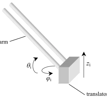
1.3 The

Imotec

manipulator

The Imotec manipulator, of which a sketch is given in figure 1.2, is a simplified Stewart

platform with three degrees of freedom namely

x

,

y

and

z

. It is driven by three Tecnotion linear

motors in vertical direction. For working principle and drive of linear motors, see Appendix A.

For an overview of the manipulator hardware see Appendix B.

Introduction

3

A set of arms in parallelogram construction attached to the translators of the motors, holds a

platform, which is the end-effector of the manipulator. The joints of the arms allow movement

only in

φ

and

θ

direction, whereas the translators only move in

z

direction (see figure 1.3). This

altogether results in an

x

,

y

,

z

motion of the platform. The parallelogram construction of the arms

restricts rotational movements of the platform. The three arms together also keep the platform in

the horizontal plane.

The manipulator has a safe work area that is shaped as a cylinder with radius 200 [mm] and

height 250 [mm]. Although the end-effector of the manipulator can exceed the dimensions of the

cylinder, it is not recommended because this will cause overloading of the leaf springs from the

joints. Specifications of the manipulator are:

Max Payload

5 [kg]

Max Speed

1 [m/s]

Max Acceleration

30 [m/s

]

Max Stroke Lin. Motor 520[mm]

The manipulator is given in its functional blocks in figure 1.4. The setup can be divided in three

major parts:

The computing system

The electrical circuitry and components

The mechanical setup.

φ

θ

z

arm

translator

4

1.4 The

assignment

The electrical circuitry and mechanical setup of the manipulator have been realized and tested.

To become operational, the manipulator’s computing system needs to be programmed. This

means that the right actions need to be taken depending on the signals from the electro-cabinet

and on user input. The objective of the assignment is to develop and realize a safe control

system. This incorporates the following points:

Design and realization of a safeguard system to make it possible to carry out experiments

with the manipulator without danger for the environment and for the setup itself.

Design of a generally applicable tool for path specification of manipulators.

Implementation of the path specification tool for the parallel kinematical

xyz

-manipulator, including setpoint generation.

Implementation of a relatively simple closed loop control system in which a modern

function approximator is integrated.

1.5 Thesis

Structure

After this introduction, in chapter 2 safety issues concerning the manipulator will be discussed.

In chapter 3 these safety issues will be implemented for the Imotec manipulator. In chapter 4,

path generation in general for manipulators will be discussed. The path generator specific for the

xyz

-manipulator will also be developed in this chapter. In chapter 5 simulations and

experimental results will be discussed. Finally in chapter 6, the conclusions and

recommendations are presented.

Design concerning safety issues

5

2 Design concerning safety issues

2.1 Introduction

Safety concerns two major aspects in manipulators. First and most important is the safety of

people operating and working with the manipulator. Second, the manipulator should not damage

itself by some motion. Usually manipulators are placed in industrial environments where people

do not work closely nearby the manipulator. In case of the Imotec manipulator, people will work

close to the manipulator when doing research. Therefore considerable attention will be paid to

human safety. The manipulator is used for doing research in the field of control engineering. It

is imaginable that a bad controller setting (unstable) can cause unsafe situations. This chapter

deals with the measures that can be taken to make the manipulator operate safely. There are two

major causes that can lead to dangerous situations in case of the manipulator.

Malfunctioning of a component of the manipulator itself.

Irresponsible behavior of people in the environment.

First the possible faults of the manipulator itself will be discussed and then faults that can arise

by the environment. Measures to handle these situations will also be discussed.

2.2 Malfunctioning of the manipulator

The Imotec manipulator consists of six basic parts, which can all lead to faults:

The mechanical structure

The linear motors

The motor amplifiers

The power supply

The interface cards

The computer system

These parts will be discussed subsequently in the next sections.

2.2.1 Checking the mechanical structure

6

the mechanical structure to break apart. This can be done by assuring that the manipulator

operates in its safe work area. The encoder readings from the linear motor can be used to

determine the position of the platform. This means that the forward kinematics of the

manipulator has to be known. The Imotec manipulator has complex forward kinematics due to

its parallel configuration. However, the inverse kinematics can be derived easily. When z1, z2

and z3 are the positions of the translators in z direction, then the following holds:

2 2 2

1 1 1

2 2 2

2 2 2

2 2 2

3 3 3

(

)

(

)

(

)

(

)

(

)

(

)

o o o

z

l

x x

y y

z z

z

l

x x

y y

z z

z

l

x x

y y

z z

= −

− −

−

−

+ +

= −

− −

−

−

+ +

= −

− −

−

−

+ +

[2-1]

Where

l

is the known length of the arms and x, y, z are the coordinates of the moving platform.

x1 is the x position of the translator 1 and y1 its y position. Note that the translators only move in

z direction, therefore xi and yi are fixed and known. zo is the initial height of the platform in z

direction when the translators are all in the bottom position (zi = 0, i = 1,2,3) . zo is calculated as:

2 2

o

z

=

l

−

r

[2-2]

Where

r

is the known radius of the circle in which the translators are aligned, see figure 2.1.

x

y

z

r

Translator 1

Translator 2

Translator 3

Fig. 2.1 Orientation and setup of the translators.

Platform

(x1, y1)

Design concerning safety issues

7

Equations [2-1] represents the inverse kinematics of the manipulator. We are interested in the

forward kinematics, i.e., we wish to regard [2-1] as three simultaneous equations with three

unknowns, (x, y, z). However, this problem cannot be solved explicitly because of its

complexity; the root function in [2-1] makes this hard. Therefore, an approximation is done [De

Kruif], to remove the root function. First a transformation is done from Cartesian coordinates to

cylindrical coordinates by using the following coordinate change:

sin( )

cos( )

x

p

y

p

z z

φ

φ

=

=

=

[2-3]

Where p is the distance between the origin and the position of the platform in the x-y plane. As

stated earlier the manipulator has a safe work area of cylindrical shape with radius 200 [mm]

and height 250 [mm]. Therefore the distance p may not exceed 200 [mm]. Hence, we can

reformulate the safety check as solving [2-1] and [2-3] for p and checking it for the given limit.

Using the coordination transform of [2-3] in [2-1] results in:

2 2 2

1

2 2 2

2

2 2 2

3

2

cos( )

2

2

cos(

)

3

4

2

cos(

)

3

o

o

z

l

r

p

pr

z z

z

l

r

p

pr

z z

z

l

r

p

pr

z z

φ

φ

π

φ

π

= −

− −

−

+ +

= −

− −

−

+

+ +

= −

− −

−

+

+ +

[2-4]

We introduce an intermediate function:

2 2 2

( , )

2

cos( )

f p

φ

=

l

− −

r

p

−

pr

φ

[2-5]

In [2-4] the root function f(p,

φ

) is still present. A plot thereof is given in figure 2.2.

8

From the plot can be seen that f(p,

φ

) has its minimum and maximum on the line where p = pmax

= 200 [mm]. With l = 541[mm], r = 300[mm] and

φ

= −

[

π π

, ]

given, we can derive:

0.20659

≤

f p

( , ) 0.53167

φ

≤

[2-6]

f(p,

φ

) can be converted into f(x) by stating:

( , )

( )

f p

φ

f x

=

x

[2-7]

with

2 2 2

2

cos( )

x l

= − −

r

p

−

pr

φ

[2-8]

and

2 2

min max

[

,

] [0.20659 ,0.53167 ] [0.0427, 0.2827]

x

∈

x

x

=

=

[2-9]

A plot of f(x) is given in figure 2.3.

By doing a linearization, f(x) can be approximated. The approximation is given by the dashed

line in figure 2.3. This line is described by:

i

min min

max min

( )

( )

( )

( )

( )

f x

f x

(

)

f x

f x

f x

x x

x

x

−

≈

=

+

−

−

[2-10]

Design concerning safety issues

9

And with the known values filled in:

i

f x

( ) 1.355

=



l

− −

r

p

−

2

pr

cos( )

φ



+

0.149





[2-11]

Substituting equation [2-10] as approximation for f(p,

φ

) into equations [2-4] gives:

2 2 2

1

2 2 2

2

2 2 2

3

1.355

2

cos( )

0.149

2

1.355

2

cos(

)

0.149

3

4

1.355

2

cos(

)

0.149

3

o

o

z

l

r

p

pr

z z

z

l

r

p

pr

z z

z

l

r

p

pr

z z

φ

φ

π

φ

π





≈ −



− −

−



+ + −





≈ −



− −

−

+



+ + −









≈ −



− −

−

+



+ + −





[2-12]

Adding up the equations in [2-12] results in (note that the cosine parts add up to zero):

2 2 2

1 2 3

3 1.355(

) 3

3

0.447

z

+ +

z

z

≈ − ⋅

l

− −

r

p

+

z

+

z

−

[2-13]

From which it follows that:

2 2 2 1 2 3

1.355(

)

0.149

3

z

z

z

z z

+

≈

l

− −

r

p

+

+ +

+

[2-14]

Combining the first equation of [2-12] with [2-14] gives:

2 2 2 2 2 2 1 2 3

1

1.355

2

cos( )

1.355(

)

3

z

z

z

z

≈ −





l

− −

r

p

−

pr

φ





+

l

− −

r

p

+

+ +

[2-15]

From which for z1 is obtained:

2 3 1

4.065

cos( )

2

z

z

z

≈

pr

φ

+

+

[2-16]

Equally for z2 the following can be derived:

1 3 2

2

4.065

cos(

)

3

2

z

z

z

≈

pr

φ

+

π

+

+

[2-17]

The equations [2-16] and [2-17] can be generalized into:

cos( )

2

cos(

)

3

A

A

α

φ

β

φ

π

=

=

+

[2-18]

For which a general solution can be found with the use of Maple as:

2 2

4

4

4

3

3

3

10

With 4.065

A

=

pr

,

2

z

z

z

α

= −

+

and

2

2

z

z

z

β

=

−

+

, the following expression is found for

the approximation of the radius:

2 2 2

1 1 2 1 3 2 2 3 3

0.246

p

z

z z

z z

z

z z

z

r

=

−

−

+

−

+

[2-20]

In figure 2.4 a plot is given of the actual radius of the platform and the approximation of it

according to [2-20].

From the plot can be seen that the approximation that is made, varies between 175 [m] and 220

[mm] depending on

φ

for p = 200 [mm]. The error that is made is given in figure 2.5.

The threshold value of the safety system to take action should be set at 170 [mm]. The platform

then can move up to a radius of 200 [mm] depending on

φ

.

Fig. 2.4 Approximation of the radius according to [2-20].

Design concerning safety issues

11

Also the z direction of the platform has to be checked to ensure that the platform does not

exceed the cylindrical work area. The height of the platform has to be determined the most

accurate in the position where it is at the edge of the radius of his work area, that means

200

p

≈

[mm] and

z

≈

0

or

z

≈

250

[mm]. In this positions the spring leafs of the joint are

bended the most.

With equation [2-13] and the approximation for the radius [2-20] the following can be stated:

2 2 2

1 2 3

3 1.355(

) 3

3

0.447

z

+ +

z

z

= − ⋅

l

− −

r

p

+

z

+

z

−

[2-21]

With the known values filled in, this results in the approximation for checking the z direction of

the platform:

2 2 2

1 2 3

1.355(

)

0.149

3

appr appr o

z

z

z

z

=

+ +

+

l

− −

r

p

− +

z

[2-22]

In figure 2.6 a plot is given of the actual z-position of the platform and the approximation of this

position according to [2-22].

From the plot can be seen that the approximation for z-position makes an under-estimation. The

error that is made is given in figure 2.7.

Fig. 2.6 Approximation of the z-position according to [2-22].

12

In the error plot can be seen that in the situation that p is zero, that means the platform is in the

centre of his work area circle, the error is the largest and has a value of 26 [mm]. In the situation

that the platform is at the edge of the safe work area (p = 200 [mm]), the error is 16 [mm]. That

means that if the threshold value of the safety system is set to 250 [mm], the platform can move

up to a height of 266 [mm] in the situation that p = 200 [mm]. Therefore the threshold value

should be set at 234 [mm]. The platform cannot move above 250 [mm] then.

2.2.2 Checking the power supply

The Imotec manipulator is fed via an Uninterruptible Power Supply (UPS). This UPS is able to

supply power to the manipulator for at least 10 seconds in case of a power break down from the

supplier net. This should give time enough for bringing the end effector to a safe situation and

shutting down the computing system. In case of a power down situation, the computing system

is alarmed via a relay that checks whether the power supply from the net is present. This should

trigger an appropriate control action.

2.2.3 Checking the linear motors

Linear motors based on permanent magnets are robust and reliable because no transmissions are

needed to transform in a linear motion. However, the linear motor still can malfunction. For

instance, the coils of the translators can heat up too much. Therefore the translators are equipped

with thermal resistors to measure the temperature. This temperature can be checked by the

computing system and in case of overheating measures can be taken. Another failure that can

occur is that the linear motor gets stuck. This can be detected by a growing tracking error and

measures can be taken.

2.2.4 Checking the motor amplifiers

The used amplifiers for the Imotec manipulator have safety checks built in. In case of faults,

outputs are set high that can be noticed by the computing system and measures can be taken. In

case of malfunctioning of the amplifiers the tracking error will become too large, this can be

detected and measures can be taken. The amplifiers can check for under/over voltage of the

power supply, short circuiting of motor currents and overheating of the amplifiers themselves.

2.2.5 Checking the interface cards

The Imotec manipulator uses three types of interface cards in the computer system: an encoder

card, a digital input/output card and an analogue output card. These can all malfunction.

Malfunctioning of the encoder card can be detected by the following.

•

The value of the encoder reading does not change at all, thus a growing tracking error.

•

The difference in values between two successive samples is much bigger then the

Design concerning safety issues

13

It is difficult to check the analogue output card directly. A feasible method is to compare the

error signal of the controller inside the software with a threshold. For instance, if the analogue

card would malfunction it either send zero to the output or a fixed value different from zero. In

both cases the translators will not move because there is no commutation performed. The

tracking error will grow large and this can be detected. Performing the commutation inside the

software and not in the amplifiers makes the manipulator inherent safe.

The digital I/O card can be checked by using redundancy. This means using two input channels

to read in one signal. For faultless operation the two inputs should be the same. But this method

costs a lot of inputs and will not be used. The faulty operation of the digital I/O card will not

cause life-threatening situations because emergency stops are not handled in software only, but

are also applied directly to a safety relay. Therefore no checks will be applied to the digital I/O.

2.2.6 Checking the computer system

With the computer system there are two types of faults possible. First it is possible that there is a

bug in the software. This can be a bug in the controller software but also a bug in the operating

system itself. It is hard to detect this kind of software problems. A bug can result in the sitation

that the tracking error will grow large during a motion or that the manipulator does not react on

commands like start and stop.

Secondly the computer can crash totally. This can be detected by means of a watchdog. This is a

hardware component, which receives a signal from the computer system and checks if the

computer is running. If the computer has crashed, this signal will not be detected and the

watchdog will notice the malfunctioning of the computer system. Then proper action can be

taken by the hardware, like activating the safety relay. In figure 2.8 the circuitry is given for the

watchdog function.

The working principle is as follows. A pulse train from the software drives a switch that

activates timer relays K1 and K2. These are of the delayed fall-off type. As long as a pulse train

is present with a period time that is smaller than the fall-of time, the contacts K1 and K2 will not

PC

+24V

GND

K1 K2

K1

K2

Safety

Relay

14

fall-off. When the computer system crashes, the pulse train will stop and after the delay time of

the relay, the contact K1 or K2 will fall-off. This will cause the safety relay to take action.

2.3 Faults by the environment

For safe operation of the manipulator, the system should not interact with the environment

physically. The Imotec manipulator is covered with a removable transparent security hedge

made of lexan. Safety switches mounted on the hedge secure operation of the manipulator only

when the hedge is mounted. This hedge ensures that no people or animals can enter the work

area of the manipulator during operation. It also provides protection against the possibility that

objects are thrown out of the work area by the manipulator.

Another cause of possible faults can be wrong input of the user. The user can cause the

manipulator to operate beyond its limits either by mistake or on purpose. The method discussed

in 2.2.1 avoids operating the manipulator beyond the limitations even if the input is wrong.

2.4 Applied checks and their responses

In section 2.2 and 2.3 possible faults that can arise have been discussed. Table 2.1 summarizes

the checks and their responses for the manipulator.

Check: What

Check: How

Response

Manipulator checks

Motor temperature

Thermal resistors to digital input

Steering signals zero

Amplifiers

Judging tracking error

Steering signals zero

Encoder cards

Judging tracking error

Steering signals zero

Computer system

Watchdog circuitry (hardware)

Power cut-off

User input

Exceeding work area

Judging end-effector position

Steering signals zero

Actuator saturation

Judging tracking error

Steering signals zero

Environment

Entering work area

Sensor on hedge (also hardware)

Power cut-off

Emergency

Emergency stop button to digital input

and to hardware

delayed power cut-off

Emergency stop and

Most of the safety checks will respond with setting the steering signals to zero if a fault arises.

The check of the computer system and entrance of the work area is handled in hardware. The

power is cut off by the safety relay that falls off. The remaining checks will be solved in

software. The next chapter describes the implementation of the safety checks and the total

controller system.

Implementation of the safe controller system

15

3

Implementation of the safe controller

system

3.1 Introduction

Implementation of the controller with all the safeguards in software can be done conveniently by

using a high level programming method. This section discusses the several implementation

options that are considered. From these options a choice will be made for the final

implementation of the safe controller system.

The purpose of the implementation method is to create a complete working controller program

with al the mentioned safety check mentioned in the previous chapter. The program must

operate on the computing system of the manipulator, but it is not a requirement that the program

must be developed on this system self.

There are some additional requirements that the used implementation form has to meet:

The software used must be able to work on a PC under DOS, because that’s the

operating system used in the manipulator. The preferred programming language is C++.

The reason for this is that C++ is an object orientated and fast programming language.

Also the Control Laboratory is experienced with C++.

Testing the created software by means of simulation before implementing it has large

advantages. Therefore, it is highly preferable that the software environment has an easy

way of doing simulations.

3.2 Possible implementation methods of the safe controller system.

The first and most obvious option is to write code in C++. This is not a high level method and

will be laborious. Also, doing tests with the created code by simulations is not easy. A better

method is the concept of agent based controller systems as proposed by [Van Breemen, 2000].

This method is more structured than a general programming language. It allows incremental

design, which means that functionalities can be added later on without interfering with earlier

implemented parts. This is very suitable for the safe controller design.

An agent is an abstract entity that is able to solve a particular part of a total complex problem.

Cooperation of multiple agents provides a solution to the total complex problem. For the present

context, this is referred as a Multi Agent Controller system (MAC). In [Bajracharya, 2003] an

integrated design tool for Multi Agent Controller systems (IDITMAC) is developed. This tool

also makes it easy to test the created software by simulation. A Dynamically Linked Library

(dll) file is created, which can be incorporated with 20-Sim modeling and simulation

16

3.3 The concept of MAC systems

The term agent is widely used in the field of software engineering and artificial intelligence.

In [Franklin, Graesser, 1997] an autonomous agent is defined as:

“An autonomous agent is a system situated within and a part of an environment that senses that

environment and acts on it, over time, in pursuit of its own agenda and so as to effect what it

senses in the future.”

Stated in other words, an agent can decide for it self whether it should undertake some actions.

To undertake the action, the agent first has to become active.

A MAC system consists of three basic agents:

Controller agent

Sensor agent

Actuator agent

In figure 3.1 the symbols that are used for the basic agents are given. The next sections will give

the explanation and describe the function of the various parts.

3.3.1 Controller agents

Two types of controller agents can be distinguished in the MAC system.

Elementary agent

Composite agent

The elementary agent is the fundamental agent of a MAC system. It implements the local

control solution for a part of the global control problem. The composite agent is a pool that

consists of elementary and/or other composite agents. This allows hierarchical organization of

the MAC system. The overall agent that contains all the other agents and is responsible for the

total control system is called a Main agent. This is also a composite agent.

Actuator

Agent

Controller Agent

Fig. 3.1 Symbols of the basic agents in a MAC system.

Implementation of the safe controller system

17

3.3.2 Sensor agents

The sensor agent senses the environment and presents the data to the other agents. The data from

the environment can be user input for controlling the system, measured values from the plant

and disturbances. Because of the discrete implementation, the data will come from Encoder

interface cards, A/D converters and digital inputs cards.

3.3.3 Actuator agents

Actuator agents present the processed control data to the environment. This control data can be

signals for indicator lights, steering signals for the plant etc. The data will be presented to the

environment by D/A converters and digital output cards.

3.4 Coordination

of

agents

Coorperation of agents is determined by a coordination mechanism. Agents that are cooperating

are combined in a pool of agents (which is a composite agent). A coordination object that is also

included in the pool does the coordination. In figure 3.2 the symbol of coordination objects is

given. The coordination objects can be divided in three types:

Independent

Cooperative

Competitive

Independent

: coordination allows two or more agent to be active at the same time. The agent

that are active at the same time have control over different outputs and do not interfere with each

other. An independent type coordination is the Parallel coordination object, which is also the

default one.

Cooperative

: coordination also allows two or more agent to be active at the same time. But now

the agent can have control over the same output. Also the output of one agent can be the input of

the other ones. Master-slave coordination object and Fuzzy addition coordination objects are

cooperative type objects.

o

Master-slave coordination: If one agent is active the other one is also active.

o

Fuzzy addition coordination: The shared output is a function of the agent outputs that are

active.

Competitive

: coordination allows only one agent to have control over a certain output.

Coordination object of this type are Fixed priority coordination, Sequential coordination and

Cyclic coordination.

o

Fixed priority coordination: From all the agents that wants to be active, the one with the

highest priority is allowed to be active.

18

o

Cyclic coordination: this coordination is almost the same as Sequential except that if the

last one in the order stops being active, the first one becomes active again.

With these four coordination objects and the possibility for a hierarchical organization, complex

controller problems can be solved in a partial manner. The MAC system for the Imotec

manipulator will be described in the next section.

3.5 MAC system for the manipulator

An overview of the total controller agents for the Imotec manipulator will be given and their

functions will be discussed. The entire controller is called the OverallController and has input

connections to the buttons like START, STOP and EMERGENCY. Also the three encoder

values

z

,

z

,

z

and the end switches of the motors are acquired by the inputs sensors. The

outputs of the OverallController are the control voltages that drive the amplifiers and the digital

outputs signals. A schematic overview of the total control system is given in figure 3.3.

The OverallController consists of a pool with a Startup, Alarm, GuardedEmergency, and a

GuardedStandard agent. The coordination is fixed priority, see figure 3.4. In the following

sections the function of these agents will be discussed.

Fig. 3.2 Symbol of the coordination objects.

Fig. 3.3 The Main controller agent for the manipulator.

Outputs

Inputs

OverallController

Implementation of the safe controller system

19

3.5.1 Startup agent

The first agent in priority order is the Startup agent. It becomes active when the ENABLE

button is pressed. This button also activates the safety relay. When active, this agent performs

the alignment and the homing of the manipulator. At the end of the homing procedure, the

platform is positioned in the lowest centre point of the safe work area cylinder, see figure 3.5.

This point is referred as the home location. The manipulator is now ready for operation and

waiting to perform a specified motion.

Fig. 3.4 Pool with agents of the OverallController system.

Fixed

OverallController

Startup

Alarm

Inputs

Outputs

voltage

voltage

Guarded

Emergency

Guarded

Standard

voltage

voltage

20

3.5.2 Alarm agent

The Alarm agent is an elementary agent and becomes active when the manipulator approaches

situations that are not allowed or when malfunctioning of the manipulator occurs. It is activated

on the following conditions:

•

The thermal resistors indicate that the linear motors heat up too much and digital input is

set high.

•

The platform exceeds its safe work area; approximation done according to section 2.2.1.

•

Internally generated errors; e.g, unexpected startup position, aligning unsuccessful,

encoder index pulse not found during homing procedure.

Also the end switches of the linear motors activate the alarm agent, but theoretically this will not

occur, because the platform has to exceed its safe work area to reach the end switches. Then the

agent is already activated by the condition of exceeding the safe work area. When the alarm

agent becomes active, all the steering signals are set to zero and the translators will fall down

towards the end dampers. There is a possibility that the translators fall down from a high

position on the end dampers. The end dampers have been constructed so to withstand the

collision that occurs when the translators fall down from the highest position, but this should

preferably be prevented.

3.5.3 GuardedEmergency agent

In case of an emergency, the EMERGENCY button should be pressed. This makes the

GuardedEmergency agent become active. The EMERGENCY button also directly activates the

safety relay. The safety relay switches of the power supply with a time delay of three seconds.

Then the platform and the translators of the motors will fall down because of gravity. The

function of the GuardedEmergency agent is to bring the manipulator in a safe situation within

three seconds. This safe situation is at a position where the translators are about 5 [cm] above

their end dampers and the speed is about zero. Then the translators fall down over a very short

distance and this will not cause any damage. During the positioning of the translators, the

tracking error is monitored by an ErrorGuard. When any of the three tracking errors grow out of

the bounds, this agent sets all the steering signals to zero.

3.5.4 GuardedStandard agent

The GuardedStandard agent consists of a Standard agent and an ErrorGuard in master slave

coordination. As before, the ErrorGuard agent monitors the tracking error and sets the steering

signals to zero in case of exceeding the bounds.

The Standard agent implements the control scheme shown in figure 3.6. This is done by

combining a ModeSwitchController and a GravityCompensator (GC) via a fuzzy addition

coordination. The gravity compensator currently simply generates a constant force to

Implementation of the safe controller system

21

gravity compensator is that by using this scheme, mode switching will not induce transition

responses due to the gravitational load.

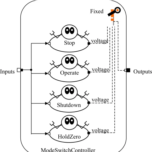
3.5.5 ModeSwitchController agent

The ModeSwitchController agent is given in the figure 3.7. It consists of four agents in fixed

priority coordination. The HoldZero agent is a controller agent with the lowest priority that

keeps the platform at its home position. The Shutdown agent becomes active when the STOP

button is pressed for four seconds. When active, it brings the translators of the linear motors to a

position where they are just above their lower end stops and then it shuts down the program and

switches off the power. When the START button is pressed, the Operate agent becomes active

and the manipulator is then in operation mode. Two parallel working agents perform the

operation mode, see figure 3.8. The PathFromFile agent reads the reference file samples into an

array and presents every sample time a value to the PID agent. For settings of the PID controller

see appendix D. The manipulator then performs the motion as specified in the sample file. In the

case that the starting point of the reference path is not the same as the home point of the

manipulator, the platform moves slowly to this starting point and then the motion is performed

according to the reference path. This functionality is integrated in the PathFromFile agent.

22

Fig. 3.7 Pool with agents of the ModeSwitchController

Fixed

ModeSwitchController

Stop

Operate

Inputs Outputs

voltage

voltage

Shutdown

HoldZero

voltage

voltage

When the STOP button is pressed, the Stop agent, which has the highest priority, becomes

active and stops the manipulator by bringing it back to its home position. The Stop agent pool is

given in figure 3.9. It consists of a Brake agent and a GoSteadyAll agent. The brake agent is a

speed control agent that brings the speed of the manipulator to zero. When the STOP button is

pressed, the momentary speed is determined. This measured speed is used to generate an inverse

desired speed step to zero. A low-pass filter filters this desired speed step and the output is the

reference for the speed controller. By using a filter, a smooth reference is generated without

much computational effort.

When the speed of the manipulator is almost zero, the Brake agent becomes inactive and the

GoSteadyAll agent becomes active. This agent brings the manipulator to its home position after

which the Stop agent becomes inactive. Like the Brake agent, also the GoSteadyAll agent works

with a low-pass filter. Now the a desired position step is filtered to create a smooth reference

path. After the home position is reached, the HoldZero agent automatically becomes active and

keeps the manipulator at its home position. The manipulator is then ready and waiting to go in

operation mode again.

Parallel

Operate

PathFromFile

PID

Inputs

Outputs

voltage

Fig. 3.8 The Operate agent pool.

Implementation of the safe controller system

23

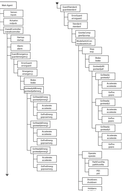
3.6 Total overview of the MAC system

In figure 3.10 an overview is given of the total MAC system in hierarchical form. With the aid

of IDITMAC created software can be compiled as an executable file to implement in the

computing system of the manipulator. Also a dll file can be created for simulation in 20-Sim. It

can be concluded that the agent based approach enables a convenient design process. The results

of the simulation and the implementation will be discussed in chapter 5. The code for the total

MAC system is given in appendix E.

Fixed

Stop

Brake

GoSteadyAll

Inputs

Outputs

voltage

voltage

24

Path generation

25

4 Path generation

4.1 Introduction

To perform motions with the manipulator, a motion profile input is needed by the PathFromFile

agent. Motion profiles vary in shape and order. In one-dimensional manipulators, the shape of

the motion profile is restricted to a straight line only, whereas in a multiple axes manipulator,

much more complex shapes can be defined. Usually, profiles are defined as piecewise

polynomials. The order of the profile gives the smoothness of the path. Higher order motion

profiles are easier to follow by the end-effector, but require more complex computation and

usually imply larger accelerations. This chapter will discuss path generation in general for

multidimensional manipulators and a generally applicable tool for path generation will be

developed.

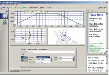
4.2 Tools for path specification

For performing a motion, the controller of the actuator needs a sample of the path at each

sample instant. This means that the path has to be presented to the controller as a list of

reference points. It is a laborious and error-prone job to create this list manually, especially for

complex trajectories. A tool on the market which allow us to give up begin points, end points,

speed, acceleration etc. and creates the reference position samples from these parameters, is the

Motion Assistant from National Instruments [www.ni.com/motion]. See figure 4.1 for a

screendump of the tool.

26

The Motion Assistant allows specifying motions in a graphical manner. By clicking and

dragging with the mouse, we can manipulate the shape of the motion. Types of shapes that are

available in the tool are straight-line movements and arc movements for up to 3 degrees of

freedom. For the order of the profile we have the option between second order and third order

profiles, which are also called respectively trapezoidal and s-curve profiles (these terms refer to

the shape of the speed curve). A major drawback of the Motion Assistant is that it works only

with hardware interfaces from National Instruments. This conflicts with the desire for a

generally applicable path specification tool. Therefore the Motion Assistant will not be used

further. Based on concepts as present in the Motion Assistant, the choice has been made to

develop a path generation tool, which is hardware independent. This will be discussed in the

next section.

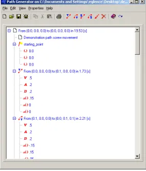
4.3 The Path Generator

The generally applicable tool, see figure 4.2, uses an XML format to store motion information in

an structural way. See Appendix C for an introduction to XML. The tool is written in Borland

C++ Builder. An advantage of this is that the programming environment allows us to work

directly with XML documents. This is done with the component TXMLDocument. It has

methods like AddChildNode, GetChildNode, GetNodeName for manipulating nodes in an XML

document directly.

Path generation

27

The tool creates reference points in three coordinates. For the Imotec manipulator these

coordinates are interpreted as positions x,y,z of the end-effector. The reference points are

transformed according the inverse kinematics of the manipulator. For the Imotec manipulator

this is done with [2-1]. At the moment no clicking and dragging options are available to set the

shape of the motion. Also checking the created path with a plot must be done externally. For

this, free plotting programs like GNUPLOT can be used. Motions are built up of segments. Each

segment is a motion from standstill to standstill. Segments with initial and final speed not equal

to zero are considered, but a problem with this is that discontinuities in speed and acceleration

will arise at the joint between two segments. This can be overcome by connecting the segments

with a spline movement or a Bezier curve. A major drawback of this is that considerable

computational effort is needed for control over the shape of the Bezier curve. The manipulator

could exceed its workspace if the Bezier curve is not well defined. So for the moment we only

consider motion segments from standstill to standstill.

Available motion shapes are straight line and arc shapes. The latter of course only in case of two

or more dimensional manipulators. Profile types that can be chosen are trapezoidal and s-curve.

It is desirable to have the opportunity to enter different values for the acceleration and the

deceleration of a single segment. This option is included in the Path Generator. See table 4.1 for

the functions of the Path Generator.

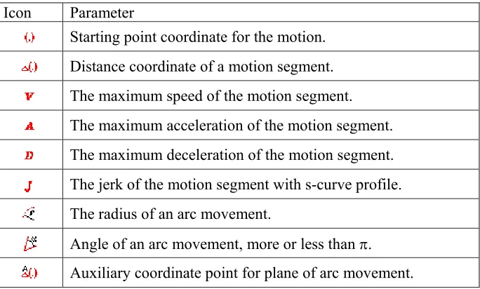
When the desired segments have been added, the parameters can be changed by double clicking

and editing the relevant items in the tree. The parameters and their meanings can be found in

table 4.2.

Button Function

Adds a straight motion segment with trapezoidal profile.

Adds an arc motion segment with trapezoidal profile.

Adds a straight motion segment with s-curve profile.

Adds an arc motion segment with s-curve profile.

Adds a wait in the motion

Deletes a wait or a motion segment.

Creates the file with reference samples

28

Icon Parameter

Starting point coordinate for the motion.

Distance coordinate of a motion segment.

The maximum speed of the motion segment.

The maximum acceleration of the motion segment.

The maximum deceleration of the motion segment.

The jerk of the motion segment with s-curve profile.

The radius of an arc movement.

Angle of an arc movement, more or less than

π

.

Auxiliary coordinate point for plane of arc movement.

After the desired motion has been set up, the reference sample file can be built by clicking the

button. The user will be prompted to enter the sample frequency of the controller system. A

sample file with extension .egl will be created. In the next sections, the algorithms for creating a

sample file from the XML file will be discussed. An example of a saved XML path file is given

in appendix C.

4.4 Trapezoidal

profile

algorithm

For creating a trapezoidal motion profile, the following parameters are needed. The maximum

speed

Vmax

that is allowed to be reached, the acceleration

A

, deceleration

D

and the length of the

stroke

h

. In figures 4.3 and 4.4 the position, speed and acceleration plots are given of the

trapezoidal motion for two cases: when the maximum speed is reached within the given stroke

h

and when not.

Table 4.2 Parameters of the Path Generator tool.

0 0.5 1 1.5 2 2.5 3 3.5 4 4.5

-0.2 0 0.2 0.4 0.6 0.8 1 1.2

pos speed acc

0 0.5 1 1.5 2 2.5 3 3.5 4 4.5

-0.2 0 0.2 0.4 0.6 0.8 1 1.2

pos speed acc

Fig. 4.3 Trapezoidal motion profile when

Path generation

29

In the algorithm, these two situations have to be distinguished. The algorithm is based on

integrating the profile of the speed to a position; the speed profile is obtained by applying the

given A and D. To take the right speed profile, a check must be performed to see if the

maximum speed can be reached within the given stroke

h

. This is done by calculating the

distance that would be travelled if the maximum speed would be just reached. If this distance,

which is called

h’,

is larger than the given stroke

h

, the maximum speed will not be reached.

With these tests, the following speed profiles are obtained and can be integrated, see figure 4.5.

To perform the actual integration, the times

Ta

till

Te

need to be known. These can be calculated.

First we take a look at the profile where the maximum speed is reached.

We introduce the times

T1

and

T2

which are respectively the times to reach

Vmax

with the given

acceleration

A

and to return from

Vmax

to zero speed with the given deceleration

D

.

max 1

max 2

V

T

A

V

T

D

=

=

[4-1]

with this the mentioned

h’

becomes.

1 2 max

(

)

'

2

T T V

h

=

+

[4-2]

The times

Ta

,

Tb

and

Tc

can be calculated as:

a 1

max

2

(

')

b

c

T

T

h h

T

V

T

T

=

−

=

=

[4-3]

For the situation where

Vmax

is not reached the following holds:

Fig. 4.5 Speed profiles that are integrated to a position profile.

0 0.1 0.2 0.3 0.4 0.5

Speed

Ta Tb Tc

0 0.5 1 1.5 2 2.5 3 3.5 4 4.5 0

0.1 0.2 0.3 0.4 0.5 0.6

Speed

30

2 2

2

d e

AT

DT

h

=

+

,

[4-4]

d e

D

T

T

A

=

[4-5]

This yields

2

2

2

D

D

A

h

=

+

T

[4-6]

Now the value of

Te

can be calculated as

2

2

e

h

T

D

D

A

=

+

[4-7]

With relation [4-5] also

Td

is known and the integration can be performed.

4.5 S-curve profile algorithm

For the s-curve profile, an extra parameter is needed in addition to the trapezoidal profile

parameters, namely the derivative of the acceleration/deceleration called jerk. For the

acceleration

A

and deceleration

D

the same value for the jerk is taken. Only the maximum

values of

A

and

D

can be different. Like the trapezoidal profile, also here there are several

situations that have to be distinguished. Now not only a check for reaching the maximum speed

has to be done, but also whether the maximum acceleration/deceleration can be reached within

the given stroke

h

. In figure 4.6 a plot of the S-curve profile is given when the maximum speed,

the maximum acceleration and the maximum deceleration are reached.

0 1 2 3 4 5 6

-0.5 0 0.5 1 1.5 2 2.5 3 3.5

pos speed acc

Path generation

31

The basis acceleration profile is given in figure 4.7. This can be integrated two times to obtain

the desired position profile. Before the integration can be performed, the times

Ta

till

Tg

have to

be known. If the maximum speed is not reached,

Td

equals zero. If the maximum acceleration or

deceleration is not reached, respectively

Tb

and

Tf

equal zero.

0 1 2 3 4 5 6

-0.6 -0.4 -0.2 0 0.2 0.4 0.6 0.8 1 1.2

Ta Tb Tc Td Te Tf Tg

First we distinguish whether or not the maximum speed is reached. The times

Ta

,

Tb

and

Tc

are

calculated to reach the maximum speed with the given maximum acceleration and jerk. Then the

times

Te

,

Tf

and

Tg

can be calculated to return from this maximum speed with the given

maximum deceleration and jerk. With the calculated times, the total covered distance

h’

can be

calculated. If this distance is smaller than the stroke

h

, it is certain that the maximum speed is

reached and

Td

is larger than zero. The time

Td

that the maximum speed holds on can be

calculated as:

max

'

d

h h

T

V

−

=

[4-8]

Then all the times are known and the integration can be performed. In the situation where the

distance

h’

is larger than

h

, it is certain that the maximum speed will not be reached. Then the

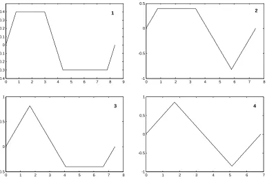
acceleration profile will have one of the four following shapes (figures 4.8).

32

Profile 4 is solved easily because of symmetry. Profile 1 can be solved in the following way.

First the distance

h’’

that is covered when the maximum acceleration is just reached is

calculated. This distance

h’’

is smaller then the stroke

h

. A formula can be derived for the

distance (

h

-

h’’

) that is needed to equal stroke

h

as a function of

∆Tb

. The order of

∆Tb

is two in

this function. That means that it can be solved with the ABC formula. Profile 2 and 3 are solved

on the same manner as with profile 1, also here a formula can be derived for the distance that is

needed to equal

h

as a function of

∆Te

. But here the order of

∆Te

is three in this function. This

means that there is no analytical general solution. The function can be solved numerically by

iteration. The formula’s for (

h

-

h’’

) are not given because of their large size and

non-transparancy.

4.6 Straight line movement

The straight line movement is a relatively simple movement. The trapezoidal or S-curve profile

that is generated has to be assigned to the straight line movement. If the manipulator is a single

axis manipulator then the transformation is not needed. For multiple axis manipulators like the

Imotec manipulator the transformation goes as follows. First the straight line movement has to

be decomposed in the distances along the dimensions, like

∆x

for the distance covered along the

x

-axis etc. Then the transformation becomes:

2 2 2

h

= ∆ + ∆ + ∆

x

y

z

[4-9]

0 1 2 3 4 5 6 7 8

-1 -0.5 0 0.5

2

0 1 2 3 4 5 6 7 8 9 -0.4

-0.3 -0.2 -0.1 0 0.1 0.2 0.3

0.4 ₁

0 1 2 3 4 5 6 7 8

-0.5 0 0.5 1

3

0 1 2 3 4 5 6 7

-1 -0.5 0 0.5 1

4

Path generation

33

x

x

pos

h

y

y

pos

h

z

z

pos

h

∆

=

∆

=

∆

=

[4-10]

With

pos

the instantaneous position value of the trapezoidal or S-curve profile.

4.7 Arc

movement

The arc movement is more complex to generate but also more difficult to enter/define by the

user. In

xy

-manipulators the parameters needed are a beginpoint, endpoint and the radius of the

arc. However this is not sufficient to define the arc motion unambiguously. Figure 4.9 shows the

possible arc motions with only the parameters above given.

0 0.5 1 1.5 2 2.5 3 3.5 4 0

0.5 1 1.5 2 2.5 3 3.5 4

Arc 1 Arc 2 Arc 3 Arc 4

R R

.

.

Beginpoint

Endpoint

From the figure can be seen that there are four possible arc movements: two arcs that make a

smaller angle than

π

and two arcs that make a larger angle than

π

. Defining that the arc motion

is clockwise from beginpoint to endpoint for the smaller angle arcs and counter clockwise for

the large angle arcs, makes the method more unambiguous. This means that in figure 4.9 only

arc 3 and 4 are possible. To complete the method also a choice between arc 3 and arc 4 has to be

made. This is done by entering an extra parameter, which defines whether the angle of the arc is

smaller or larger than

π

.

34

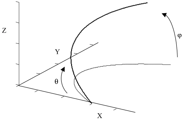
In three dimensional manipulators the arc is not restricted to the

xy

-plane. An extra parameter is

needed to define the plane of the arc. There are various ways of defining this plane. For

instance, an option is to first define the arc in the

xy

-plane as with two-dimensional

manipulators. Then by giving up two angles the arc can be placed in the desired plane. This is

what is done in the Motion Assistant from National Instruments, See figure 4.10.

X

Y

Z

ϕ

θ

A major drawback of this method is that the endpoint of the arc motion cannot be entered

directly by the user. This is highly desirable when defining a motion. A better method which

allows entrance of the endpoint is the following method. A third auxiliary point is entered which

defines the plane together with the begin and endpoint. The auxiliary point is given up with

respect to the beginpoint. This method is used in the developed Path Generator tool.

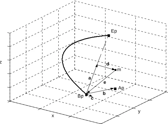
4.8 Assigning the sample reference points to the arc movement

To create the actual arc movement, the trapezoidal or S-curve profile has to be assigned to the

motions along the axes of the manipulator. In this section the procedure for a three dimensional

one like the Imotec manipulator will be discussed. A two dimensional transformation can be

derived easily from the three dimensional one. In figure 4.11, some vectors are defined that are

needed for the conversion. An arc movement can be described as the rotation of vector

e

in the

plane of the arc. This vector rotates from the beginpoint

Bp

to endpoint

Ep

, with a speed conform

the motion profile that is used (trapezoidal or S-curve).

Ap

is the auxiliary point of the arc

motion that defines the plane of the arc movement.

Path generation

35

.

.

.

Bp

Ep

a b c

d

Ap

.

e

z

y x

Ap

is entered as a point with respect to

Bp

and therefore equals vector

b

. The centre point

m

of

the arc has to be determined to create the rotation vector

e

. The point

m

can be found on the

following way. First the vector

a

is found as:

a

2

p p

E

−

B

=

[4-11]

The normal on the plane of the arc motion, vector

c

, is found by:

a

c b

= ×

[4-12]

We define a new vector

g

, which is aligned with

d

, but has not the same length as

d

.

a

g

= ×

c

[4-13]

Then the vector

d

can be found as

2 2

1

a

d<