7668-TM-2_New_Techniques_and_Equipment_for_Correlation_Computation_Dec1957.pdf

Copy Ir~)..

NEW TECHNIQUES AND EQUIPl-IENT FOR CORRELATION Cm.lPUTATION

Technica 1 l-lemorandum 7668-TM-2

James F. Kaiser and ,Roy K. Angell December 1957

Contract AI' ))(616)-)950 Task 50678

The research reported in this document was made possible through the support extended the Massachusetts Institute of Technology, Servomechanisms Laboratory, by the United States Air Force (Weapons Guidance Laboratory, Wright Air Development Center). under Contract No. AI' ))(616)-)950, M.I.T., Project No. D.S.R. 7668. It is published for technical information only and does not represent recommendations or conclusions of the sponsoring agency.

Approved

Servomechanisms laboratory

ABSTRACT

This memorandum, whioh is in two parts, desoribes some reoent developments in the design of correlation computers.

In the first part, the underlying theory of the correlation function and its calculation are summarize~ and the effects of finite averaging time, sampling, and quantization are discussed. Theoretioal analy~is, based on the work of Widrow, and experi-mental evidenoe are introduoed to show that for many a.pplioa-tions no significant change oocurs 1n the oorrelograms for quantization above 4 or 8 levels, oontrasting sharply with the previous praotice of specifying 100- to 200-1evel quantization. For certain applioations, even two-level quantization yields significant results. A classifioation of types of correlation computers is introduced and is followed by a detailed survey and description of the many components and circuits whioh may be used to perform the required mathematical, operations.. Using the oomponent survey as a basis, two oorrelator designs for a particular requirement - one analog and the other analog-digital - are outlined and discussed in detail. A comprehen-sive bibliography is inoluded~

The second part of the memorandum conoerns the design and

operation of a two-level real-time correlator. This correlator, whioh was construoted to experiment with two~level quantization, is designed around the ability of the magnetic,-o'ore shift regis" ter to acoept and store, in time sequence, information whioh has been given in the form of the binary digits ONE and ZERO. Inputs in analog form are sampled and quantized to two levels

(one bit) and 'inserted into a ten-'element shift register. Parallel outputs from all cores are multiplied by the output of the last oore, thus forming produots with different time displacements. The products are averaged ih low-pass filters, and the resulting ten-point correlogram is displayed continu-ously on an oscilloscope or with a voltmeter. ,The oorrelator was tested with periodic and random inputs,' and the evaluation

of the results indicates the practicalitiof t~o-level quanti-zation and the possibi.li:ties for real-time eleotronio

oorrelation.

ACKNOWLEDGMENT

In addition to the authors, other laboratory staff members who oontributed, through oonsultations or direot assistanoe, to the researoh reported in this dooument are Mr. Harry Pople, Mr. Douglas Ross, and Professor A. K. Susskind. Their help is gratefully aoknowledged. Mr. John E. Ward has served as editor for the completed dooumentw

FOREWORD

The material in this ~e~orandum is the result of two different studies made during 1957 in the Servomechanisms Laboratory. The material in Pa~t I is adapted from a study, "Correlation Computer Design Study," by J. F. Kaiser performed for the Communication Biophy'sics Group Of the Research Laboratory of Electronics, M.I~T. Funds for this work were provided by the Caspary Research Grant to M.I.T. Although this study was made for a particular corr~lation application (bio-electric poten-tials). the excellent summary of basic theory and techniques makes it valuable for any correlation problem. Those portions

of the study which are of g~neral interest have been adapted for use in this memor~ndum. and only the specific design

details of a correlator for the bio-electric application have been omitted. Perm'ission of Professo'r W. A. Rosenblith of the Research Laboratory of Electronics for use of this material is gratefully acknowledged.

The material in Part II is a stUdy performed as a Master's

Thesis by Mr. R. K.Angell and supported 'by the Air Force under Contract AF33(6l6)-3950. This thesis was a direct outgrowth of the study in Part I and was undertaken in order ,to demonstrate the practicality of a two-level real-tim~c6rrelator, sometimes referred to herein as a "one-bit correlato~"r The thesis was supervised by Mr. J~ F. Kaiser. The ,equipment was constructed solely to demonstrate the principle, and its sciccess indicates that two-level correlators of this type could be designed for many correlation problems and would have great advantages in

speed and complexity over existing methods.

This work has been supported as part of the airborne data-processing studies under Task 50678 of Contract AFJ3(6l6)-3950 because of the growing significance of oorrelation techniques in modern information processing. Correlation techniques are appearing in more and more of the literature concerning recon-naissance, intelligence, identif-ication ~nd location of unknown electromagnetic transmissions, and transmission of information at signal-to-noise levels much less than unity. The material

should be of interest ta anyone performing oorrelation analysis of data of any kind~

John E. Ward

TABLE OF CONTENTS ' " ' .

LIST OF FIGURES .12!.&!!. xiii

LIST OF TABLES

PART I

CONSIDERATIONS IN THE DESIGN O'F CORRELATION COMPVTERS

CHAPTER I

CHAPTER II

A. B. C. D.

E.

INTRODUCTION'

THEORETICAL ASPECTS OF CORRELATION ANALYSIS

THE CORRELAT*ON FUNCTIONS TIME SERIES CHARACTERISTICS

EFFECTS OF FINITE AVERAGING TIME, SAMPLING, AND IMPERFECT INTEGRATION ON ,T:a;E ACCURACY OF THE C,ORRELATION SPECTRUM ANALYSIS

. QUANTIZAT;ION AS, APPLIED' TO THE' .

COMPUTATION OF CORRELATION FUNCTIONS

1. Theoretical Consider~t1ons

~< •

2~ Experimenta~ Results

CHAPTER III STuDy OF BASIC SYSTEM TyPES FOR

CORRELATION CQMPUTATIONS

A. . INTRODUCTION

B. SYSTEM BREAKDOWN '

C. SYSTEM 'SPECIFICATION

D. BASIC SCHEMES FOR PERFORMING THE

OORRELATION COMPUTATION .

E. fD'XSCUSSIONOF POSSmLE SYSTEM DESIGNS

AS TO COMPONENTS

1. Delay System

2 .. Multipliers

3. Integra tor$ and Accumulat,ors

" ,\

.>:,;:.

4.

Division

5. Output Equ1pmemt

CHAPTER~V A. B. CO' DO'

APPENDIX

BIBL10GRAPHY

INTRODUCTION

CHAPTER

I A.

B.

D.

OHAPTER II

A. B.

O.

DO'

TABLE OJ' CONTENTS (continued)

RECOMMENDATIONS FOR A OORRELATOR

DESIGN

GENERAL RESULTS

AN ANALOG CORRELATOR.

AN ANALOG-DIGITAL OORRELATOR

COMPUTATION OJ' SPECTRA·

CORRELATION DETERMrNATIOH USING

FILTERS

' "

PART II

A TWO-LEVEL REAL-TJXB OORRBLATc)R

.E!.I.!

HJ:STORICAL

AND

THEORETICALBAOKGROtnID

CORRELATION FUNCTIONS

OOMPUTATION OF CORRELATION rUWOTIOKS

L

An Analog Correlator

2~ A

Digital Oorrelator

LDI:tTATIONS ON MEASUREMBIT

or

OORRELATION FUNCTIONS

1.

Continuous Oorrelator

2..

Continuous Averaging witb

an

Ideal Integrator

).. Oontinuous Averaging with a

Low Pass J'tlter

4~

Correlation on Sampled 'Inputs

E:rI'ECT$. OJ' SA.MPLDG AKDQ.UAtn'lZATXOK

. . . '

1..

Sampl :Lng

2.

Q.uant:Lzation

GENERAL DESlGN CONSlDERATIONS

THE MAGNETIO OORE, SHIn RIGISTBR

OPERATIONAL TIME SEQ,UlKCIS

SUMMATION

AND

AVBRAGING

DISPlAY

or

RESULTS

CHAPTER III A. B. C. D. E.

CHAPTER IV

A.

B •.

TABLE or OONTENTS (continued)

DESCRIPTION OF ODWUITS

MAGNETIC1 CORE SHII'TREGISTER SHIFT PULS'E GENERATOR

SAMPL].NG ¢:::1!RCUIT OUTPUT CIRCUITS DISPLAY G,IRCU,IT

TESTS AND CONCLUSIONS

CORRELOGRAMS OF PBRIODIC FUNCTI:ONS CORRELOGRAMS OF RANDOM FUNCTIONS

1. White No~se

2. Band-limited Noise

C. COMMENTS ON POSSIBLE CJ:RCU.IT

IMPROVEMENTS

D. CONCLUSIONS

APPENDIX I DERIVATION OF INPUT-OUTPUT

RELATIONSHIPS FOR TWO BASIC. INTEGRATORS

A. MILLER INTEGRATOR

B. BOOTSTRAP INTEGRATOR

APPENDIX II A DERIVATION FOR THE IMPULSE

RESPONSE OF THE COUNTING RATE: METER

APPENDIX III A DIODE MATRlX SWITCHING C mCUIT

APPENDIX IV CALCULATION OF AUTOCORRELATION

FUNCTION OF BAND LDIITEDNOISE.

APPENDIX V CORRELATIONS OF TWO LEVEL NOISE

1 2

3

5

6

7 8 9 10 11 12

13

14

15

16

17

18

19

20 21 22

23

24

25

26

LIST OF FIGURES FOR PART I Variation in the Autooorrelation as a Result of Time Varying Statistios Variation in the Autooorrelation as a Result of Time Varying Statistios

RMS Computation Error as a Funotion of kecord Length·

Qu~ntization Box Size vs. Correlation

Coefficient of Quant1zer Input Signal with Correlati6n of Quantization Noise as a Parameter

Probability Distribution Funotion of Quantization Noise

Amplitude Distributions Not Satisfying the "Nyquist Condition"

Correlogram, Run B Corre1ogram, Run B

Power Density$peotra, Run B Corre1ogram, Run A

Correlogram, Run A

Power Density Spectra, Run A

Changes Made .in the Amplitude Distribution to Study the Effeots of Bias, Amp1ifioation Faotor, and Saturation

Corre1ogram,

3

Levels, Run A Correlogram,

7

Levels, Run B

Power Density Speotra, 3 Levels ,·Run B Correlation Computation Blook Diagram Two-Bit Multiplier

Digita1-Anaiog Multiplier

Output Equipment for Digital Computation Output Equipm~at £or Analog Oomputation Analog-Digital C~nverter

Analog Correlator

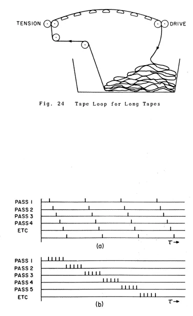
Tape Loop forr Long Tapes Data Spacing Sohemes Drum Head Control

21 "28 A-I 1-1 2-1 2-2 20.13 2-4

2-5

3-1

3-2

3-3

3 ... 4

3-5

3-6 4-1 4-2 4-3

4-4

4-5

A-I A-2 A-3 A-4

LIST OF FIGURES ,OR PART

r

(continued) Digital-Analog Oorrelator

Head .Stagger Scheme

Possible Filter Scheme t,o Aid in Oorrelation Determinati.on

LIST OJ' I'mURES )'OR PART :n: Measurement Errors of Low Pass RC filter ;

Idealized Magnetic Oore and :Its Hysteresis Loop

Two Stages of' a Single Line Shift Register Time Sequence Flow Chart

Basic Integrator Forms

Counting Rate Meter Oircuit

Correlator Block Diagram (Autocorrelation

Arrangement) . ,

Shift Register Oonnections and Waveforms· Shift Pulse Generator

,Sampling Circuit

Output Oircuit (One Channel) Waveforms for Sinu~oidal Input Oorre1ograms of Sinusoidal Inputs Correlogram Fluctuations

Test Equipment Arrangement.and Filter Characteristics

Amplifier Gain Effects on Oor.reloc~ams.of Noise Inputs

Ef'fects of' Sampling Rate on Oorrelograma of' Band Limited Noise

·Low-Pass j'ilter

Counting Rate Meter Ou.tput Voltage Waveform Blook Diagram of D~ode Matr1xSwitohlng System Power Spectrum of White Noise Passed Through an Ideal Band-Pass Filter

I

I I I I I

LIST ·OJ' TABLES

Properties of Some Basic-Analog Multiplication Schemes

Elements Required in Diode Matrix Multiplier Accumulator Size aa Affeoted by Bit Size and Number of Samples

xv

43

48

PART I

CONSIDERATIONS IN THE DESIGN 01' OORRBLArTJ:ON OOMPUTERS

by

CHAPTER I INTRODUCTION

This study of schemes for realizing the correlation

computation was undertaken to review the present state of the art of computation, both analog and digital, and to review the theory of the basic correlation computation as a statisti-cal tool with the intended goal of arriving at the oorrelation computer design which will best suit the requirements of its users. The most important design oonsiderations are speed and acouracy of computation, versatility and reliability of its operation, and the economy of construction and operation. In short, what is desired is the fastest, most accurate, simple, and reliable corr~lation oomputer.

In choosing a method for correlation computation, it is apparent that the choice must depend heavily upon the fo~ of the input data, the form desired of the output data, and the time scale of the data--considerations which arise in the use of the machine. To permit the most flexibility in' the choice of a design or method of computation, we have, chosen to separate the

overall problem into two parts. The fir~t part concerns that of properly applying the correlation oomputer to a data reduc-tion task. Considerations are those of accuracy and those of the choice of the length of data to be oorrelated and the num-ber and time separation of the computed correlation values. The second part concerns the design of acorrelator which will perform the single oorrelation oomputation as' rapidly

al8

possible.

This study is arranged into three s'ections. The first section deals with the theoretical concepts of correlation. The effects of finite averaging time, sampling, quantization, and averaging method are discussed. Spectral analysis is also considered. In the second section, the discussion centers on the various schemes used for correlation computation with

.4

CHAPTER II

THEORETICAL ASPECTS OF CORRELATION ANALYSIS A. THE CORRELATION FUNCTIONS

The oorrelation funotions that provide the basis for the analysis of random, ,time funotions are defined (15)* as

+T

CP12(T) = lim

-

1

S

_{f l (t)f2 (t+T)dt}

1'-00 2T _-T

(orossoorrelation)

+T

CPll (T)

=

lim

..L

S

fl(t)fl(t+T)dt

T-oo 2T

-T

(autooorrelation)

If fl(t) and f 2 (t) are integrable square (whioh ,is almost always met in praotical si tua tiona), then CP12 (T) an? CPll (T) are defined for all T and pos'sess Fourier transform's that are

oommonly oalled power-density spectra. These speotra are

respectively

00

<P

12 ( w )

=

2ln

S

-00

<Pll (w)

=-1-

_2n

00

S

CPll(T) COSWT dT

-00

(comple~

'cross-power-dens~ty spectrum)

(power-density spectrum)

In using correlation techniques. sorIle, investigators prefer to base their analysis on il1'terpretatioil of the relevant

corre-lation functions, while others prefer Lnterpre~ation of the

speotral funotions. Disregarding for the moment the relative

merits of each metho.d, the literature appears to be in general

agreeme,nt that oomputation oC speetra is most readily

aooom-plished ,from the oorrelation t'>b1l'11ctiions rather than from the ·da:t.adi>reortd.y.Wi til this opini.on as a basis, we shall now

:oronsideir t:heoomputational probll. ... _ that exi.st in the practioal oa!J:culla:t!Lon o,f ttlbe'co'rre la t i 011 :iiUf'lc t i«i)ns •

* Number in paren'theses refe,rs {t.o .numbered items' in , t he Biblio~raphy.

6

The integral expressions fot' the correlation functions are seen to be based on a time averagew This requires that the time function being oorrelated must be one generated from a sta-tionary process, 1. e., a process whose st,atd.stioal. eha,racteris-tios are time invariant. If the time function is not station-ary, interpretation of the correlation funct~on in its simple form beoomes difficult if not impossible.,

The correlation integration 1s oarried out over limits tending toward infinity_ Thus, information over all time is required of the time function.. Practically, this is impossible; and one must be satisfied with analysis of a finite amount of data. The questions which arise are what is the effect of a finite averaging time and what is the effect of using an imper-fect in'tegrator to perform theintegratton operation?

Because of the availability of high-speed digital oomput-ing machines, the investigatbr must be acquainted with the problems and effects of the sampling and quantizati:on opera-tions onth.tim~ functions, these operations heini tequired on the data for digital computations.

This section will treat these probl~ms in sufficient

detail to' give the investigator Some idea of the ma·gnitude and type of er~or in~roduced by each.

BO' TIME SERIES CHARACTERISTICS

The use of the time average in the calculation of the <I '

7 is chosen, much longer oomputation time is required: and it is necessary to interpret the effects of averaging the different levels of variation. On the other hand, if short correlations are taken, a view of how the correlation changes with level of variation is obtained at the sacrifice of slightly higher

varianoe of error.

Provided the length of record of the short runs is at least an order of magnitude (~actor of ten) greater than the period of the lowest frequency or time constant of th. process other than those corresponding to changes in level of variation, then the average oorrelation for the process may be obtained by simply adding and averaging the short-time oorrelations. This seoond method of looking at several short-time correlations has several important advantages over computation of one long-time correlation. First, it gives one more of a feel for the

effects of change in activity on the correlationw Second, it may result in important savings in computation .t~me if it is

shown early that the short term oorrelationsdiffer only

slightly from one another. This factor is ~xtremely important from an economic point of view since it is desi~able to obtain as much interpretable information as possible from a unit of computation time.

In support of the ideas just discussed, reference is made to Figs. 1 and 2, which show two common types of correlogram

(oorrelation function) characteristics.* In e~bh figure the correlogram at the top was obtained from a 60-second run length. The second and third correlograms oorrespond to computation

over the first 7-1/2 seconds and the last 7/12 seconds, respec-tively. The change in correlogram characteristics with time is most obvious. For example, in Fig. lc the apparent modulation

*

These partioular data, which were obtained from physical experiments on cell potential activity in the human body, are

used because they are typical of the data to be correlated in many applications and also because' they were readily

RECORD

LENGTH-0.7

T - SECONDS

(a)

(b)

(e)

RECORD lENGTH-7.5 SEC. FIRST EIGHTH

(a)

(b)

(e) .

RECORD

LENGTH-7.5 SEC.

FIRST EIGHTH

Figs. 1 and 2 _{Variation in the Autocorrelation as a Result of}

9

of the periodic component is missing whereas both Figs. la and lb show this phenomenon clearly. Likewise, from Figs. 2a, 2b, and 2c, the first 7-1/2 seconds of data gives a much more varia-ble oorrelogram than does the last 7-1/2 seconds of data. The last 7-1/2 seconds of data, however, gives a correlogram having much the same features as the long 60-second oorrelation.

These examples point out clearly the advantages to be gained in short-term oorrelation and what sacrifices are made to obtain them ..

One source of error in oorrelation that results from non-stationary series is oaused by drift or very slow change in the value of the mean of the signal. This slow variation oan be removed by coupling the signal to the oorrelator through a high-pass RO filter. The break frequency of this filter is chosen to be lower than the lowest frequency of i.nterest in the oorre-lation by at least a faot'or of two. FilteI:'s of identical

charaoteristics should be used in each of the .two input chan-nels to the correlator.

0_ EFFEOTS OF FINITE AVERAGING TIME, SAMPLING, AND IMPERFEOT INTEGRATION ON THE AOOURACY OF THE CORRELATION

The accuracy of the oorrelation computation depends on the averaging time interval, the number and spacing of samples if sampling techniques are used, and the charaoteristics of the integrator or averaging device. Much material has appeared in the literature discussing in detail the first three items (14, 15, 16, 17, 19. 20, 21, 24)~ Of these r~ferences. (20) gives perhaps the most complete and readable dis~ussion of these effects.

10

preoise oorrelation f ... notion for the prooess but also of ~he

tourth'-order probability den~ity distr~buti.on. Hence,exaot

determination of rms error oan be made for onJ.y the simplest theoretical cases.

If one assumes a fixed data length, oalculation of the oorrelation function by t.he use of saQ1ple~ and summation

results in a higher value of rms error than if the computation were done oontinuously.. This is easy to understand i·f one

looks upon the sampling operation as discarding some ot the information in the data. The rms oomputation error for the sampled case varies inversely al3. the number of samples for deterministio signals and .inverselyas the square root ot the number of samples for the rand,om,signals. These variations are approximate; exact oalculation of error again requires'kn~wl­ edge of both the seoond- and. fourth-order ·probability·(iistribu-tions of the input data •

. If the integrati.,?n required in the corr·el.at1on· computation 'is ,·to be accompli'shed ·a~'ProximatelY-.by the ·u·se of a filter,

then in general a longer .reoord. length is required for tli~ same

, ' .' acouracy of computation.

We can therefore o'Ottolude (neglecting '1.na6oura.otes .... ·tn. the components) that for

a

specified acouracy .of' correlation compu-(' tatton the speed a·t which th~ oomputat:bonoanbe oarried out is . direct ly dependent on the speed at whioh t·he data can enter the I

.

.

oomputation. For a fixed da~a speed t the oontinuou's-type

correlator utilizing a pure ;lntegli'ator giv:e~ t.he most acourate result.

Because calculation of the varianoe requ'ires knowledge at

11 The autooorrelation funotion of suoh a signal is given by

=

where CT 2

=

mean square value of the signal

W₁

=

bandwidth of the signal in rad/seo

T ~ oorrelation time shift

If we denote by L the reoord length, then the expression for

2

the varianoe CT <p of the oorrelation determination as a funo-tion of T and L beoomes

CT 2

=

CT

q? {

-2w T }

I

+

e 1 (I +2W₁ T )

In the oases of interest to us

Henoe, the varianoe becomes approximately

2

"q>

For very small T shifts

whereas for large

2

4

"

= ....a.-<p WI)..

or

T

or

~=

2

CT

shifts,

!.!e

2

"

WIT >

I

=

ii>lL

12

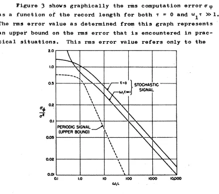
Figure :3 S~01liS graphically the rms computation error (J' cp as a fUnotion of the record length for both T

=

0 and W₁T »1.

The ~ms error value as determined fro~ this graph represents an uppe~ bound on the rms error that is encountered in

prac-tical situations. This rms error value refers only to the

Fig. 3

tt;

ttl

2.0..---.---..---....---.---.

1.0 1---1~ ... --4_----+---~~--~ 0.5 I__--~\--"

...

-~-r _tao

1

_STOCHASTIC

w,t-J

SIGNAL

0.2 0.1 0.05

\

\

\ \

\

~---+-~\.--~~~~~--~I---~

\ \

\

,

\

\

PERIODIC SIGNAL ~

(UPPER BOUND) \

1---4---~\----~~~~----.~

\

\

\

\ \

0.02 1__---4----+_~\-4----+-~...lio,,-.I

\

\ \

~Ol~--~ _ _ _ _ ~ _ _ _L~ _ _ ~~--.-~

0.1 1.0 10 100 1000 10.000

RIS Computation Error as a Function of Record Length

calculation of single points on the correlation curve. From knowledge of this error value, little can be inf~rred about how the shape or overall characteristics of the correlation curve for a finite record l~ngth deviate from tbe true co·rre1ation characteristic. As'" t'ule, the fit will be closer than that

indicated by the value

or

the variance.

For periodic signals the variance diminishes with the square of the record length. For example. if the signal is assumed to have the form

f (t )

=

A cos ( w t

+

e)

The variance of ~t as a function of r8oor4 length b~comes

thus

but

whence

rr 2 CP

rr

CPmax

.!.L

CPmax

=

=

=

=

4

2

!.-.

(.S.in W.L)

8 wL

I

sin, w L

WL

sinw.L

J2

wL

1)

Thus, for

wL

=

nn, where n is an integer

rO,

the variance

is equal to zero. As an upper bound·to the rms error we use

I

sin w L

I

₀

<:

_{wL <} :!!.

J2

wL 2

.!L

:::

CPmax ,1 _:!!.

< wL

J2

wL 2

A plot of this function is shown in Fig.). Thus, for example,

a record length of only

5

periods of .the frequency w can result

in a 2 .. 2% rms computation error, in t'he cOr're1a1;iion coefficient

as an upper rms limit. If we recall the correlat,ion function

of Fig. lc where a very pronounced periodloityof approximately

w

=

63

radians/seo is present, it is easy to understand in one

sense why the obtained oorrelation is so smooth. Lw for this

oase is

460

corr-esponding to a rms error of O.l!J,~ if the periodic component 1.s assumed to. be the only component of importance.

One must be very oareful in applying the results of these two simple oases to praotical situations primarily because the prooesses usually enoountered are nonstationary and of wide

variability in statistical makeup. The two cases are presented

only to sarYe as a broad guide.

To give an example of how the results might be misleading,

refer again to Figs. 1a and lb. There appears to be a marked

component. This oould be oharaoteri.zed by two signals of

nearly equal frequenoies beating with one another. The

expression for such a signal oomponent oould be written as

f 1 ( t)

=

cos w_{1 t (l} + a cos W 2 t .)

or

where _{WI »W 2} O' In such a case tt oan· be shown that the

value of the varianoe of the comput~d oorrelation funotion ts

mostly dependent on the low frequenoy w_{2 of the modulatton ..}

If the nodulation is of very low frequ·enoy, extremely long reoord lengths must be used to reduoe the' theoretioal variance

to a tolerable value.. W~ know from ex·perienoe that extremely_

long reoords are not required to show the presence of the modu-lation; yet from oaloulation of the'varianoe a10ne, we may be

seri.ously i.n error with only moderate record lengths. From

the experienoe gained by different members of, the Servomechan-isms Laboratory, the rule-of-thumb criterioJ:J that the reoord

length should be· at least 8 to 10 time.s the maxtmum time shift

has been found to give very satisfaotory ,resultsr

If sampling techniques are used, the same rule' appltes

. " . .

.

to reoord length with the additional requirement that the

number of samples be at :Least 10' and preferably greater than

4

.

10 for good correlation results

(3,

8, l5~~

D. SPECTRUM ANALYSIS

'Although the general or main oharaoteristios of the autocorrelation funotion appear, to be affeoted, only slightly by the use of finite records of moderate length, ,the fact that errors or variability are present should oaution the investigator in trying to read too muoh out of small

irregu-larities in the correlation function. We feel that there is

1.5

is studied. The'spectral study would not be intended to

replace the cOit'relogram study. but 'instead • 'to augment it

and thus add gre~te~ insight into the problem.

Investigators using spectral graphs (18, 20, 22, 23) bave

found that the numerical computation of the spectra from the

. }.

computed autocorrelation function can be carried out in general easier and faster than by the use of schemes involving band pass fi,ltering and averaging of the original time function. This is especially true when use is made of special purpose

anal'og

or

digital computers. Thus.' the computation of spectra

would follow logically t'he pre,sent computation of aut()correla-tion funcaut()correla-tions.,

The spe,ctra, as are the functions fr'om which they are

obtained,' are affeoted by the use ot a'finite record length.

. . . . . 1 , .

The most important effect is that of limiting the frequency

\f I . . . I . ~

resolution to a minimum possible value wr,es of

=

(Reference 18)

L

where L is the record length and 'T " ;~, the maximum time

, max

shift of the correlation function. This resolution is seldom

ach;i,.eved . in practical cases because of ,th,e excessive amount of ,.",

calQulation required.. In the more usual situation, the number

" ,

of.~omputed points of the spectral function is made equal to

the number of computed values ot the correlation

function--usually' in t;he range of fifty to two hunt;lredpoints. In .this

case, the maximum frequency resolu~ion obtainable in the

spect.it'um, is equal to the reciprocal of the maximum time shi:Ct

of, the correlation function.. To realize ttiis resolution, a

special weigbting function (23) 1s introduced in the

trans-format,ion_computation in order to reduce the e:Cfects of trun-cation of the correlation function. _. The introduction of the {,

s~ecial we1ghtil)g function adds litt.le ,.to, the complexity of

'.

the Fourier trans:Cormation computation. The e:Cfects of the

addition of th~s weightirlg function on the obtained spectral

16

An example of the use of spectra in the correlation

studies will be polnted 'Out in the next section where- the

effects of quantization are considered in some detailr

E... QUANTIZATION AS APPLIED TO THE COMPUTATION 01' CORRELATIOII

J'UNCTJ:ONS

lw

Theoretlcal Considerattons

If 1t is first assumed that the data to be correlated i.

in a continuous analog 'form, then in 'order to perlorm tbe

oor-relation computation digitally the data must first be sampled

at discrete evenly spaoed potnts and then the magnitude of tbe

sample digitized or'quan:tfzed. Theeffeots of samp1inc

bay.

already been disoussed..

The problem remains as to wt..at

efeeots does quantization introduce..

It would bea.dvantaseous

to know. how ooarse1y one is

permi~ted

to quantize the data

without introduoing exc'essive errors 1n the correl.t,ton

oompu-tation..

:If a' special-purpose digital maohine 1s to be

~uilt

to perform the computation, lt 1s known that the size and

oa.-plezity decrease and the .speed increases as the si&e(bit

length) of the input number is 1l'educed..

:i:t 1s then to one's

advantage to use as smail a number (as coarse a quantization)

as 1s toleraMe in view of the errors introduced ..

The theoretical study of the effects of q,uanti&ation

carried out by Widrow

(24,)

suggest that extremely ooarse

q.u·aD-tization is perm1ss1b1e in the correlation

oomp~tation

with

the resultant

stat~stica1

errors being calculable., I'or silDp1e

first .. order pr'Ocesses. it 1s shown that the noise 1ntroduoed

b,y

q,uantization is oomp1etely uncorrelated with the

stati8t~o8

ot the process i.t a oertain relation exist s between the

quan-tisation coarseness and the oharaoteristio funotion of tbe

amplitude distribution of the input.

If the relation is

satis-fied. then the moments of all orders of' the unq,uanti.ed 81pals

are oalculable from the moments of the quanti.ed 8igna1 and

inf"ormation on tbe q,Uantization coarseness.

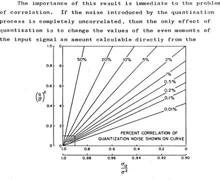
correlation of the quantizer input signal witb itself. For signals with Gaussian distributed amplitudes. Widrow (24)

gives the following relation that approximates olosely the correlation of quantization noise as a function of the correlation ooefficient of the quantizer input signal:

wbere

2 2 ( 0"12) -411 0" 2 1-

2

=

e q 0" 0"

N

=

normalized oorrelation of quantization noise with signal

0" = standard deviation of quantizer input signal q

=

quantization box width

0"

12

=

normalized correlation coefficient of the

quantizer input signal

17

A plot of this relation for different values of the correlation of quantized noise is shown in Fig. 4. The use of this figure

18

as

follows. If

a

bo~ size or quantization coarseness of say q

=

20" ts used, then one can, by reading off the

tnter-section of the slanting lines with the ordinates dete:rmined

2

by (')

=

4,

obtain the correlation value of quantization noise to be expected for any normalized co~relation ooeff~cient of the signal being quant ized. Thus. we see tha t 'lor q

=

2 0"

(extremely coarse quantization) the noise introduced by quan-tization is less than

1%

correlated with the signal for all correlation ooefficient of the signal less thari 0.1 in

magnitude.-Van Vleck* (68) has shown that :for two-level quantization the correlation functionR(T) of the quantized signal is simply related to tbe correlation function cp(T) of the continuous signal as

R ( 'T )

=

£

s~n

.

-1

'IT

Thus, in the two-level case :for correlation values less than

0.54,

R('t) is within

5%

of cP(,.).

18

The importance of this result is immediate to the problem of correlation. If the noise introduced by the quantization proces~ is completely uncorrelated, then the only effect of quantization is to change the values of the even moments of the input signal an amount ca1culable directly from the

1.0 0 , - - - y - - - r - - - , . - - - . , - - - - " " 7 I

0.8 8

0.6 6 0.4 4

0.2 2

PERCENT c;ORRELATION OF QUANTIZATION NOISE SHOWN ON CURVE

o

o~-~-~---~---~---~----~

1.0 0.8 0.6 0.4 0.2 0

1.0 0.98 0.96 0.94 . 0.92 . 0.90

Fig. 4 Quantization Box Size VS. C~rrelation Coefficient of

Quantizer Input Signal with Correlation.· of Quantization Noise as a Parameter

quantization size. All other obtained points on the correlation curve (i. e., other than at ,.

=

0) are theoret iccl?1ly unaffected by the quantization, a very inte·resting· and' useful result. A series of experimental tests, that will be mentioned suqse-quently, were carried out which verified this theoretical result quite well.

The errors ~n the even moments of the correlation for T 0

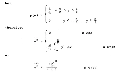
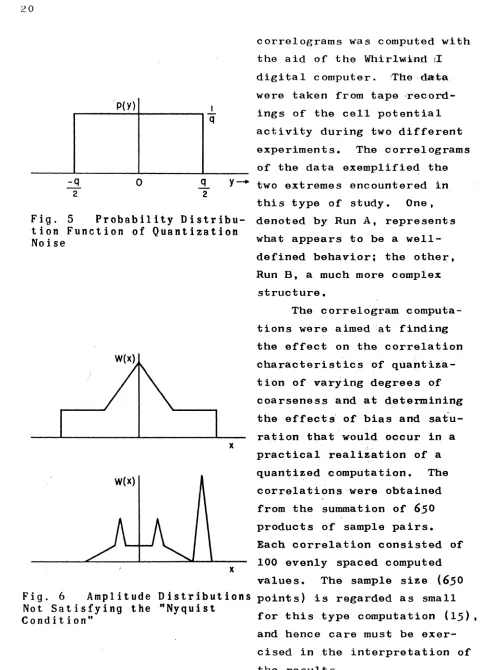
of the quantized signal are found simply by considering the flat-topped distribution of the quantization noise. This dis-tributi.on is shown in Fig.

5.

The moments are given by

n

y

=

00

S

yn p(y)dy

19

but

{:

9.- _{< y <} S.

2 2

p{y}

=

Y <

-

a

y > 9..

2

,

2

therefore

0 n odd

n

=

9.

Y

52

6

n

dy

y n even

q

0

or

n (9.) 2

n

y

=

n even

n + 1

Thus, the mean square and mean fourth values of the noise are, respectively

2

Y

4'

y

=

=

2

L

12

4-

9-80

It must be recalled that these theoretical results assume that the distribution of amplitudes of the input signal or signals satisfies the "Nyquist Condition" with respect to quantization size~ Signals whose distributions are Gaussian or very nearly Gaussian satisfy this oonditionapproiXimately up to extremely ooarse quantizationr Fortunately, most of the data from the physioal prooesses of nature.have amplitude distributions that are. approximately Gaussian. The distribu-tions which can oause serious errors when quantization is introduced are those possessing discontinuities or large changes in slope. Fig.

6

gives several examples of these types of amplitude distributions.

2~ Experimental Results

20

" P(y)

-q

o

2 2

,

q

correlograms was computed with the aid of the Whirlwind i1 digital computer. 'The . data.

were taken from tape -record-ings of the cell potential activity during two different experiments. The correlograms of the data exemplifie~ the

y-. two extremes encountered in this type of study. One,

Fig.

5

Probability Distribu-

denoted by Run A, represents

tion Function of Quantization

Noise

what appears to be a

well-W(x)

w(x)

Fig. 6

Amplitude

Not Satisfying the

Condition"

x

defined behavior; the other, Run B, a much more complex

structure.

The corre1ogram computa-tions were aimed at finding the effect on the correlation characteristics of quaritiza-tion of varying degrees of coarseness and at determining

the effect~ of bias and

satu-ration that would occur in a prac,tica1, realization of a quantized computation. The corre1ations'were obtained ,from the summation of 650

products of sample pairs. Each correlation consisted of 100 evenly spaced computed values. The sample size (650

Distributions

points) is regarded as small

"Nyquist

'

x

21 The first graph.

rig.

7,

shows,thd etfebt of quantization coarseness on the corre1atipn characteristics of the Run B data. It is seen that quantization to

:3

bits

(8

levels)

results in only minor amplitude differences with no apparent changes in overall oharacteristios. For 2-bit

(4

levels) quantization, the variati.ons in amplitude deviation are some-what greater but still the general characteristios are retained. For the extreme oa~e of one-bit (2 levels) quantization ooarse-ness, Fig. 8 shows that only the major oharaoteristios of cor-relation are intaot. The theoretical results of the previous section indicate that better oorrelation should be obtained. The disorepancy between theory and experiment in this situation

is believed to be due p;rimarily to the small sample size.

Aside from this, the results of one-bit quantization are quite startling and interesting.

The comparison between correlations was made on the

general basis of how olose1ythe curves conform to one another .. An additional o~eck into the effects of th~ quantization is made by observing the power density spectra, of the

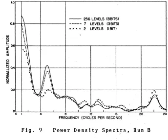
correla-tions.· As shown in Fig. 9, quantization'down to three bits introduces no deteotable ohanges in the frequency

character-,

istics of the spectra .. The minima and maxima, appear unchanged frequency-wise. One-bit quantization appears t6reduoe the frequency definition as notable differences are present,

especially at the ~igher frequencies. This, again, is believed due to the sm~ll ~am~le size~

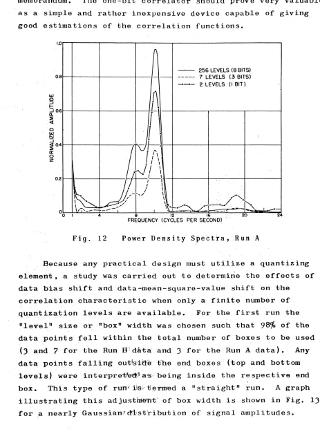
The data of Run A was subjeoted to the ,salDe prooedure as outlined above. Q,uantization was a,djusted to be 8 bit s,

:3

bits, 2 bits, and one bit, respectively. The results are show" th Figs. 10 through 12 ..

It is immediateiy _. ( , appa~·nt . .bai the same general

22

12

8

-4

12

8

4>11 (Z')

4

-3

Figs. 7 and 8

QUANTIZATION - - 256 LEVELS (8 BITS) • • • • 8 LEVELS (3 8ITS) 0000 4 LEVELS (2 BITS)

QUANTIZATION

2 LEVELS (I Brh.

23

by coarseness of quantization. The only perceptible effect in the spectr~study was that in the one-bit case the dis-crepancies were large primarily at the high frequencies. In all cases, the relative magnitudes of the two adjacent maxima at 8 and 10 cps were preserved.

~ ~

.0,-,----...,.----,---,

- - 256 LEVELS (88ITS)'

0.8 --- 7 LEVELS (3 BITS)

k k W W 2 LEVELS (t BIT)

:::;0.&

0-~

<[

o

I&J

~Q4~~-H--+_J\----~----+_---~---~---~

-J <[

~

~

Q2~r---·~~_T~---~----_+---~~---+_7_or--~ k •

°OZ~I~-~4-~~-8~-~-~12~-~-~16-~~~~-~~

FREQUENCY (CYCLES PER SECOND)

Fig. 9 Power Density Spect!a, Run B

From the similarity of' results obtained f'rpm these tests on two sets of data of quite different correlation character-istics, it can be concluded that very sat1sfact~ry correlations can be computed digitally using quantiza~ion as coarse as

8

levels

(3

bits). Quantization to

4

levels (2 bits) appears to give good results and there is every indication that this result should improve if' the sample size is increased to a moderate value.

Because quant.izatt.ion to 2 levels (one bit) gives a

24

16

12

8

4

4»11 (t)

0 0

-4

-8

-12

16

12

8 4 . " (f) 0

0

-4 -8

-12

w_

"

0 0

0

0.2

Figs. 10 and 11

QUANTI ZATION

- - 256 LEVELS (8 BITS) • • • • 8 LEVELS (3 BITS)

0000 4 LEVELS (2 BITS)

QUANTIZATION

2 LEVELS ( , BIT)

25

memorandum. The one-bit correlator should prove very valuable as a simple and rather inexpensive device capable of giving good estimations of the correlation functions.

I&J

o

1.0

0,8

~

~0.6

,~ ,<I

o

~

::J

~0.4

a::

o z

0.2

{\,

- ' - 256 LEVELS (8 BITS)

, - --- 7 LEVELS (3 BITS)

-.--

2 LEVELS (I BIT)

1\

-1-\

{ I

I

-I-i

!

,

It,

I \

• I \

flU

AI

_{" ,}

,

I I

,

_I

t

/'/r'

t · ,

""',

\ . , v"/ \

' J

"i'-\ ~",/

.

.,..., ... _/.,=~~

'"

1"\

"-'_-- ....

-.--~

~'I"

'", I

...-4 8 12 16 20 24

FREQUENCY (CYCLES PER SECOND)

Fig. 12 Power Density Spectra,RunA

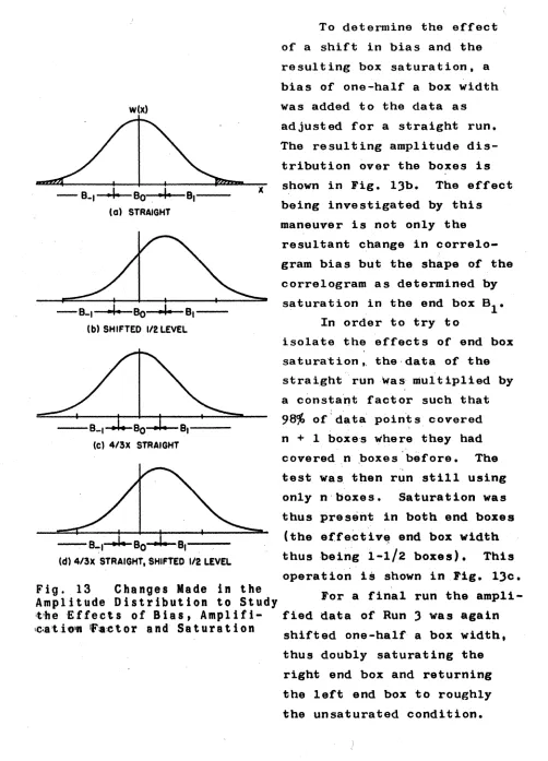
Because any practical design must utilize a quantizing element, a study was carried out to determi~e the effects of data bias shift and data-mean-square-val~e shift on the

cor~elation characteristic when only a finite number of

quantization levels are available. For the first run the "level" size or "box" width was chosen such that 98% of the data points fell within the total number of boxes to be used

(3 and 7 for the Run g'd.ta and 3 for the Run A data). Any data points falling out~s'itle' tihe end boxes' (top and bottom

lev.els) were interpre~~jl a;;g; being inside the respective end box. This type of run" :iJ!:F-tj:ermed a "st ra ight" run. A graph

26

wbO

- B . I ,I-Bo .•

1.

B I -(al STRAIGHT

-8..1 ..

I.

BO

.1.

B I -(bl SHIFTED 112 LEVEL

(el 4/3x STRAIGHT

(d) 4/3x STRAIGHT, SHIFTED 1/2 LEVEL

lC

To determine the effect of a shift in bias and the resulting box saturation, a bias of one-half a box width was added to the data as adjusted for a straight run. The resulting amplitude

dis-tribution over the boxes is shown in Fig. l)b. The effect being investigated by this maneuver is not only the

resultant change in corre10-_{. , .} gram bias but the shape of the corre1ogram as determined by saturation in the end box B1 •

In order to try to

isolate the effects of end box satura·tion ,. the· data of the straight· run was· multiplied by a c~nsta~t factor such that 98% of: d·a tapoirit s covered _{. ,}

.

n + 1 boxe·s ~llere they had cover$d ." .boxes· before. The

..

test Wa~ then run still using only n·b6xes. Saturation was thus pres~~t in both end boxes

(the effeotive, end box width thus being 1~1/2 boxes). This operation is shown in Fig. 1)0.

Fig •. 13

Changes Made in the

.

Amplitude Distribution to Study

For a final run the

ampli-.t'he£·ffects of Bias, Amplifi-

fied data of Run) was again ,c;a'tio'll IF,a·.ct

or a nd Sa t u ra t ion

_{shifted one-half a box width.}

27

This manipulation is shown in Fig. 13d. using 3 levels for the quantizationw

Figure 13 was prepared

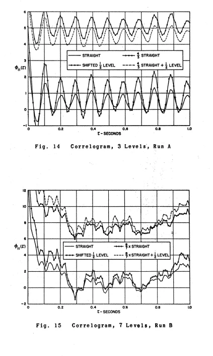
Figure 14 illustrates the correlations obtained by

applying the sequence of four manipulations to the Run A data. The first observation is that the general character, including

the envelope modulation, of the correlation is retained

throughout all the operations. At only three levels of quan-tization this result is very rewarding because it indicates that the bias and saturation effects are not extreme at all .. The shift in correlation level for the second and fourth runs was approximately the value computed from the square of the bias set in. If the data had an initial mean value of f, then it can easily be shown that the change in correlation value

- --2

for an added bias b is simply 2fb + b

It is noticed that the effect of saturating the end boxes as in Run 3 gave a wider variation in the correlogram. This" was to be expected since the end boxes are now being used mo~e

than in the first run. Despite the heavy ~aturation effect in the right end box for Run 4, the general correlation character-istic was quite well preserved. In all oases,the major

frequenoy information remained fixed in the spectrum.

The same sequence of operations was applied to the Run B data first with quantization at ? levels and then at 3 levels. The correlograms of Run B at

7

levels, Fig. 15, strongly

support all the oonclusions reached on the 3-1evel Run A results. At 7 levels the differentcorrel,ations ~emarkably

display all the mode~ate and major rises and falls of straight correlation. Amplifying the data as in r'uns three and four again results in a slightly increased correlation amplitude due to greater use of the end boxes.

The correlograms of Run B at 3 levels showed much

increased variability over that at

7

levels.- ror this r~asop, a power spectrum presentation of the results is chosen.

Fig.

16

shows these results in detail. It should first be mentioned. that the amplitude scale factor for runs ,two and

28

6

,

fi

'~

I

~

I

I:

,

\ f

!

.\ r

~

r

,

1\

.. \ F

,

I

\V/

\\t' \V,:

,

,

\\ti' 'Vi'

'

,

, I _\

\VJ'"

,

~I

\V,I

\yr

,V/

'

,

,

,

_\

'

I , \ I , I \ I , I

,

'

\ I \

,

\

,

, ' r \ I, \ I I, I

\ I

\

,

\ I

\/

IJ \../ I...J

\ I \ /

\ l

'

:

v

,

... ,

..

4

-STRAIGHT -tSTRAIGHT

"

- SHIFTED

i

LEVEL

r--~'

---- t

STRAIGHT +

i

LEVEL

II.

A

II.

h

/'

I

f

'/'

f

r

f\,

Ai

\

l'

I"

f

o

I/V

1

I

rr

VI

I

\.A't

\ I

I

J

~.J

\

,

~

J

'if

..

'(j

~

" y 'VI v

H

I

o 0.2 0.4 0.'

0.'

1.0

t-SECONDS

Fig. 14 Correlogram, 3 Levels', Run A

12n-~~----~--~----~--~----~----~--~----~--~

<1>11 (t) - 'X STRAIGHT

4 r---rr--+~-f+H ----'XSTRAIGHT+iLEVELH--P~

-2~--~----~--~----~~~----~----~--~----~--~ _{o 0.2}

0.4 0:6 0.8 1.0

t-SECONDS

The first general comment is that the power density

spectra have roughly the same general shapes. For runs 2,

), and

4

the spectra are noticeably different from run 1

in regards to location of peaks and valleys in the range

of frequencies from

7

cps to 11 cps. The maxima at 5 cps

I . o r - , . - - - - , - - - , - - - ,

LLl

o

~

i2

0.8

:E 0.6

<t

fa

N

::i

~ 0.4

cr

o z

0.2

- - STRAIGHT SHIFTED ~ LEVEL

~)( STRAIGHT

~ )( STRAIGHT SHIFTED

i

LEVEL

~

-L-J--t_-~::=r~~~~~:.:~~~~:~~~~~~~~~

o

~~----o I 8 12 16

FREQUENCY (CYCLES PER SECOND)

Fig. 16 Power Density Spectta,

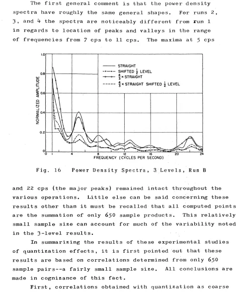
3

Levels, Run B

and 22 cps (the major peaks) remained intact throughout the

various operations. Little else can be said concerning these

results other than it must be recalled that all computed points

are the summation of only 650 sample products. This relatively

small sample size can account for much of the variability noted in the )-level results.

In summarizing the results of these experimental studies of quantization effects, it is first pointed 'out that these

results are based on correlations determined fr~m only 650

sample pairs--a fairly small sample size. All conclusions are

made in cognizance of this fact.

First, correlations obtained with quantization as coarse

as 7 levels () bits) were excellent when compared with both the

analog results and the 256-level results. There are no

I.,

)0

as a result of this quantization. A chQnge in bias or scale factor of

'!7%

(1/2 level) produoes no noticeable or uncomputa ... ble change in the oorrelat ions. frequency inf'orma tion again being unaffected. The cl1.ange in mean-square value due to quantization is oomputable and 1s relatively small fot' the 7-level case. As a whole. the 7-level study supports the theoretical results rather closely. It is recalled that the normalized value of the correlation functions were usually considerably less than 0.5. especially in the case of the Run B data.

Second, the quantizations at

4

levels (2 bits) produced

"""

correlations whose variability although large oould possibly be acceptable in lieu of the fact that this variability could partially, at least, be attributable to the small sample size~.

Again frequency information appeared to be unaffeoted by bia$ shifts and saturation effects.

The results of one-bit quantization were sat~sfactory enough to merit additional study in tbe form o:('a thesis

CHAPTER III

STUDY OF BASIC SYSTEM TYPES FOR CORRELATION COMPUTATION A. INTRODUCTION

This section begins with a discuSSion of the dependenoe of correlator type on the input and desired output information. The various schemes availabLe fo~ realizing each correlator

type are discussed as to their advantages and disadvantages. The section closes with a rather oomprehensive listing of most

of the currently used techniques (that are applicable) for

performing the operations of delay and storage, multiplication, integration, and recording~

B. SYSTEM BREAKDOWN

The procedure of obtaining the correlation function of a set of' data involves three basic steps. The first step oon-sist s of transforming the data into a fot"Dl .that. the correlator can use. If automatic analog or digital computers are to be used, the data must be transcribed to the form ·that each computer can interpret and operate upon. 'rhe second step

consists of performing the correlation computat.ion. The third and final step is the transformation of the computer results to a form suitable for interpretation or other use.. This form may be a pl~tted curve, a tabular listing, a scqpe plot, a

~unched tape, etc.

The choice of a device to perform the actual correla-tion computacorrela-tion then is seen to depend upon both the form.of the input data and on the desired form of the output results. The form and character of the input data impose the more

stringent restrictions on the type of correlator than does the output requirement. The restrictions in design due to these specifications are d~scussed in detail in the pertinent sec-t ions 1ihich follow .•

32

c.

SYSTEM SPECIFICATION

For the purposes of disQussaon it will be assumed thattb~

oorrelator is to be used as an investigative tool fo~ tQG

analysis o£experimental, da"''' "ti'om physioal prooesses..

4

di£fi ... culty, then, that is encoun'&ered is that the i.nvestigator often does not know what part of the oorrelation funotion or what part of the power speotrum contains the i.nforrnation he is seeking. He. is theref'ore in a sense forced to look at the oorrelation funo-tion in rather fine detail over a si ... able range in. time delay. This unoertainty and wide variation requires that the

oorre-lator be designed suoh that the spaoing between oomputed values and the number of oomputed.yalues oan be var:Led over wide

,limits. It is not unoommon. for a oorrelation to oont,ain

~P'Ward,s of, one hundred oomputed point s. The' spaoing sbould be

o~osen

so that there

'a~e

at

l~ast

four

od~puted'Pb!nts

per the

. , ' , '

higl;1.est f,requenoy to be discerned in the d~ta .. ', Nyquist t s sampling theorem requires an absol'ute min'iDlu~

or

tw'o po:l.nts per oyole. On this basi~ the ,'total numb'er:'of, o.oQlPutedr.ro1nts should be equal to the product of the ratio of the higbest

frequenoy to lowest frequenoy of inter~stand,the'number of

points per oyol* of the highes~ £requ~ncy.

To make possible a time soal.e 'Change; _{, ,} th~ test data can be recorded on magnetio tape.. This permits the 1nv9stigator to use more efficiently the correlatj:'on oomputer by' 'all'owing him to run the data i.n as fast 'as the oomputer oan prooess it.. A frequenoy modulation soheme is usually usedJnthe recording to enable the low frequein91es:to be recorded:. and to help

prevent loss of information during subsequent re-'recor.ding and playbaok.

For purposes of disoussion, the form desired of the output of the correlator is assumed to be a point-by-point plot of the oorrelation funotion. As will be pointed out later, it may also be advantageous if the output is also reoorded in a form that will easily permit fUrther oomputation by'a general ..

33

With the input and output specifications thus spelled out literally. it is desired to determine the correlation computer which will perform the single correlation computation as

rapidly as possible. The design is to have the versatility, and flexibility previously mentioned. and must be as simple and reliable as possible while retaining a computational acou-racy commensurate with data length and data statistics as outlined in Chapter II.

D. BASIC'SCHEMES FOR PERFORMING THE CORRELATION COMPUTATION To the writer I s knowledge. there are four principal t'ypes of correlation oomputers. The olassification is made on the basis of the mathematical manner in which the correlation coefficient is computed.

The first type is essentially the straight analog correla-tion oomputer. Its operation is as follows. A, value of t1m. delay 'T is chosen and fixed.. The data is then continuousiy

multiplied by itself shifted in time by T. The continuous

product is then continuously integrated. After a fixed length of time T the computation is stopped, and tlie'correlation

coefficient value is read as the analog of the flnal value of the integratorp The next point is comput~d using the same data but a different value of T~ Descriptions of sev~ral successful correlators of this type are found in referenoe,s l. 6. 'i, 9. '10. 11. 12. 13. 26.

The second type of calculation schem,e consists of a slight modification of the first type", In this 'system instead of com-puting the correlation on a point-by-point basis, the value of time ,shift T is slowly and continuously. varied. Thus, the

correlation function is generated continuously. In this scheme a very long data length is required. For the correlation to be meaningful, the statistics of the data must be reasonably time

The third type of correlation scheme is based on the sampling prit:'ciple. The data is sampled at a rate such that the adjacent samples oan be assumed to have statistics inde-pendent of one another. The sampling interval thus chosen is then greater than the maximum time shift of interest.. The ,correlation coefficient is then built up by summing a fixed

number of products of the sample of the time function and the sample of the time function shifted by 'T units of time. The

number of' .samples required for a fairly stable correlation function result has been discussed in Chapter II and is usually in excess of several thousand. Thus, this scheme requires a record length at least several thousand times the maximum 'T

shift. Correlators of this type are discussed in

(3)

and (8), and find their greatest use where the input information is

located in a high frequ~ncy pass band and whe~e ,avery long record length is available.

The fourth 'type consists of a slight variation of the third type, and is aimed toward a more efficient use of the record length. In this scheme the data is sampled at in~ervals

corresponding to the minimum time shift increment. '

Independ-enc~ of adjac,ent samples is not assumed or required.. Aga;Ln the

computation consists simply of a summation of afix~d number of products of samples. This scheme is usually employed when the computation is performed on a general-purpose digital computer. The record length required by this scheme is nearly

~

times

that required by the third type where N denotes the number of computed points.

E., }}ISCUSS:LON 01' POSSIBLE SYSTEM DESIGNS AS TO COMPONENTS The type-one system is essentially a continuousana10g computing system whereas the type-four system is basically a discrete computing system being most likely digital in fo~.

al though di.s-crete analog

sy-stem~" ~~e

possible. Because the basic correlation computation consists of four fundamental mathematical operations and because these operations can eaoh be accomplished by many oomponents, the possible numb~r of correlator designs is very great., The designs may involve entirely analog components' or all digital components, or may be a hybrid type utilizing both analog and digital techn1ques.

It is necessary to make a few general comments first before discussing the systems and components in detail., It is assumed first that the input to the correlator is to be data recorded on magnetic tape in frequency modulated form,. Because of bandwidth limitations in the recording scheme, the highest frequency component'of the input data is limited to

5

kilocycles per second for a JO-ip~t~pe sp~ed. Thus, a goal of the correlator design must be a capability of processing input data at this maximum Nite. For an analog system this specification sets the bandwidths r~quired of the individual computing components. For a ciigital system this specification partly establishes the minimum sampling and

computation rate. The other factors which affect the sampling rate are the record length and desired minimum spacing between computed correlation values.

Regardless of the sampltng rate, any ,type-four system will not be considered satis£actory unless it 'oan perform about' on an equal basis with the type-one system. Performance is

36

/

A-second ~oint to be brought, out is th~t both type-one an~

type-four correlators oompute the valu~s of the correlation

fUnction at discrete points., ;Because the input data rate :i.s assumed to be limited not by the computation process but by the data recording or storage means the time to compute one point on' the oorrelation function is about the same for both systems. If total oomputation time i$ to be reduced by computer design,

simultaneous computation of several points must be done. This

is termed multiplexing. One oonsideration therefore in

ohoos-ing a design must be based on how simply the sohoos-ingle point

oomputation method may be multiplexed. The total computation

time oan be reduced using this means by a factor of N where N

is the number of s:imultaneously oomputed' points.

,

In discussing analog type elements, attention must be paid to the problems of accuraoy, bandwidth, drift, and dependency

on tube characteristics.. For digital elemen:ts there is

essen-tially no drift problem, but attention must be 'directed n()w,to ,6omple.xityas a function of the bit size of the dat;;l numbers

and to the time required to per,form the particu;J,ar digital

operations.. It should also be recalled that theinpLJt 'data is

essentially 'of analog fo,rm.. The desired output ,1s ~n analog

plot and possibly a digital tabulation if ,sp~ctra are to be

caloUlated later. Thus, if digital means are:tobe used, both

analog-to-digital and digita1":,,to-analog oonverters,would be required.

As an ai4 tn evaluating and disoussing the different _,. systems, two data runs typical of the near extremes that a

correlator for the data discussed in Chapt'er II might encounter

are considered. These typioa1 runs are:

Highest frequency Maximum time shift Reoord length

Number of points desired

A

Sample rate for 5,000 sample s min.

. " CO;Mf,UTER, T,I;ME

Mal .T,iPte, 1.1>0 :,1, ,Speed .\!P 10: 1, ,Spread up

50 cps 5,000 cps 500 cps

1. sec 0 .. 01 sec 0.1 sec

10 Sec 0 .. 1 sec 1 seo

200 200 200

5 m sec 500 slsec

.05 m sec

50,000

slsec

Ji

10,0,:1, Sp.ee,d UP ,10 :,1 Speedup,

COMPUTER TIME; ,

Long, Run ,Real, Time,

Highest frequency 50 cps

Ma~im~m time shi.ft 2 se(!

Record length 2,000 sec

Number of points desir~d 400

A

5

m sec

Sample rate for 5,000 2"'1/2 s/sec samples min.

5.000 aps

.02 sec 20 sec

400 .. 05 m sec

250 slsec

500 ops

.2 sec

200

sec

400, .'

., m seo

25 slsee

The important oonstderations :lil:Dplied by these ru~s

are:

(1)

For

very short runs the sampl:Lng rate may have

to exceed the ioeciprocalo£ the m1ntmum time

shift

AT

in order to obtain a sufficient number

of samples 0'

(2)

If

a fix