Imaging and Control of Engineered Cells using Magnetic Fields

(1)

Imaging and Control of

Engineered Cells using

Magnetic Fields

Thesis by

Pradeep Ramesh

In Partial Fulfillment of the Requirements for the degree of Doctor of Philosophy

in Bioengineering

CALIFORNIA INSTITUTE OF TECHNOLOGY Pasadena, California

2019

(2)

(3)

ACKNOWLEDGEMENTS

“The truth is rarely pure and never simple. Modern life would be very tedious if it were either…”

Oscar Wilde

In the summer of 2017, a group of us went white-water rafting on the American river near Sacramento, CA. Since 2016 was a particularly strong El Niño year, the river banks were bursting at their seams and the rapids were at their strongest in nearly 7 years. Being an adventurous lot, we naturally chose one of the toughest runs and spent the day rafting down the river, experiencing our share of tumbles, flops, and the occasional boulder along the way. We emerged sopping wet, grinning and laughing about our collective fumbles, while basking in that feeling of having conquered a challenge.

As cliché as it sounds, that trip is a good analogy for this PhD, now approaching 7 years in the making. I am forever grateful to my thesis advisor, Dr. Mikhail G. Shapiro, who has been the proverbial raft along this journey. Thank you for your trust and faith that you placed in me when you asked me to join you in starting your lab at Caltech. Thank you for an inspiring problem, which proved to be a fascinating puzzle to work out. Thank you for giving me a richly adorned scientific playground, full of toys that kept me busy. Thank you for your generous support and burning the midnight oil with me when I was stuck. Finally, thank you for your sunny optimism and humor, which made the lab a fun place to learn.

(4)

Geoff Blake, Dr. Paul H. Oyala, Dr. Andres Collazo, and Dr. Alasdair McDowall for scientific advice, as well as opening up your respective labs for my experiments. Thank you to Dr. Rob Phillips and Dr. David Baltimore for serving as my undergraduate thesis advisors, as well as serving on my graduate thesis committee. Thank you, Rob and David, for having taught me to do bottom-up science and to always calculate before jumping into the melee.

Thank you to Hunter C. Davis and Marjorie Buss who have been such willing partners and enablers throughout our shared scientific adventures. I could only plumb such great intellectual depths with your support, and I hope to have such genial collaborators in the future. Thank you to Dan I. Piraner and Mohamad Abedi for being such good sports and joining me on so many of my impromptu adventures. A Hindu, a Muslim, and a Jew sounds like the perfect setup for a joke, and that is precisely what our office was. Thank you to Di Wu for having created such a fun and carefree environment. Thank you to Dr. George J. Lu and Dr. David Maresca, who have been such genial friends and mentors, and for patiently working through ideas with me. Thank you to Arash Farhadi and Anupama Lakshmanan for all the laughs, and to the rest of the Shapiro Lab for one of the most memorable experiences of my lifetime.

(5)

ABSTRACT

Making cells magnetic is a long-standing goal of synthetic biology, aiming to enable the separation of cells from complex biological samples and their non-invasive visualization in vivo

using Magnetic Resonance Imaging (MRI). Previous efforts towards this goal, focused on engineering cells to biomineralize superparamagnetic or ferromagnetic iron oxides, have largely been unsuccessful due to the stringent required chemical conditions. In this thesis, we introduce an alternative approach to making cells magnetic, focusing on biochemically maximizing cellular paramagnetism. Here, we show that a novel genetic construct combining the functions of ferroxidation and iron-chelation enables engineered bacteria to accumulate iron in

‘ultraparamagnetic’ macromolecular complexes, which subsequently allows for these cells to be

trapped using strong magnetic field gradients and imaged using MRI in vitro and in vivo. We characterize the properties of these cells and complexes using magnetometry, an array of spectroscopic techniques, biochemical assays, and computational modeling to elucidate the unique mechanisms and implications of this ‘ultraparamagnetic’ concept.

(6)

(7)

PUBLISHED CONTENT AND CONTRIBUTIONS

Ramesh, P.†_{Buss, M.} †_{et. al. (2019)}_{. “Remote Control of Cellular Localization in the G.I.}

Tract Assisted by Magnetic Particles.” In preparation. († _{Equal contribution)}

P.R. conceived the study. P.R. and M.B. designed the experiments, as well as collected and analyzed the resulting data. P.R. conducted the in silico studies on magnetic capture. P.R., M.B., and M.G.S prepared the manuscript.

Ramesh, P. et al. (2018). “Ultraparamagnetic Cells Formed through Intracellular Oxidation

and Chelation of Paramagnetic Iron”. In: Angewandte Chemie Internation Edition 57, pp.

12385-12389. doi: 10.1002/anei.201805042

P.R. conceived, planned, and conducted experiments, analyzed the resulting data, and prepared the manuscript.

Davis, H. †_{, Ramesh, P.} †_{et al. (2018).}_“_{Mapping the microscale origins of MRI contrast} with sub-cellular NV magnetometry”. In: Nature Communications 9, 131. doi:

10.1038/s41467-017-02471-7 (†_{Equal contribution)}

P.R. and H.D. co-conceived and planned the study. P.R. assisted in building the magneto-microscope and preparing the in vitro and in vivo specimens. H.D. acquired and processed the NV data, and conducted the in silico studies on relaxation. P.R. and H.D. performed the MRI measurements and analyzed the resulting data. P.R. also participated in the preparation of the manuscript.

Mukherjee, A, Davis, H.C, Ramesh, P. et al. (2017). “Biomolecular MRI reporters:

evolution of new mechanisms”. In: Progress in Nuclear Magnetic Resonance Spectroscopy,

(8)

LIST OF TABLES AND ILLUSTRATIONS

Number Page

Tables

T1 Measured and Theoretically Available Magnetic Susceptibility ... 39

T2 Culture media used in experiments ... 57

T3 Table of NV wavefunctions ... 116

Figures 1.1 Susceptibility spectrum ... 5

1.2 Chemical Exchange Saturation Transfer (CEST) ... 13

2.1 Ultraparamagnetic gene circuit ... 29

2.2 UPMAG cells are strongly paramagnetic ... 31

2.3 UPMAG cells can be magnetically captured ... 32

2.4 UPMAG cells produce enhanced MRI contrast ... 34

2.5 UPMAG cells can be magnetically isolated from ex vivo specimens ... 36

2.6 FLPM6A forms a ferrogel ... 38

2.7 Mössbauer Spectroscopy of UPMAG E. coli at 80K ... 41

2.8 Shift and Splitting of nuclear levels of 57_{Fe in Mössbauer spectroscopy... 42}

2.9 Idealized powder EPR spectra of paramagnetic species ... 45

2.10 X-band EPR of HSF, FLPM6A, and Fe(III) ... 46

2.11 Fit to EPR spectra of FLPM6A ... 46

2.12 CEST spectroscopy ... 48

2.13 Monte Carlo simulations of relaxation by UPMAG cells ... 50

2.14 Growth curves ... 51

2.15 Magnetic separation from complex mixtures ... 51

2.16 Gel chromatography of FLPM6A ... 52

2.17 DLS spectroscopy ... 53

2.18 Iron source ... 53

2.19 CD spectroscopy... 54

2.20 TEM images of FLPM6A ... 55

3.1 Concept of Cellular Localization Assisted by Magnetic Particles ... 76

3.2 In vitro model of the mouse GI tract ... 77

3.3 Simulated 2D field of the external magnet used for CLAMP ... 79

3.4 Simulated 2D field and field gradients in the in vitro setup ... 80

3.5 Magnetic properties of micromagnets used for CLAMP ... 81

3.6 Monte Carlo simulations of micromagnet capture in vitro ... 83

3.7 In vitro efficacy of CLAMP ... 85

3.8 In vitro capture of magnetized E. coli using CLAMP ... 87

3.9 Optimization of the animal protocol for CLAMP ... 89

3.10 Representative in vivo CLAMP results ... 91

3.11 Brightfield images of micromagnet displacement in an ex vivo specimen ... 92

3.12 Efficacy of CLAMP in vivo... 93

(11)

3.14 Representative ex vivo MRI on mouse GI tracts ... 95

3.15 Kinetics of large micromagnets in vivo ... 96

3.16 Brightfield images of micromagnet displacement ex vivo ... 97

4.1 Comparison of various magnetometers ... 112

4.2 Physical structure of the NV center ... 114

4.3 Characteristics of the NV center ... 118

4.4 Sensing techniques and protocols for NV magnetometry ... 119

4.5 DC vector magnetometry with bulk NV diamonds... 121

5.1 Subcellular mapping of magnetic fields in cells labeled for MRI ... 130

5.2 Predicted and experimental MRI behavior in cells ... 132

5.3 Magnetometry of histological samples ... 134

5.4 Dynamic magnetic microscopy in live mammalian cells ... 135

5.5 Simulated dipole fields ... 142

5.6 SQUID magnetometry and saturation of IONs ... 143

5.7 Additional cells for Monte Carlo library ... 143

5.8 Additional tissue sections ... 144

5.9 Additional live cells ... 144

5.10 Live cell imaging with extended time course ... 145

5.11 In silico models of T2 relaxation ... 146

(12)

NOMENCLATURE

Symbol Definition Units (SI) Value

𝐁 Magnetic flux density T Commonly referred to as the magnetic field

𝐇 Magnetic field strength A m⁄ Magnetic field produced by ‘free’

currents

𝐌 (Volume) Magnetization A m⁄ Magnetic dipole moment per unit volume

𝐌_𝐬 Saturation Magnetization A m⁄ Bulk magnetite ~ 4.46 × 105 𝐌_𝟎 Initial or remnant

magnetization A m⁄ material in the absence of a field Volume magnetization of the

𝐦 Magnetic dipole moment A ∙ m2

𝒎_𝒑 Proton rest-mass kg 1.67 × 10−27

𝒎_𝒆 Electron rest-mass kg 9.11 × 10−31

𝝁_𝟎 Permeability of free space H m⁄ 4𝜋 × 10−7

𝒆 Electric charge C 1.60 × 10−19

𝝌 Volume magnetic

susceptibility Dimensionless By convention, 𝜒 =

M H 𝜸𝑰,𝒆 Gyromagnetic ratio MHz T⁄ 𝛾𝐼: Nuclear gyromagnetic ratio

𝛾_𝑒: Electron gyromagnetic ratio

N Particle density m−3

𝒌𝑩 Boltzmann constant J K⁄ 1.38 × 10−23

Z Atomic number Dimensionless

𝒈_𝑰,𝒆 Landé g factor Dimensionless 𝑔_𝑒 ~ − 2.00 𝑔_𝐼 ~ 5.59 𝑻_𝟏, 𝑻_𝟐 Relaxation times s

𝑻_𝑬, 𝑻_𝑹 MRI pulse-sequence parameters

s

D Apparent diffusion

coefficient of nuclei in MRI m

2_⁄_s

𝜼 Dynamic viscosity Pa ∙ s 𝜂𝑤𝑎𝑡𝑒𝑟 ≈ 10−3

𝝁𝑩 Bohr magneton J T⁄ 9.27 × 10−24

J Total angular momentum

operator kg (m

2_{∙ s)} ⁄

ℏ Planck’s constant J s⁄ 1.05 × 10−34

S Total electron spin

operator J s⁄ ℏ√𝑆(𝑆 + 1)

(13)

𝝐_{𝒊,𝒋,𝒌} Lattice strain constant 1 s⁄ Electric-field coupling constant for an NV-axis. Typical values are of order GHz.

𝑨_𝒉𝒇 Hyperfine coupling

(14)

C h a p t e r 1

NON-INVASIVE BIOLOGICAL IMAGING USING MRI

1.1 Motivations

“When scientists develop methods to help them see things that were once invisible, research always takes a great leap forward.” Nobel Prize Committee in 2008

The development of genetically encoded optical reporters has revolutionized the study of cell-biology by directly coupling changes in optical contrast to the expression and activity of molecular targets within the cell. Despite the technological advances in optical imaging, however, all optical contrast agents are fundamentally limited in their utility for studying cell-biology in vivo

in opaque animals. This is primarily because the amplitude of electromagnetic radiation in the visible (and near infra-red) spectrum is rapidly attenuated (I ~ e−z_{) due to photon scattering and}

absorption by tissue.1_{Consequently, fundamental questions in mammalian biology pertaining to} animal development, neuroscience, and immunology for example, remain unanswered because of our inability to observe cellular biology in vivo.

On the other hand, magnetic fields can permeate through the body unencumbered – a feature which arises from the fact that tissue only weakly interacts with magnetic fields. Magnetic Resonance Imaging (MRI) scanners therefore exploit these subtle interactions to form 3D anatomical images of living animals in a safe manner, without the use of ionizing radiation such as X-rays (CT) or γ-rays (PET).2_{However, there are at present few sensitive and genetically} encoded reporter genes for MRI – a fundamental technological bottleneck that limits its utility for studying cell and tissue biology in vivo.2_{Among the most sensitive and widely used contrast} agents in MRI, superparamagnetic iron oxide nanoparticles (SPIONs) act by shifting the local magnetic susceptibility of an MRI voxel (~ 1 mm3_{) by several parts per million (ppm);}

consequently, voxels that contain SPIONs, as well as their nearest neighbors, appear darker relative to background in T2 weighted MRI. While SPIONs have enabled successful cell-tracking

(15)

or studying biology within dividing cells.3_{If magnetic nanoparticles could be genetically} encoded and biomineralized, they would arguably remove one of the largest barriers to the widespread use of MRI for studying cell biology in large, living animals. Lastly, such genetically encoded magnetic nanoparticles would also enable remote control of biological function using magnetic fields.

However, despite extensive efforts by the MRI and synthetic biology community, there has been scant progress in engineering a biosynthetic pathway that is truly capable of biomineralizing superparamagnetic iron oxides in model cells (gut microbes, mammalian cells) of interest to human health. Faced with these hurdles, we set out to develop an alternative approach to making

cells magnetic. Although our ‘ultraparamagnetic’ cells are less magnetic than naturally

magnetotactic microbes, their strong paramagnetism is sufficient to enable more sensitive detection in vivo using MRI, and magnetic capture ex vivo using strong magnetic field gradients. In this thesis, I will first cover the physical principles of MRI and how they broadly inspired our efforts to engineer ultraparamagnetic cells. I will then extend the concepts learned through our cellular engineering efforts to highlight a new method for localizing magnetized therapeutic cells in the GI tract noninvasively. Lastly, again motivated by our efforts to engineer paramagnetic cells, I will introduce a new modality for optical magnetic field imaging, which we used to experimentally study the microscopic origins of MRI contrast.

1.2 Physical principles of Magnetic Resonance Imaging (MRI)

(16)

∆𝐸 = 𝑚_𝑠ℏ𝛾_𝐼𝐁_𝟎=ℏ𝛾𝐼

2 𝐁𝟎 (1.1)

Within any MRI voxel at any given time, there is an excess of nuclear spins (𝐌_𝟎= 𝑁_𝑉𝛍) that are aligned with the magnetic field of the MRI scanner (𝐁𝟎 𝑘̂), as described by the Boltzmann

distribution (Eq. 1.2a).

𝑁_aligned

𝑁_{anti−aligned} = 𝑒∆𝐸 𝑘𝐵𝑇⁄ (1.2a)

However, the Zeeman coupling between the nuclear magnetization (𝐌_𝟎) and 𝐁_𝟎 is weak when compared with thermal energy, and therefore results in a spin polarization of approximately a few parts per million (Eq. 1.2b) under ambient conditions in typical field strengths (20 ℃, 7 T).

𝑁_aligned 𝑁anti−aligned~ 𝑒

3.9×10−6

→ 3.9 ppm H 11 polarization (1.2b)

In addition to creating a population imbalance, 𝐁_𝟎 also exerts a torque on 𝐌_𝟎, which results in its nutation about 𝐁_𝟎 at a nuclei-specific frequency called the Larmor frequency (ω_L).5_Nuclear magnetic resonance occurs upon transient application of a secondary oscillating magnetic field (𝐁𝟏= 𝐵1𝑒𝑖𝜔𝐿𝑡) in the plane perpendicular (i-j) to 𝐁𝟎 𝑘̂. Immediately after resonant excitation by

B1, 𝐌𝟎 tips into the transverse (i-j) plane while precessing at the Larmor frequency (𝐌⊥= 𝐌_𝟎𝑒𝑖(𝜔𝐿𝑡 + 𝜙)_{). The rotating magnetization vector subsequently induces a current in detection}

coils that receive signals only from the transverse plane. While the frequency of the induced current is the Larmor frequency, its corresponding phase (cos 𝜙) decays from one to zero as a

result of spatiotemporal inhomogeneities in the magnetic field. Unless the spins are ‘refocused’

using another resonant excitation pulse (𝐁𝟏), the MRI signal is effectively lost due to

decoherence of nuclear spins. All the information needed to construct an MR image is obtained by recording the restoration of thermal polarization (𝐌𝟎) along 𝐁𝟎, the dynamics of which are

(17)

𝑑𝐌

𝑑𝑡 = 𝐌 × 𝛾𝐼𝐁 − 𝐷∇2𝐌 −

𝐌𝒙𝐢 + 𝐌𝒚𝐣 𝑇₂ −

(𝐌𝒛− 𝐌𝟎)𝐤

𝑇₁ (1.3)

The solution to this first-order coupled differential equation (neglecting the role of spin diffusion) serves as the basis for understanding nuclear spin relaxation and the origins of image contrast in MRI (Eq. 1.4a-1.4b).

𝐌_𝐳(t) = 𝐌𝟎(1 − 𝑒−𝑡 𝑇⁄ 1) (1.4a)

𝐌_⊥(t) = 𝐌𝟎𝑒−𝑡 𝑇2⁄ (1.4b)

The nuclear magnetization vector (𝐌_⊥) in the transverse plane decays to zero due to two simultaneous processes: spin-lattice relaxation and spin-spin relaxation, which will be covered in depth to guide rational contrast agent design. The spin-lattice relaxation time (𝑇₁) characterizes the time needed for 𝐌𝐳to recover approximately 63% of its initial longitudinal value (𝐌𝟎)

following resonant excitation with 𝐁_𝟏. Meanwhile, the spin-spin relaxation time (𝑇₂) characterizes the time needed for the transverse magnetization (𝐌⊥) to simultaneously decay by

approximately 37% of its initial value (𝐌_𝟎). These relaxation time constants are heavily

influenced by the spins’ local environment, and therefore serve as useful proxies for identifying and characterizing tissue subtypes using MRI.7_{In the following sections, I will summarize the} microscopic factors that affect nuclear spin relaxation following resonant excitation, and highlight the mechanisms of various classes of MRI contrast agents using the Bloembergen-Purcell-Pound (BPP) framework.6

1.3 Overview of magnetism and its role in MRI contrast

(18)

𝐁 = 𝜇₀(𝐌 + 𝐇) (1.5)

The total magnetic flux density (𝐁) within a material exposed to a magnetic field includes

contributions from both ‘free’ sources, H, and from ‘bound’ sources, M, within the material

itself. For the purposes of MRI, the external electromagnet acts as the ‘free’ H source, whereas M results from the interaction of the sample with H. With the exception of ferromagnetic materials and superconductors, the magnetization of both diamagnetic and paramagnetic materials can be described to first-order (Eq. 1.6).

𝐌 = 𝐌_𝐫+ 𝜒𝐇 (1.6)

In the absence of a magnetic field, the initial, or remnant magnetization (𝐌_𝐫), of all diamagnetic and paramagnetic materials is zero. Therefore, magnetic susceptibility (𝜒) serves as a useful quantity for characterizing the responsiveness of a material to an external magnetic field. I will summarize four relevant types of magnetism that are relevant to understanding MRI and MRI contrast agents.

(19)

1.3.1 Langevin diamagnetism (−𝟏 ≤ 𝝌 ≤ 𝟎)

Langevin diamagnetism, which is present in all non-superconducting matter, results from distortions in the orbital motion of electrons as a result of placing an atom in an external

magnetic field. Diamagnetism can be approximated classically using Lenz’s law of

electromagnetic induction. The orbital motion of an electron around its nucleus can be idealized as an infinitesimal current loop that produces an orbital magnetic dipole moment (Eq. 1.7).

𝛍 = −1

2𝑒𝐯𝑟 𝐤̂ (1.7)

When an external magnetic field (𝐁 𝐤̂) is turned on, according to Lenz’s law, the resulting change

in magnetic flux across the infinitesimal current loop induces the creation of a circumferential

electric field – which causes the electron to speed up. This increase in orbital velocity causes a corresponding antiparallel (with respect to the magnetic field) change in the orbital dipole moment (Eq. 1.8).

∆𝛍 = −1

2𝑒(∆𝐯)𝑟 𝐤̂ = − 𝑒2_𝑟2

4𝑚_𝑒𝐁 𝐤̂ (1.8)

In any atom however, its constituent electron orbits are randomly oriented, thus averaging out all orbital magnetic dipole moments. On the other hand, in the presence of a magnetic field, each electron acquires an extra orbital magnetic dipole moment (Eq. 1.8) that is antiparallel to the applied field. Consequently, Langevin diamagnetism refers to this collective weak repulsion that all matter exhibits when placed in a magnetic field. The diamagnetic susceptibility (Eq. 1.9) of a material is independent of its temperature and purely a function of its average electron orbital radius 〈𝑟2〉.

𝜒 = −𝜇0𝑒

2_{𝑁𝑍〈𝑟}2_〉

(20)

1.3.2 Curie paramagnetism (𝟎 < 𝝌 ≤ 𝟏𝟎−𝟐₎

When an atom is placed in a magnetic field, all of its constituent electron and proton spins are motivated to preferentially align with the external field, since parallel alignment produces the lowest energy configuration (Zeeman effect – Eq. 1.1). The external magnetic field exerts a torque on orbital and spin magnetic dipole moments, but a considerable amount of energy is needed to tilt the orbital magnetic dipole moment, compared with the spin magnetic dipole moment; therefore, contributions to paramagnetic susceptibility from orbital angular momenta are negligible to a first order. Since the mass of an electron is small when compared with that of a proton (𝑚_𝑝⁄𝑚_𝑒 ≈ 1836), its corresponding spin polarization is also considerably higher at a given magnetic field and temperature. Indeed, for electrons, this preferential alignment of spin

with the applied field is also significantly stronger than their respective orbital diamagnetic response.

However, Pauli’s exclusion principle curtails the complete alignment of all electron spins in filled atomic orbitals, since spins are necessarily paired in an anti-parallel manner; therefore, these paired electrons have no net spin angular momentum. Consequently, only atoms with unpaired

electrons or electrons in partially-filled orbitals, are responsible for paramagnetism. The magnetic field (𝐁) within a paramagnetic material is in fact amplified by the alignment of free electron spins, which produce co-directional magnetic fields. The strength of paramagnetism, meanwhile, is influenced by temperature, since thermal energy randomizes spin alignment. The magnetic susceptibility of paramagnetic materials is therefore inversely correlated with their temperature, as given by the Curie-law (Eq. 1.10a)

𝜒 =𝜇0𝑁𝛍2

3𝑘_𝐵𝑇 (1.10a)

Here, the magnetic dipole moment of a paramagnetic substance is computed using its total spin (Eq. 1.10b).

(21)

1.3.3 Ferromagnetism (𝟏𝟎−𝟐_{< 𝝌 < 𝟏𝟎}𝟔₎

Ferromagnetism is in fact the earliest known type of magnetism, having originally been described by the Greek philosopher Thales of Miletus around the 6th_{century BCE. Ferromagnetic} materials, such as magnetite (Fe₃O₄), possess a permanent, non-zero magnetic moment even in the absence of a magnetizing field. This fundamental property, as elegantly formalized by Charles Kittel, results from the existence of microscopic domains within the bulk ferromagnetic material.9_{Each domain consists of atomic paramagnets (}_{𝑁 ~ 10}5_⁄_domain_{), whose individual} spin angular momenta are collectively aligned in the same direction. This occurs because of a powerful quantum-mechanical effect called the exchange interaction, in which unpaired valence-electron spins between neighboring atoms are spin-coupled. The exchange interaction is not the result of magnetic dipolar coupling between neighboring electron spins, which at-most amounts to a local field of (≈ 0.1 T). Instead, the exchange interaction fundamentally originates from the overlap between electron wavefunctions (Ψ(𝑖)) in multi-electron systems. When electronic wavefunctions overlap between two or more atoms, as is often the case for crystalline materials, there is a non-zero probability of electron exchange between atomic nuclei. However, since electrons are fermions, their wavefunctions must be anti-symmetric with respect to electron exchange (i.e. Ψ(𝑖, 𝑗) = −Ψ(𝑗, 𝑖)), according to Pauli’s exclusion principle. The likelihood of

spin exchange is in turn dictated by the exchange energy, which is given by the Hamiltonian,

𝐻̂_𝑒𝑥 = −2𝐽_𝑒𝑥𝐒_𝒊∙ 𝐒_𝒋 (1.11)

where 𝐽_𝑒𝑥 refers to the overlap between two spin wavefunctions (𝐒_𝒊 and 𝐒_𝒋) and is calculated by integrating across the space occupied by both atoms (Eq. 1.12).

𝐽_𝑒𝑥(𝑖, 𝑗) = ⟨Ψ𝑖(𝑟𝑖)Ψ𝑗(𝑟𝑗)|𝐻̂𝑒𝑥|Ψ𝑖(𝑟𝑗)Ψ𝑗(𝑟𝑖)⟩ (1.12)

(22)

spins (𝐽_𝑒𝑥 < 0) are anti-ferromagnetic, and consequently have zero net magnetization below a critical ordering temperature referred to as the Neel temperature. Magnetite is in fact ferrimagnetic, a distinction intended to categorize materials for which anti-parallel alignment between neighboring spins is favored, but nonetheless have a non-zero spontaneous magnetization due to imperfect cancellation of anti-parallel moments. Magnetite has an inverse spinel structure in which the ferric ions occupy tetrahedral positions within the magnetite unit lattice and are anti-coupled. The non-zero magnetization of magnetite (4 μB⁄lattice) therefore results from the

ferrous ions that occupy the octahedral position within the unit lattice.10_Accordingly, considerable efforts have been spent on engineering strongly magnetic materials by substituting the transition metals in the octahedral coordination to create crystals with higher mass magnetizations.11

To summarize, the exchange interaction can effectively be understood as a strong, local magnetic field (≈ 103_T_{) that stabilizes collective spin-polarization against the randomizing effects of}

thermal motion. At temperatures equivalent to or above the ordering temperature of both ferromagnetic and antiferromagnetic materials, thermal energy is sufficient to overcome the strong spin-spin coupling and the material behaves as a bulk paramagnet. If its constituent domains are randomly aligned, as is the case for polycrystalline ferromagnetic minerals, then it effectively has a net magnetization of zero. By applying an external magnetic field, one can quickly saturate the magnetization of ferro- and ferrimagnetic materials even at relatively weak fields (< 1 T), which explains their utility for magnetic control applications. That said, given their extremely large magnetic susceptibilities (𝜒 ≫ 102_{), ferromagnetic materials are not}

practically useful for MRI, since their presence produces large susceptibility artefacts. 1.3.4 Superparamagnetism

(23)

useful as imaging contrast agents for MRI. The magnetic susceptibility of an MRI voxel that contains superparamagnetic iron-oxide nanoparticles (SPIONs) is orders of magnitude larger than what it would be if an equivalent quantity of paramagnetic iron is uniformly distributed throughout the voxel.12_{Another advantage of using SPIONs as contrast agents for MRI is that} their magnetization saturates at relatively low fields (𝐁_𝟎 < 1 𝑇). Consequently, one achieves relaxivities on the order of 𝑅₂ ~ 102_mM−1_s−1_{using SPIONs compared with paramagnetic}_T

1

contrast agents (𝑅₂ ~ 100_mM−1_s−1_{) under typical clinical imaging conditions (1.5 T}_–_{3 T).}

The susceptibility of an MRI voxel that contains SPIONs also follows the Curie Law (Eq. 1.13).

𝜒 =𝜇0𝑁𝐦2

3𝑘_𝐵𝑇 (1.13)

Here, the magnetic dipole moment of a SPION is described using the Brillouin function (Eq. 1.14a – 1.14b).

𝐦 = 𝑁𝑔𝐽𝜇_𝐵 (2𝐽 + 1 2𝐽 coth (

2𝐽 + 1 2𝐽 ∙ 𝑥) −

1 2𝐽coth

𝑥

2𝐽) (1.14a)

𝑥 ≡ 𝑔𝐽𝜇𝐵𝐁

𝑘_𝐵𝑇 (1.14b)

Lastly, in addition to their utility for enhancing image contrast in T2 weighted MRI, SPIONs

have also been used extensively for magnetic hyperthermia, in which RF pulses tuned to the magnetization flip-flop frequency of a SPION produce local heating.13_{Accordingly, given these} useful properties of superparamagnetic nanoparticles, there is considerable interest within the broader MRI community for engineering SPION biosynthetic pathways.

1.4 Mechanisms of nuclear spin relaxation in MRI

(24)

magnetization vector (𝐌_⊥). Once the resonant perturbation is switched off, nuclear magnetization will return to its energetically favored polarization along 𝐁𝟎. This return to axial

magnetization, referred to as spin relaxation, is fundamentally driven by a combination of dipolar coupling between spins (nuclear and electronic), molecular motion (rotations, vibrations, translations), and spatial fluctuations in the magnetic field (spatial variations in 𝜒).

1.4.1 Spin-lattice relaxation

Spin-lattice relaxation (𝑇₁) refers to the process by which nuclear magnetization returns to its equilibrium polarization along 𝐁_𝟎. At any given time, an arbitrarily chosen nuclear spin within an MRI voxel experiences a random time-varying magnetic field (𝐁(𝑡) = 𝐁𝟎+ ∆𝐁(𝑡)), as a

result of interacting with its randomly moving neighbors, where |∆𝐁| ≪ |𝐁𝟎|. Upon resonant

excitation of 𝐌𝟎 with 𝐁𝟏, any transverse components of this randomly fluctuating magnetic

field accelerates spin-lattice relaxation, provided that the field fluctuations are resonant with the motion and precession of the spins themselves. This is because only transverse fields can produce an axial torque, which is needed to accelerate 𝑇1 relaxation. More fundamentally, 𝑇1

relaxation occurs as a result of energy exchange between the excited spins and their surrounding environment (the lattice), as described by the BPP solution (Eq. 1.15).14

𝑅₁ = 1 𝑇₁~ [

𝛾_𝐼4_{𝐼 ∙ (𝐼 + 1)}

𝑟6 ] [

𝜏_𝑐 1 + 𝜏_𝑐2_𝜔

𝐿2

+ 4𝜏𝑐

1 + 4𝜏_𝑐2_𝜔 𝐿2

] (1.15)

The term in the left set of brackets arises from dipolar-coupling between adjacent nuclei, whereas the term in the right set of brackets is the spectral density function, which provides a complete description of molecular motion. This fundamental relationship between molecular motion and nuclear relaxation suggests that optimal spin-lattice relaxation is achieved when field fluctuations occur at the same temporal frequency as the Larmor frequency of the spin (i.e. _𝜏𝑐1 = 𝜔𝐿). It is

(25)

1.4.2 Spin-spin relaxation

Spin-spin relaxation (T2), on the other hand, refers to the complete destruction of

phase-coherence between spins in the transverse plane, and is not driven by energy exchange with the lattice. Resonant excitation with 𝐁𝟏 not only tips the magnetization vector into the transverse

plane, but also synchronizes the precession phase (𝜙) of the spin ensemble (𝐌_⊥). While all spins continue to precess close to the Larmor frequency, differences in their phase of precession grows with differences in their local field (Eq. 1.16).

∆𝜙 = 𝛾𝐁∆𝑡 (1.16)

The BPP solution for spin-spin relaxation is structurally similar to that for spin-lattice relaxation with the exception of an extra term in the spectral density function (Eq. 1.17).

𝑅₂ = 1 𝑇₂~ [

𝛾_𝐼4_{𝐼 ∙ (𝐼 + 1)}

𝑟6 ] [

5𝜏_𝑐 1 + 𝜏_𝑐2_𝜔

𝐿2

+ 2𝜏𝑐

1 + 4𝜏_𝑐2_𝜔 𝐿2

+ 3𝜏_𝑐] (1.17)

In addition to field fluctuations in the transverse plane, T2 relaxation is also driven by field

fluctuations along 𝐁_𝟎. Dipolar interactions between nuclear spins and axial field fluctuations fundamentally broadens the proton resonance frequency linewidth, which manifests itself through accelerated T2 relaxation. While phase decoherence broadly results from spatiotemporal

field inhomogeneities, it is partially reversible. Decoherence that results from molecular motion induced field fluctuations is not reversible, whereas decoherence that results from slowly varying spatial field inhomogeneities can be reversed. This distinction between reversible and irreversible phase loss forms the basis of 𝑇₂ and 𝑇₂∗_{imaging in MRI respectively.}

1.4.3 Chemical-shift imaging

(26)

example, by virtue of being covalently bonded to an electronegative atom, protons belonging to hydroxyl or amide groups experience a slightly different magnetic field than water protons. This corresponding shift in the proton Larmor frequency is referred to as chemical shift, and it results from shielding of the proton spin by the orbital motion of its surrounding electrons (Eq. 1.18).

𝜔𝑒𝑓𝑓 = 𝜔𝐿(1 − 𝛿) (1.18)

Here, 𝛿 refers to the frequency offset from the bulk proton Larmor frequency and is usually written in parts per million (ppm) since the shielding effects are very small. Chemical exchange saturation transfer (CEST) MRI exploits the fact that protons are labile and have varying chemical shifts.15

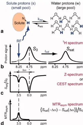
Fig. 1.2 Chemical Exchange Saturation Transfer (CEST). | Principles and measurement approach for pure exchange effects. Adapted from Ref.15

In a typical CEST imaging experiment, there are at-least two unique proton frequency pools.

The water proton usually forms the ‘bulk’ spin pool, whereas protons associated with other

organic groups such as hydroxy, amide, or imine, constitute the second, chemically shifted (𝛿) pool. A typical CEST sequence consists of first ‘destroying’ the MR signal from the second pool

(27)

from the bulk water pool, as a result of exchange into the secondary pool. As long as the exchange rate of protons between the two chemical pools is equivalent or comparable to the

chemical shift between the two resonances, there will be an appreciable loss of ‘bulk’

magnetization signal. As such, CEST MRI is particularly useful for noninvasive imaging of metabolism, tissue composition, and pH.

1.5 Contrast agents in MRI

Despite its unprecedented power and utility for non-invasive anatomical imaging, MRI is fundamentally limited in its sensitivity by a) density and polarization efficacy of nuclear spins, b) diffusion of spins, and c) molecular motion and resulting fast fluctuations in the magnetic field. Contrast agents in MRI, as with other imaging modalities, are therefore used to improve detection of specific molecular processes relative to background.

1.5.1 T1 contrast agents: mechanism of action

One of the principal advantages of T1– weighted MRI over T2– weighted, Diffusion-weighted,

and CEST MRI is that voxels which contain T1 contrast agents appear brighter on T1– weighted images. This ‘positive’ contrast fundamentally results from an acceleration in the T1 of nuclear

spins due to the transient coordination with paramagnetic compounds within the voxel.16_Since

the electron’s gyromagnetic ratio (𝛾𝑒 = 28.02 GHz T⁄ ) is approximately three orders of

magnitude stronger than that of the proton (𝛾_𝐼 = 42.57 MHz T⁄ ), its corresponding thermal polarization is equivalently higher under the same conditions (20℃, 7T).

𝑁aligned

𝑁_{anti−aligned}~𝑒0.0025 → 25000 ppm electron polarization (1.19)

(28)

𝑅_{1 (C.A.)}= 1 𝑇₁~ [

𝛾_𝐼2_𝛾

𝑒2𝑆 ∙ (𝑆 + 1)

𝑟6 ] [

3𝜏_𝐶 1 + 4𝜏_𝐶2_𝜔

𝐿2

] (1.20)

The correlation time for fluctuations in the local fields, as experienced by the nuclear spin, is a function of the rotational correlation time of the paramagnetic molecule, the exchange rate at which spins coordinate and dissociate with the paramagnetic molecule, and the longitudinal relaxation time for the electron spin(s) on the paramagnetic compound (Eq. 1.21a).

1 𝜏𝐶 = 1 𝜏𝑅+ 1 𝜏𝑀+ 1

𝑇1𝑒 (1.21a)

The optimal nuclear spin relaxation in the presence of a paramagnetic T1 contrast agent occurs

when the correlation frequency (_𝜏𝐶1 ) is equivalent or comparable to the Larmor frequency. Typical small-molecule paramagnetic T1 contrast agents have correlation times which are

dominated by molecular tumbling (Eq. 1.21b).

1

𝜏_𝑅~ 2 − 20 GHz, 1

𝜏_𝑀 ~ 100 MHz, and 1

𝑇_1𝑒 ~ 35 MHz at 1.5 T (1.21b)

We can infer from Eq. 1.21a and Eq. 1.21b that the rotational correlation time and exchange rate have the largest influence on the relaxivity of a T1 contrast agent. Previous strategies for

engineering high relaxivity T1 contrast agents have focused on 1) reducing molecular tumbling,

2) engineering ligands around the paramagnetic ion that affect both the proton exchange rate, as well as 3) total electron spin. While all T1 contrast agents also produce T2 effects, these are

modest when compared with T1 contrast. Lastly, while T1 contrast agents continue to be actively

studied in the field, they are not the primary focus of this thesis.17 1.5.2 T2 contrast agents: mechanism of action

The principal advantage of T2 – weighted imaging is that its corresponding MRI pulse sequences

are among the fastest imaging schemes, when compared with other MRI pulse sequences, such as T1 or CEST; consequently T2 imaging has been extensively used for functional in vivo studies.

(29)

developed and can be detected in vivo at pg Fe cell⁄ , approaching sensitivities achieved with PET.18_{Given their sensitivity, as well as speed of detection, the rest of this thesis is focused on} engineering and applying T2 contrast agents to imaging and controlling cellular function

non-invasively.

Unlike T1 contrast agents which primarily relax water protons through direct coordination with

paramagnetic centers (inner-sphere relaxation), T2 contrast agents act by changing the magnetic

susceptibility of the voxel itself; consequently, the effects on MRI contrast of T2 contrast agents

can be felt far beyond the voxel that contains them. As such, any water molecules that diffuse through and around such voxels experience fundamentally different magnetic fields.19–21_The strongest T2 contrast agents are SPIONs, which introduce significant spatial inhomogeneity in

the local magnetic field due to their strong magnetic properties, with saturation magnetization up to (𝑀𝑠𝑎𝑡 ~ 120 emu g⁄ ).

The influence of SPIONs on T2 relaxation depends on both their number density within a voxel

(𝑁 𝑉⁄ ), and the characteristic diffusion timescales of the spins themselves (𝜏𝐷).22 To gain deeper

insight into how these factors affect T2 contrast, we start by modeling the phase accrued by a

nuclear spin as it diffuses past a SPION of radius R with magnetization M. The equatorial z -component of the magnetic field of a SPION of radius R is given by Eq. 1.22.

𝐁_SPION= 𝜇0𝐌

3 (

𝑅 𝑟)

3

(3 cos2_{𝜃 − 1)} _(1.22)

We can define the volume fraction of a voxel occupied by SPIONs as f, wherein

𝑓 =𝑁𝜐

𝑉 (1.23)

(30)

𝑙_𝑠𝑒𝑝 = (𝜐 𝑓)

1 3⁄ = (

4 3 𝜋

𝑓 ) 1 3⁄

𝑅 (1.24)

Over some time 𝜏, nuclear spins diffuse a characteristic distance (𝑙_{𝑑𝑖𝑓𝑓}) as determined by the 3D diffusion equation, where D is the bulk diffusion coefficient of water at room temperature.

𝑙_{𝑑𝑖𝑓𝑓} = √6𝐷𝜏 (1.25)

If the SPIONs are large enough that the characteristic diffusion distance is small when compared with the average inter-particle spacing (𝑙_𝑙𝑑𝑖𝑓𝑓

𝑠𝑒𝑝 ≪ 1) at a fixed volume fraction, then the majority

of spins only experience a single magnetic environment. In this scenario, the inhomogeneous relaxation rate (𝑅₂∗₎_{is unaffected by spin diffusion and near its theoretical maximum. This} ‘single-environment’ regime is classically referred to as the static dephasing regime since field

fluctuations are approximately constant across an MR echo. That said, the loss of phase coherence can be partially reversed by applying a gradient with opposite polarity (spin-echo pulse sequence), which explains why the homogeneous relaxation rate is smaller than the inhomogeneous relaxation rate (𝑅2 < 𝑅2∗) in the static dephasing regime.

On the other hand, if the characteristic diffusion distance is large when compared with the inter-particle separation distance (𝑙_𝑙𝑑𝑖𝑓𝑓

𝑠𝑒𝑝 ≫ 1) at a fixed volume fraction, then spins will sample

multiple magnetic fields, including those with opposite polarity, within an MR echo. This scenario is referred to as the motional averaging regime, in which the inhomogeneous relaxation rate (𝑅₂∗₎_{can be analytically solved (Eq. 1.26a) from the SBM equations. Additionally, nuclear}

spin relaxation by SPIONs is referred to as Outer-sphere (OS) relaxation since it requires no direct coordination between the nuclei and the nanoparticle, which also explains how T2 contrast

agents exert their influence across large distances.

𝑅₂∗ ₌4

(31)

∆𝜔₀ = 𝛾𝐁_SPION (1.26b)

𝜏𝐷 = 𝑅2⁄𝐷 (1.26c)

Here, ∆𝜔₀ refers to the shift in proton Larmor frequency at the equator of the SPION and 𝜏_𝐷

is the characteristic time needed for spins to diffuse into a new magnetic environment. Since the MRI signal is effectively lost when its phase discrepancy exceeds 90°, (|∆𝜙| ≥ 𝜋 2⁄ ), we can deduce the effective timescale of spin coherence (𝜏_𝑅) as follows.

𝜋

2 = 𝛾〈|𝐁𝐒𝐏𝐈𝐎𝐍|〉𝜏𝑅 (1.27)

We can estimate the average magnitude of the magnetic field (z-component) produced by a SPION by integrating out all its angular components at a fixed radius r and obtain:

〈|𝐁𝐒𝐏𝐈𝐎𝐍|〉 ≈ 𝜇₀𝐌

6 (

𝑅 𝑟)

3

(1.28)

We can then estimate the characteristic timescale of spin coherence to be23

𝜏_𝑅 ≈ 3𝜋 𝜇₀𝛾𝐌(

𝑟 𝑅)

3

(1.29)

Equating the time needed for a spin to diffusively sample the field profile of a SPION (𝜏_𝐷) with the time taken for spin-phase to become completely incoherent (𝜏_𝑅), enables us to estimate the distance over which a SPION influences the phase of all nuclear spins (Eq. 1.30). Spins outside

this ‘boundary’ remain coherent, whereas those that diffuse into this region will experience field

inhomogeneities and faster T2* relaxation.

𝑙_{𝑏𝑜𝑢𝑛𝑑𝑎𝑟𝑦} ≈𝜇0𝛾𝐌

3𝜋𝐷 𝑅3 (1.30)

(32)

of influence (𝑙_{𝑏𝑜𝑢𝑛𝑑𝑎𝑟𝑦}) before being fully dephased, whereas particles larger than this size will fully relax spins within a single encounter.

𝑅_{𝑐𝑟𝑖𝑡} ≈ √3𝜋𝐷

𝜇₀𝛾𝐌 (1.31)

Using typical values for the volume magnetization and water diffusion coefficient, Eq. 1.38 suggests that the critical particle size is approximately around 20 nm. For SPIONs much larger than this critical size, such as 200 nm SPIONs, their zone of influence scales as the cube of particle radius (𝑙_{𝑏𝑜𝑢𝑛𝑑𝑎𝑟𝑦} ~ 10 μm), which suggests that protons have to diffuse quite far before encountering a new magnetic environment. Unless spins are close to the large SPION surface, they will experience relatively shallow field inhomogeneities whose effects on signal phase can be reversed using a refocusing pulse. Consequently, these simple scaling arguments suggest that the optimal T2 contrast is achieved using SPIONS that are approximately 20 – 50

nm in size.24_{It is therefore unsurprising that SPIONs within this size regime are the most} extensively used contrast agents for in vivo imaging studies.

1.5.3 Genetically encoded T2 contrast agents

(33)

parallel efforts to exploit other endogenous metalloproteins that can also produce T2 contrast

in vivo, albeit weakly.35 – 41

Accordingly, one popular chassis for engineering has been the metalloprotein ferritin, which is an 8nm particle that can hold up to 4500 Fe atoms under optimal iron-loading. Ferritin is thought to have evolved as atmospheric concentrations of oxygen rose, and acts as an iron storage and ferrous-iron detoxification vehicle for cells (prokaryotes, archaea, and eukaryotes).42 - 43_Unlike microbial magnetosomes which biosynthesize superparamagnetic iron oxides such as magnetite, iron in ferritins is stored as a mixture of weakly paramagnetic and antiferromagnetic iron oxides under ambient conditions.44 – 47

Furthermore, unlike SPIONs whose relaxivity saturates at fields higher than 1 Tesla, ferritins exhibit a linear increase in relaxivity with increasing field strength. This interesting deviation from conventional outer-sphere relaxation theory (Sec. 1.5.2) is thought to arise from proton-exchange driven dephasing.48 – 50_{Freely diffusing water protons weakly adsorb onto the} paramagnetic ferrihydrite surface within the ferritin core, and lose phase through dipolar interactions with paramagnetic ferric ions. Since the ferrihydrite mineral is intrinsically disordered, protons experience a broad (Lorentzian) distribution of magnetic fields.51 – 53_Lastly, the relaxivity of ferritins is fundamentally limited by 1) water access to the ferrihydrite mineral and 2) the net paramagnetic moment of the mineral itself, which scales as √𝑁Fe.54

The ferroxidase center of all known ferritins sits at the interface of two alpha-helical subunits, and uses molecular oxygen as the terminal electron acceptor to oxidize ferrous iron into ferric

iron, which is then shuttled into the nanoparticle’s interior using an electrostatic potential

(34)

nascent iron-oxide mineral within the nanoparticle, thus producing mixed valence and intrinsically disordered phospho-ferrihydrite. The bulk of this mineral, however, is antiferromagnetically spin-coupled, and any paramagnetism that results can be accounted for by the incomplete cancellation of canted, surface electrons. As such, only 5% (at most) of the total iron contained within ferritins contributes to its overall paramagnetic moment.54

Ferritins are fundamentally unable to mineralize superparamagnetic iron-oxides in living cells due to 1) passive control of interior pH, 2) unsuitable control of iron redox stoichiometry, and 3) unstructured mineralization of iron-oxides. Interestingly, initial experiments with apo-ferritin demonstrated that if the pH, concentration of oxygen, and concentration of ferrous iron could be controlled, then ferritins were indeed capable of nucleating magnetite within their cores, thereby producing a 8 nm SPION with ~ 40 fold improvement in T2 relaxivity.59 – 61 Accordingly,

over the last three decades, considerable efforts have been directed towards engineering and evolving ferritins to generate variants that are capable of nucleating magnetite in living cells. While such studies have produced ferritin variants with slightly different oxidation rates and mineralization capacity, they have not been successful in producing a truly superparamagnetic nanoparticle under typical cellular conditions.

This is primarily because the rate-limiting criteria for magnetite synthesis are redox-potential and pH.62_{In this light, it is unsurprising that magnetotactic bacteria first create lipid-enclosed} nano-compartments in which the pH and redox properties of iron can be tightly controlled, prior to iron import and mineral nucleation.63-64_{The conditions within these magnetosome} compartments are thermodynamically permissive for the spontaneous nucleation and growth of magnetite, once a critical amount of ferrous and ferric iron is introduced.65–67_{On the other hand,} the typical redox and pH conditions within the mammalian or even most aerobic prokaryotic cytoplasm favor the formation of mixed valence ferrihydrites and non-magnetic iron-oxides.68 1.5.4 Engineering paramagnetic cells as T2 contrast agents

Given the fundamental thermodynamic and chemical constraints that prevent the biomineralization of magnetite and other ferromagnetic iron oxides within the mammalian and

(35)

Previous efforts towards engineering strongly paramagnetic ferritins69 – 74_{demonstrated that if} a cell had enough paramagnetic metalloproteins, then it could be 1) visualized in vivo using MRI and 2) captured in vitro using strong magnetic field gradients.71,72,75_{This is unsurprising given that} the magnetic susceptibility of most tissues is within ± 10 − 20% of that of water; consequently, the paramagnetism wrought by even a single paramagnetic ion, such as Fe3+_{, is sufficient to} overcome the diamagnetic contribution from hundreds of thousands of water molecules. In the case of ferritins, if one assumes an ideal, fully loaded particle with 4500 Fe3+_{high-spin iron atoms} (𝑆 =5₂) and a diamagnetic protein shell, the magnetic susceptibility of a voxel with a single particle is significantly more paramagnetic (Eq. 1.32).

𝜒_{𝑓𝑒𝑟𝑟𝑖𝑡𝑖𝑛} ~ 520 × 10−6 _(1.32)

While it is unlikely to observe this high degree of loading and spin-state in cells given the high concentration of endogenous iron chelators, the susceptibility of liver tissue in instances of iron-overload disease was calculated to be approximately 𝜒_{ℎ𝑒𝑚𝑎𝑐ℎ𝑟𝑜𝑚𝑎𝑡𝑜𝑠𝑖𝑠}~ 10−5_{, based on iron}

levels of approximately 6.6 mg Fe/g.8_{This reinforces the notion that a reasonable quantity of}

paramagnetic material is sufficient to shift an MRI voxel’s magnetic susceptibility by a few ppm,

thus enabling more sensitive MRI detection, as well as magnetic capture.

(36)

BIBLIOGRAPHY

1. Piraner, D. I. et al. Going Deeper: Biomolecular Tools for Acoustic and Magnetic Imaging and Control of Cellular Function. Biochemistry 56, 5202–5209 (2017).

2. Mukherjee, A., Davis, H. C., Ramesh, P., Lu, G. J. & Shapiro, M. G. Biomolecular MRI reporters: Evolution of new mechanisms. Prog. Nucl. Magn. Reson. Spectrosc. 102, 32–42 (2017).

3. Thorek, D. L. J., Chen, A. K., Czupryna, J. & Tsourkas, A. Superparamagnetic iron oxide nanoparticle probes for molecular imaging. Ann. Biomed. Eng. 34, 23–38 (2006).

4. Kellogg, J. M. B., Rabi, I. I. & Zacharias, J. R. The gyromagnetic properties of the hydrogens. Phys. Rev. 50, 472–481 (1936).

5. Bloch, F. Nuclear Induction. Phys. Rev. Lett. 70, 127–127 (1946).

6. Bloembergen, N., Purcell, E. M. & Pound, R. V. Relaxation Effects in Nuclear Magnetic Resonance Absorption. Phys. Rev. Lett. 73, (1947).

7. Plewes, D. B. & Kucharczyk, W. Physics of MRI: a primer. J. Magn. Reson. Imaging 35, 1038–54 (2012).

8. Schenck, J. F. The role of magnetic susceptibility in MRI. Med. Phys. 23, (1996). 9. Kittel, C. Physical Theory of Ferromagnetic Domains. Rev. Mod. Phys. 21, (1949).

10. Szotek, Z. et al. Electronic structures of normal and inverse spinel ferrites from first principles. Phys. Rev. B - Condens. Matter Mater. Phys. 74, 1–12 (2006).

11. Lee, J.-H. et al. Artificially engineered magnetic nanoparticles for ultra-sensitive molecular imaging. Nat. Med. 13, 95–99 (2007).

12. Lu, X. et al. Ultrashort Echo Time Quantitative Susceptibility Mapping (UTE-QSM) of Highly Concentrated Magnetic Nanoparticles: A Comparison Study about Different Sampling Strategies. Molecules 24, 1143 (2019).

13. Chen, R., Christiansen, M. G. & Anikeeva, P. Maximizing hysteretic losses in magnetic ferrite nanoparticles via model-driven synthesis and materials optimization. ACS Nano 7, 8990–9000 (2013).

14. Keeler, J. & Pell, A. J. Understanding NMR Spectroscopy, Second Edition. (Wiley, 2010). 15. Van Zijl, P. C. M. & Yadav, N. N. Chemical exchange saturation transfer (CEST): What

is in a name and what isn’t? Magn. Reson. Med. 65, 927–948 (2011).

16. Lauffer, R. E. Paramagnetic Metal Complexes as Water Proton Relaxation Agents for NMR Imaging : Theory and Design. Chem. Rev. 87, (1987).

17. Shapiro, M. G. et al. Directed evolution of a magnetic resonance imaging contrast agent for noninvasive imaging of dopamine. Nat. Biotechnol. 28, 264–270 (2010).

18. Heyn, C., Bowen, C. V., Rutt, B. K. & Foster, P. J. Detection threshold of single SPIO-labeled cells with FIESTA. Magn. Reson. Med. 53, 312–320 (2005).

(37)

Magn. Reson. Med. 57, 442–447 (2007).

20. Brooks, R. A. T2-Shortening by Strongly Magnetized Spheres: A Chemical Exchange Model. Magn. Reson. Med. 47, 257–263 (2002).

21. Brown, K. A. et al. Scaling of transverse nuclear magnetic relaxation due to magnetic nanoparticle aggregation. J. Magn. Magn. Mater. 322, 3122–3126 (2010).

22. Vuong, Q. L., Gossuin, Y., Gillis, P. & Delangre, S. New simulation approach using classical formalism to water nuclear magnetic relaxation dispersions in presence of superparamagnetic particles used as MRI contrast agents. J. Chem. Phys. 137, 0–13 (2012). 23. De Haan, H. W. Mechanisms of proton spin dephasing in a system of magnetic particles.

Magn. Reson. Med. 66, 1748–1758 (2011).

24. Vuong, Q. L., Berret, J. F., Fresnais, J., Gossuin, Y. & Sandre, O. A universal scaling law to predict the efficiency of magnetic nanoparticles as MRI T2-contrast agents. Adv. Healthc. Mater. 1, 502–512 (2012).

25. Shapiro, M. G., Atanasijevic, T., Faas, H., Westmeyer, G. G. & Jasanoff, A. Dynamic imaging with MRI contrast agents: quantitative considerations. Magn. Reson. Imaging 24, 449–62 (2006).

26. Shapiro, M. G., Szablowski, J. O., Langer, R. & Jasanoff, A. Protein nanoparticles engineered to sense kinase activity in MRI. J. Am. Chem. Soc. 131, 2484–2486 (2009). 27. Rahn-Lee, L. & Komeili, A. The magnetosome model: insights into the mechanisms of

bacterial biomineralization. Front. Microbiol. 4, 352 (2013).

28. Arakaki, A., Nakazawa, H., Nemoto, M., Mori, T. & Matsunaga, T. Formation of magnetite by bacteria and its application. J. R. Soc. Interface 5, 977–99 (2008).

29. Lefèvre, C. T. et al. Monophyletic origin of magnetotaxis and the first magnetosomes.

Environ. Microbiol. 15, 2267–2274 (2013).

30. Uebe, R. & Schüler, D. Magnetosome biogenesis in magnetotactic bacteria. Nat. Rev. Microbiol. 14, 621–637 (2016).

31. Komeili, A. Molecular Mechanisms of Compartmentalization and Biomineralization in Magnetotactic Bacteria. FEMS Microbiol. Rev. 36, 232–255 (2012).

32. Murat, D., Quinlan, A., Vali, H. & Komeili, A. Comprehensive genetic dissection of the magnetosome gene island reveals the step-wise assembly of a prokaryotic organelle. Proc. Natl. Acad. Sci. U. S. A. 107, 5593–8 (2010).

33. Kolinko, I. et al. Biosynthesis of magnetic nanostructures in a foreign organism by transfer of bacterial magnetosome gene clusters. Nat. Nanotechnol. 9, 193–197 (2014). 34. Lohsse, A. et al. Functional analysis of the magnetosome island in Magnetospirillum

gryphiswaldense: the mamAB operon is sufficient for magnetite biomineralization. PLoS One 6, e25561 (2011).

35. Sigmund, F. et al. Bacterial encapsulins as orthogonal compartments for mammalian cell engineering. Nat. Commun. 9, 1990 (2018).

36. Patrick, P. S. et al. Development of Timd2 as a reporter gene for MRI. Magn. Reson. Med.

(38)

37. Iordanova, B., Hitchens, T. K., Robison, C. S. & Ahrens, E. T. Engineered Mitochondrial Ferritin as a Magnetic Resonance Imaging Reporter in Mouse Olfactory Epithelium. PLoS One 8, (2013).

38. Pereira, S. M. et al. Evaluating the effectiveness of transferrin receptor-1 ( TfR1 ) as a magnetic resonance reporter gene. Contrast Media Mol. Imaging n/a-n/a (2016). doi:10.1002/cmmi.1686

39. Bartelle, B. B., Szulc, K. U., Suero-Abreu, G. a, Rodriguez, J. J. & Turnbull, D. H. Divalent metal transporter, DMT1: A novel MRI reporter protein. Magn. Reson. Med.000, 1–9 (2012).

40. Genove, G., DeMarco, U., Xu, H., Goins, W. F. & Ahrens, E. T. A new transgene reporter for in vivo magnetic resonance imaging. Nat. Med. 11, 450–4 (2005).

41. Iordanova, B. & Ahrens, E. T. In vivo magnetic resonance imaging of ferritin-based reporter visualizes native neuroblast migration. Neuroimage 59, 1004–1012 (2012). 42. Chasteen, N. D. & Harrison, P. M. Mineralization in ferritin: an efficient means of iron

storage. J. Struct. Biol. 126, 182–194 (1999).

43. Bou-Abdallah, F. The iron redox and hydrolysis chemistry of the ferritins. Biochim. Biophys. Acta - Gen. Subj. 1800, 719–731 (2010).

44. Pan, Y. H. et al. 3D morphology of the human hepatic ferritin mineral core: New evidence for a subunit structure revealed by single particle analysis of HAADF-STEM images. J. Struct. Biol. 166, 22–31 (2009).

45. García-Prieto, A. et al. On the mineral core of ferritin-like proteins: structural and magnetic characterization. Nanoscale 8, 1088–1099 (2016).

46. Lid, S., Carmona, D., Maas, M., Treccani, L. & Colombi Ciacchi, L. Anchoring of Iron Oxyhydroxide Clusters at H and L Ferritin Subunits. ACS Biomater. Sci. Eng. 4, 483–490 (2018).

47. Brem, F., Stamm, G. & Hirt, A. M. Modeling the magnetic behavior of horse spleen ferritin with a two-phase core structure. J. Appl. Phys. 99, (2006).

48. Gossuin, Y., Roch, A., Muller, R. N., Gillis, P. & Lo Bue, F. Anomalous nuclear magnetic relaxation of aqueous solutions of ferritin: An unprecedented first-order mechanism.

Magn. Reson. Med. 48, 959–964 (2002).

49. Brooks, R. A. et al. Relaxometry and magnetometry of ferritin. Magn. Reson. Med. 40, 227–

235 (1998).

50. Brooks, R. A., Moiny, F. & Gillis, P. On T2-shortening by weakly magnetized particles: The chemical exchange model. Magn. Reson. Med. 45, 1014–1020 (2001).

51. Michel, F. M. et al. The Structure of Ferrihydrite, a Nanocrystalline Material. Science (80-. ). 316, 1726–1729 (2007).

52. Murad, E. & Schwertmann, U. The Mössbauer spectrum of ferrihydrite and its relations to those of other iron oxides. Am. Mineral. 65, 1044–1049 (1980).

(39)

(2010).

54. Harris, J. G. E., Grimaldi, J. E., Awschalom, D. D., Chiolero, a. & Loss, D. Excess Spin and the Dynamics of Antiferromagnetic Ferritin. 60, 4 (1999).

55. Douglas, T. & Ripoll, D. R. Calculated electrostatic gradients in recombinant human H-chain ferritin. Protein Sci. 7, 1083–1091 (1998).

56. Bradley, J. M. et al. Three aromatic residues are required for electron transfer during iron mineralization in bacterioferritin. Angew. Chemie - Int. Ed. 54, 14763–14767 (2015). 57. Behera, R. K. et al. Fe2+ substrate transport through ferritin protein cage ion channels

influences enzyme activity and biomineralization. JBIC J. Biol. Inorg. Chem. 20, 957–969 (2015).

58. Bou-Abdallah, F. et al. Functionality of the three-site ferroxidase center of Escherichia coli bacterial ferritin (EcFtnA). Biochemistry 53, 483–95 (2014).

59. Clavijo Jordan, V., Caplan, M. R. & Bennett, K. M. Simplified synthesis and relaxometry of magnetoferritin for magnetic resonance imaging. Magn. Reson. Med. 64, 1260–1266 (2010).

60. Meldrum, F. C., Heywood, B. R. & Mann, S. Magnetoferritin: in vitro synthesis of a novel magnetic protein. Science 257, 522–523 (1992).

61. Martínez-Pérez, M. J. et al. Size-dependent properties of magnetoferritin. Nanotechnology

21, 465707 (2010).

62. Baumgartner, J. et al. Nucleation and growth of magnetite from solution. Nat. Mater. 12, 310–314 (2013).

63. Baumgartner, J. et al. Magnetotactic bacteria form magnetite from a phosphate-rich ferric hydroxide via nanometric ferric (oxyhydr)oxide intermediates. Proc. Natl. Acad. Sci. U. S. A. 1, (2013).

64. Moisescu, C., Ardelean, I. I. & Benning, L. G. The effect and role of environmental conditions on magnetosome synthesis. Front. Microbiol. 5, 1–12 (2014).

65. Murat, D. et al. The magnetosome membrane protein, MmsF, is a major regulator of magnetite biomineralization in Magnetospirillum magneticum AMB-1. Mol. Microbiol.85, 684–99 (2012).

66. Arakaki, A., Yamagishi, A., Fukuyo, A., Tanaka, M. & Matsunaga, T. Coordinated functions of Mms proteins define the surface structure of cubo-octahedral magnetite crystals in magnetotactic bacteria. Mol. Microbiol. 93, 1–30 (2014).

67. Fdez-Gubieda, M. L. et al. Magnetite Biomineralization in Magnetospirillum gryphiswaldense: Time-Resolved Magnetic and Structural Studies ). ACS Nano 7, 3297–

3305 (2013).

68. Kosman, D. J. Iron metabolism in aerobes: Managing ferric iron hydrolysis and ferrous iron autoxidation. Coord. Chem. Rev. 257, 210–217 (2013).

(40)

Directed Evolution. Sci. Rep. 6, 1–10 (2016).

71. Kim, T., Moore, D. & Fussenegger, M. Genetically programmed superparamagnetic behavior of mammalian cells. J. Biotechnol. 162, 237–45 (2012).

72. Nishida, K. & Silver, P. a. Induction of biogenic magnetization and redox control by a component of the target of rapamycin complex 1 signaling pathway. PLoS Biol. 10, e1001269 (2012).

73. Radoul, M. et al. Genetic manipulation of iron biomineralization enhances MR relaxivity in a ferritin-M6A chimeric complex. Sci. Rep. 6, 1–9 (2016).

74. Iordanova, B., Robison, C. S. & Ahrens, E. T. Design and characterization of a chimeric ferritin with enhanced iron loading and transverse NMR relaxation rate. J. Biol. Inorg. Chem. 15, 957–965 (2010).

75. Xie, H. et al. A quantitative study of susceptibility and additional frequency shift of three common materials in MRI. Magn. Reson. Med. 00, n/a-n/a (2015).

76. Vuong, Q. L. et al. Paramagnetic nanoparticles as potential MRI contrast agents: Characterization, NMR relaxation, simulations and theory. Magn. Reson. Mater. Physics, Biol. Med. 25, 467–478 (2012).