Topics in Theoretical Particle Physics and Cosmology
Thesis by
Michael P. Salem
In Partial Fulfillment of the Requirements for the Degree of
Doctor of Philosophy
California Institute of Technology Pasadena, California
2007
c
2007
Acknowledgements
Much of this research would not have occurred without the hard work and insight of my collaborators. For this I thank Christian Bauer, Matthew Dorsten, Michael Graesser, Lawrence Hall, and Taizan Watari. I have been fortunate to have collaborators who were all willing to patiently explain ideas within and beyond the scope of our research. For this I am especially grateful to Christian, Michael, and Taizan, who have greatly increased my understanding of theoretical physics.
I am pleased to acknowledge my graduate adviser Mark Wise, who has provided invaluable guidance and support throughout my graduate studies. I have benefited much from his suggestions and his pedagogy, while his humor and congeniality helped make graduate school a very enjoyable experience. For his guidance and support I am also grateful to my undergraduate adviser Tanmay Vachaspati. His clever ideas initiated a successful collaboration on my undergraduate thesis, which set the stage for my subsequent progress. I am grateful that both of my advisers have always received me warmly and respectfully.
I have learned much from the other members of Mark’s research group. For this I thank Lotty Ackerman, Moira Gresham, Alejandro Jenkins, Jennifer Kile, Sonny Mantry, Donal O’Connell, Sean Tulin, and Peng Wang. Lotty, Moira, and Donal have been especially patient and helpful in answering my questions. I have also benefited from interactions with Michael Ramsey-Musolf, Marc Kamionkowski, and members of Marc’s research group, in particular Jonathan Pritchard and Kris Sigurdson. All of these people helped to create a pleasant and productive working environment. For this I am also grateful to my previous and present officemates, in particular Paul Cook and Jie Wang and especially Moira Gresham.
Through most of my graduate studies I have been financially supported primarily by a Caltech teaching assistantship. I am thankful to David Goodstein and especially David Politzer and my Ph1 students for making this responsibility an enjoyable learning experience. I have also received financial support via the Caltech department of physics, the John A. McCone Chair, and the U.S. Department of Energy under contract number DE-FG03-92ER40701. I am grateful to Carol Silberstein and Charlene Cartier for their friendliness and their extensive administrative support.
together has made my life and my work all the more rewarding. For these, and everything else Sara gives, I am endlessly grateful. I am also thankful for my siblings, Jeff, Joe, Karen, and Sherry, their spouses Jason and Mark, and my parents Frank and Marie. Their constant praise has encouraged me throughout my studies. More importantly, they contributed most to make me who I am.
Abstract
We first delve into particle phenomenology with a study of soft-collinear effective theory (SCET), an effective theory for Quantum Chromodynamics for when all particles are approximately on their light-cones. In particular, we study the matching of SCETI involving ultrasoft and collinear particles
onto SCETII involving soft and collinear particles. We show that the modes in SCETII are sufficient
to reproduce all of the infrared divergences of SCETI, a result that was previously in contention.
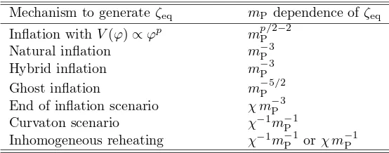
Next we move into early universe cosmology and study alternative mechanisms for generating primordial density perturbations. We study the inhomogeneous reheating mechanism and extend it to describe the scenario where the freeze-out process for a heavy particle is modulated by sub-dominant fields that received fluctuations during inflation. This scenario results in perturbations that are comparable to those generated by the original inhomogeneous reheating scenarios. In addition, we study yet another alternative to single field inflation whereby the curvature perturbation is generated by interactions at the end of inflation, as opposed to when inflaton modes exit the horizon. We clarify the circumstances under which this process can dominate over the standard one and we show that it may result in a spectrum with an observable level of non-Gaussianities.
Contents
Acknowledgements iii
Abstract v
1 Introduction 1
1.1 Soft-Collinear Effective Theory . . . 1
1.2 Alternative Mechanisms to Generate Primordial Density Perturbations . . . 5
1.3 Low-Energy Consequences of a Landscape . . . 12
2 Infrared Regulators and SCETII 17 2.1 Introduction . . . 17
2.2 Matching from SCETI onto SCETII . . . 19
2.3 Infrared Regulators in SCET . . . 23
2.3.1 Problems with Known IR Regulators . . . 23
2.3.2 A New Regulator for SCET . . . 25
2.4 Conclusions . . . 28
3 Fluctuating Annihilation Cross Sections and the Generation of Density Pertur-bations 30 3.1 Introduction . . . 30
3.2 Analytical Determination of the Perturbations . . . 32
3.3 Explicit Models for CouplingS to Radiation . . . 34
3.4 Models for Producing the Fluctuations . . . 36
3.5 Evolution of Density Perturbations . . . 39
3.6 Numerical Results . . . 41
3.7 Conclusions . . . 42
4 On the Generation of Density Perturbations at the End of Inflation 44 4.1 Introduction . . . 44
4.3 The Specific Model . . . 47
4.4 A More Detailed Analysis . . . 48
4.5 Generalizing the Model . . . 52
4.5.1 Varying the Potential forφ . . . 52
4.5.2 Relaxing the Constraint onλσ . . . 53
4.6 Discussion and Conclusions . . . 55
5 The Scale of Gravity and the Cosmological Constant within a Landscape 57 5.1 Introduction . . . 57
5.2 Anthropic Constraints on the Scale of Gravity . . . 61
5.2.1 Inflation . . . 63
5.2.1.1 Satisfying Slow-Roll forN e-folds of Inflation . . . 63
5.2.1.2 The Curvature Perturbationζ . . . 63
5.2.1.3 Reheating . . . 65
5.2.2 Baryogenesis . . . 65
5.2.3 Big Bang Nucleosynthesis . . . 67
5.2.4 Matter Domination . . . 68
5.2.5 Structure Formation . . . 70
5.2.5.1 Halo Virialization . . . 72
5.2.5.2 Galaxy Formation . . . 73
5.2.5.3 Star Formation . . . 75
5.2.6 Stellar Dynamics . . . 77
5.2.6.1 Stellar Lifetimes and Spectra . . . 78
5.2.6.2 Heavy Element Production . . . 81
5.2.7 Stability of Stellar Systems . . . 82
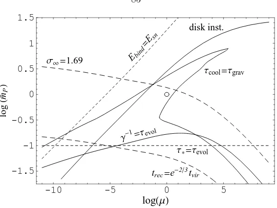
5.2.8 Summary . . . 85
5.3 The Probability Distribution for the Scale of Gravity . . . 88
5.4 Anthropic Constraints on Λ and the Scale of Gravity . . . 93
5.5 Nonstandard Paths toward Structure Formation . . . 99
5.6 Analysis of a Structure Formation Constraint . . . 101
5.7 Conclusions . . . 104
6 Quark Masses and Mixings from the Landscape 106 6.1 Introduction . . . 106
6.2 Prelude: Hierarchy without Flavor Symmetry . . . 109
6.2.1 The Distribution of Mass Eigenvalues . . . 110
6.2.3 Problems . . . 115
6.3 A Toy Landscape: Quarks in One Extra Dimension . . . 115
6.3.1 Emergence of Scale-Invariant Distributions . . . 116
6.3.2 Quark-Sector Phenomenology of the Gaussian Landscape . . . 120
6.3.3 Environmental Selection Effects . . . 124
6.3.4 Summary . . . 125
6.4 Testing Landscape Model Predictions . . . 127
6.4.1 The Chi-Square Statistic . . . 128
6.4.2 The P-Value Statistic . . . 129
6.5 Geometry Dependence . . . 131
6.5.1 A Gaussian Landscape onT2 . . . 131
6.5.2 Changing the Number of Dimensions . . . 133
6.5.3 Information Not Captured by the Number of Dimensions . . . 137
6.6 Approximate Probability Distribution Functions . . . 140
6.6.1 Gaussian Landscape with One Extra Dimension . . . 140
6.6.2 Gaussian Landscapes onD= 2 andD= 3 usingfD(y) in Eq. (6.61) . . . 141
6.7 Discussion and Conclusions . . . 143
List of Figures
2.1 Diagrams in SCETI that contribute to the matching . . . 20
2.2 Diagrams in SCETII that contribute to the matching . . . 20
2.3 Contribution of the proposed additional SCETII mode . . . 21
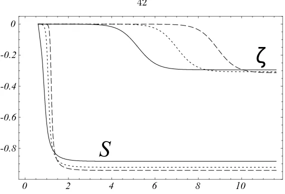
3.1 Evolution ofS andζ in units ofδhσvi as a function of log(mS/T) . . . 42
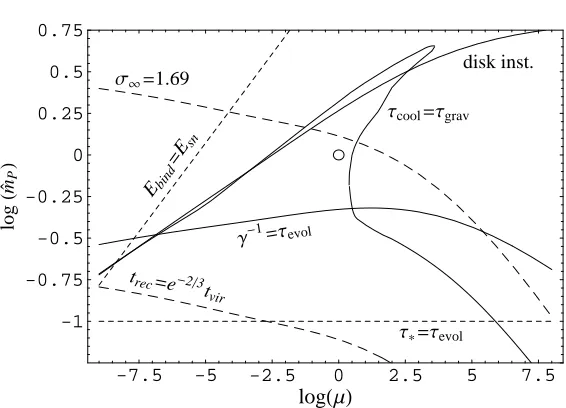
5.1 Anthropic constraints on ˆmP as a function ofµforα= 1 andβ = 0 . . . 85
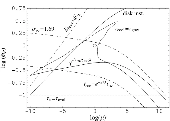
5.2 Anthropic constraints on ˆmP as a function ofµforα= 1 andβ = 3/2 . . . 86
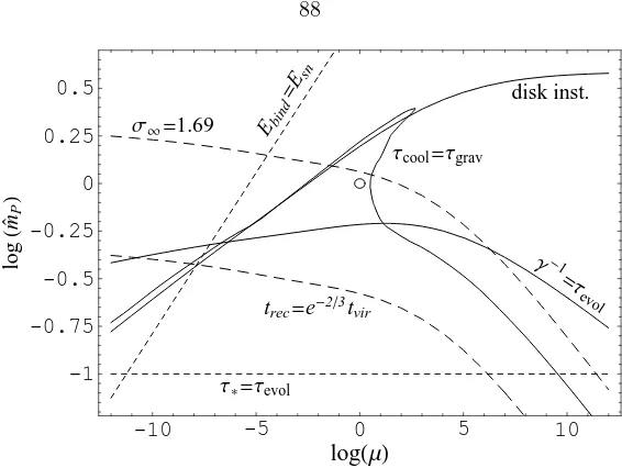
5.3 Anthropic constraints on ˆmP as a function ofµforα= 3 andβ = 0 . . . 87
5.4 Anthropic constraints on ˆmP as a function ofµforα= 3 andβ = 3/2 . . . 88
5.5 The distributionP(ˆρΛ) displayed against log(ˆρΛ) . . . 97
5.6 The distributionP( ˆmP) when the landscape distribution formP depends on the infla-tionary expansion factor . . . 102
6.1 Distribution of the quark Yukawa eigenvalues without correlations . . . 111
6.2 Approximate distribution of quark Yukawa eigenvalues and mixing angles without cor-relations . . . 112
6.3 Distribution of the three CKM mixing angles without correlations . . . 113
6.4 Distribution of randomly generated Yukawa matrix elements onS1 . . . 119
6.5 Distribution of quark Yukawa eigenvalues and CKM mixing angles onS1 . . . 120
6.6 Distribution of the AFS suppression factors onS1 . . . 121
6.7 Distribution of quark Yukawa eigenvalues onS1, witht-cut . . . 125
6.8 Distribution of CKM mixing angles onS1, witht-cut . . . 126
6.9 Typical values of several flavor parameters onS1 . . . 128
6.10 Distribution of randomly generated Yukawa matrix elements onT2. . . 132
6.11 Distribution of quark Yukawa eigenvalues onT2 . . . 133
6.12 Distribution of CKM mixing angles onT2 . . . 134
6.13 Comparing distribution functions overD= 1,2, and 3 dimensions . . . 137
6.15 Distribution of randomly generated Yukawa matrix elements onS2 . . . 139
Chapter 1
Introduction
This thesis includes all of the published work resulting from my graduate studies at Caltech (and some work to be published in the near future). Since my interests have shifted during these studies, there is no unifying theme that relates all of the chapters in this thesis. Therefore each subject of investigation is presented as a separate chapter with no attempt to unify this work as a whole. To serve as an introduction to this work, a brief background discussion to each of the major topics covered in this thesis is included in the sections below.
1.1
Soft-Collinear Effective Theory
My graduate studies began with an investigation into soft-collinear effective theory (SCET), an effective theory for Quantum Chromodynamics (QCD). A slightly edited version of the publication resulting from this work appears as Chapter 2 of this thesis. In what follows I provide background to this work and describe its context. This involves supplying very brief introductions to SCET and to heavy quark effective theory (HQET). More in-depth descriptions of SCET and HQET can be found in the references cited below. At the end of this section I describe my personal contributions to the work presented in Chapter 2.
We start with a brief description of SCET. The reason for seeking an effective theory for QCD in the first place is that at the energy scales associated with hadrons the QCD coupling “constant” αs is of order unity. This makes it very difficult to study QCD perturbatively at these energies.
SCET [1, 2, 3, 4] identifies a different perturbative quantity that can sometimes be used to study QCD interactions. Specifically, in many QCD interactions the invariant four-momentum dot productp2
for the constituent particles involved in an interaction is much less than then square of the interaction energyQ2. This hierarchy can be parameterized using the small quantity λ, with p2∼Q2λ2. We
can then study QCD perturbatively with respect to an expansion in powers ofλ.
It is convenient to work in light-cone coordinates which refer to the light-cone four-vectorsnand ¯
n, with n2 = ¯n2 = 0 and n
would follow the four-vectorsn= (1,0,0,1) and ¯n= (1,0,0,−1) where the first component is the time component). In these coordinates the components of a general four-momentum are written
pµ= (n·p, n¯·p, p⊥)≡(p+, p−, p⊥), (1.1)
where p⊥ ≡ p− 1
2(¯n·p)n− 1
2(n·p)¯n. In this notation p
2 = p+p−+p2
⊥ from which we can see that for off-shellness p2
∼Q2λ2 we may have pµ
∼ Q(λ2,1, λ) or pµ
∼ Q(λ, λ, λ). The former are referred to as collinear momenta and denoted with a subscript c while the latter are referred to as soft momenta are are denoted with a subscripts. Since adding a single soft momentum to a single collinear momentum takes the latter further off-shell (by increasing thep+ component of the
momentum), soft-collinear interactions must involve at least two soft and two collinear particles. On the other hand, a single collinear particle may directly couple to what is referred to as an ultrasoft (usoft) particle, which is defined by the momenta scalingpµ
∼Q(λ2, λ2, λ2) and which is denoted
with the subscriptus.
The SCET Lagrangian is obtained by integrating out collinear momenta from the QCD La-grangian. The use of light-cone coordinates is pivotal for making the power counting inλmanifest. We first writepµ
c = ˜pµ+kµ where ˜pµ= 12p−n
µ+pµ
⊥ includes the large components of the collinear momentum andkµ includes everything else. Fermions can then be expanded according to
ψ(x) =X
˜
p
e−ip˜·xψn,p˜(x) =
X
˜
p
e−ip˜·x[ξn,p˜(x) +ξn,¯p˜(x)], (1.2)
whereξn,¯p˜≡ 14n/n/ψ¯ n,p˜andξn,p˜≡ 14n/¯n/ψn,p˜are projections of the original fermion onto its collinear
and anti-collinear components. The next step in elucidating the power-counting is to separate the gluon fields into collinear, soft, and usoft componentsAµ =Aµ
c +Aµs+Aµus, where the components
are separated so as to satisfy the power-counting
Aµ
c ∼Q(λ2,1, λ), Aµs ∼Q(λ, λ, λ), Aµus∼Q(λ2, λ2, λ2). (1.3)
Furthermore, the large collinear momenta of Aµ
c are factorized analogously to those of ψ as in
Eq. (1.2). When the QCD Lagrangian is written in terms ofξn,¯p˜, ξn,p˜, Ac,As, andAus, one finds
that at leading order the fieldξn,¯p˜does not interact with soft or usoft degrees of freedom. Therefore
at tree level the field ξn,¯p˜ can be replaced by substituting the solution to its equation of motion.
Putting all of this together gives the leading-order SCET Lagrangian,
LSCET=
X
˜
p,q˜
e−i( ˜p−q˜)·xξ¯n,q˜
in·D+ (˜p/⊥+iD/⊥c) 1 ˜
p−+i¯n·Dc(˜p/⊥+iD/ c
⊥)
n/¯
2ξn,p˜, (1.4)
whereDc
The SCET Lagrangian can be simplified by introducing a convenient notation [3]. We define what are referred to as label operators which act according to the definitions
¯
n· Pξn,p˜≡p˜−ξn,p˜, P⊥µξn,p˜≡p˜µ⊥ξn,p˜. (1.5)
The covariant collinear derivativeDc can then be written in terms of the label operators, that is
Dc
µ=Pµ−igAcµ. (1.6)
One advantage of this notation is that it allows us to absorb the large collinear momenta back into the collinear fields. Thus we define the collinear field
ξn≡
X
˜
p
e−ip˜·xξn,p˜. (1.7)
The label operators then act to pull out the full collinear momentum of a fieldχn. For example,
¯
n· Pξn=
X
˜
p
˜
p−e−ip˜·xξn,p˜. (1.8)
This allows the SCET Lagrangian to be written in the simpler form,
LSCET= ¯ξn
in·D+iD/⊥c 1 i¯n·DciD/
c
⊥
n/¯
2ξn. (1.9)
Note that the leading-order Lagrangian contains no couplings between soft and collinear fields, and that couplings between usoft and collinear fields proceed only via the first term. In fact, even this interaction can be removed via a clever field redefinition [4]:
ξn=Ynξ(0)n , A=YnA(0)Yn†, Yn(x) = P exp
ig
Z 0
−∞
ds n·Aus(x+ns)
, (1.10)
where the “P” refers to path ordering. This field redefinition essentially converts the in·D in Eq. (1.9) into anin·Dc, keeping the remaining form of the Lagrangian the same.
The Feynman rules for SCET derive from the Lagrangian Eq. (1.9). The rules for interacting (u)soft degrees of freedom are exactly the same as in QCD. Meanwhile, the propagator for a collinear quark with momentump= ˜p+kis given by
n/ 2
i˜p− ˜
p−k++ ˜p2
⊥+i
. (1.11)
for SU(3). Interactions between collinear quarks and collinear gluons are more complicated and proceed via the second term in Eq. (1.9). This gives the vertex factor
n/ 2ig
nµ+p/˜⊥
˜ p−γµ⊥+
˜ q/⊥ ˜ q−γµ⊥−
˜ p/⊥q/˜⊥ ˜ p−q˜−¯nµ
Ta, (1.12)
where the collinear quark carries collinear momentum ˜p and the collinear gluon carries collinear momentum ˜p−q. There is no special power counting among the components of (u)soft momenta;˜ therefore interactions between (u)soft fields follow the usual Feynman rules of QCD.
It is now time to discuss some specific applications of SCET. First, consider the inclusive decay of a heavy hadron such as theB meson. Such decays involve collinear particles with off-shellness of orderp2
c ∼mbΛQCDand involve non-perturbative degrees of freedom with momenta components of
order ΛQCD[2]. Identifying the large energy scale with theb mass,Q∼mb, we see this scenario is
described by SCET withλ=p
ΛQCD/mbwhere the non-perturbative degrees of freedom correspond
to usoft particles. To distinguish it from a second type of application that is described in the next paragraph, this application of SCET is referred to as SCETI.
A second application of SCET is the study of exclusive decays of heavy hadrons to light hadrons, for exampleB→ππ[5, 6]. In this application the off-shellness of collinear particles isp2
c ∼Λ2QCD,
which corresponds to an SCET collinear momentum with λ → ˜λ = ΛQCD/mb in the example
B →ππ. Meanwhile, the non-perturbative degrees of freedom are still described by particles with momenta components of order ΛQCD. Thus in this scenario non-perturbative degrees of freedom
correspond to soft particles, and usoft particles are unimportant for the processes. This application of SCET is referred to as SCETII.
Although both SCETI and SCETIIcorrespond to the same perturbative expansion with
re-spect to momenta components, SCETI describes collinear degrees of freedom with off-shellness
p2
c ∼QΛQCDwhereas SCETII describes collinear degrees of freedom with off-shellnessp2c ∼Λ2QCD.
Therefore SCETII can be viewed as a low-energy effective theory to SCETI. As such, it should
be possible to match SCETI onto SCETII by integrating out the degrees of freedom with energies
greater than those described by SCETII. These correspond to what would be soft momenta in
SCETI, those components with magnitude of order
p
QΛQCD. The work in Chapter 2 performs
this matching, which involves some unanticipated subtleties.
Although the work in Chapter 2 concerns matching SCETI onto SCETII, it also references
quarkψ is factorized as it is in SCET:
ψ(x) =e−imψv·xhh
v(x) + ˜hv(x)
i
, (1.13)
wherehv= 12(1 +v/)eimψv·xψand ˜hv= 12(1−v/)eimψv·xψ are projections ofψand v is the velocity
of the heavy quarkψ.
It can be shown that the effects of the field ˜hv are suppressed relative those ofhv by a power of
=ph/mψ, where ph is the residual momentum of thehv field. Therefore it is lower order in the
expansion and can be ignored. The resulting Lagrangian forhv is
LHQET= ¯hviv·D hv, (1.14)
where D is the ordinary covariant derivative. The heavy quark propagator that follows from this Lagrangian is given by
1 +v/ 2
i
v·k+i, (1.15)
where k is the residual momentum of the heavy quark, k=p−mψv. Meanwhile, the coupling of
the heavy quark to a gluon gives the vertex igvµTa. This is all the background to HQET that is
required to approach Chapter 2.
Chapter 2 of this thesis is based on “Infrared regulators and SCET(II),” Christian W. Bauer, Matthew P. Dorsten, and Michael P. Salem,Physical Review D69, 114011 (2004) [8]. My tangible contributions to this collaboration were that I discovered the infrared regulator for SCET that is used to support the main conclusions of this paper, I was the first to verify that this regulator succeeded in disentangling the ultraviolet and infrared divergences that are mixed in pure dimensional regulation, and I was the first to perform some of the other calculations in support of this paper. I verified all of the calculations presented in the paper. Finally, I contributed toward developing a meaningful interpretation of the results of this work.
1.2
Alternative Mechanisms to Generate Primordial Density
Perturbations
not because experimental evidence distinguishes it from any other possibilities. For reviews of the standard picture with references to the original literature, see for example Refs. [9, 10, 11].
In the standard picture the primordial density perturbations are ultimately sourced by quantum fluctuations in a single inflaton field ϕ. If over some volume the field ϕ dominates the energy density and the non-gradient potential energy of ϕis sufficiently greater than the gradient energy and the kinetic energy inϕ, then this volume will rapidly expand such that the field gradients and kinetic energy redshift away while the non-gradient potential energy inϕremains relatively constant. The geometry of this volume rapidly approaches the homogeneous and isotropic FRW metric. If the ensuing period of expansion is to resolve the horizon problem then the local physical horizon must expand at a speed less than the physical speed of light. Since the local physical horizon is proportional to the Hubble radiusH−1, this constraint is encapsulated in the requirement that the
so-called first slow-roll parameterbe less than one:
≡ d dt
1 H
<1. (1.16)
A period of expansion with this relation satisfied is called inflation.
The generation of density perturbations from inflation can be seen qualitatively as follows. In a volume where < 1 physical modes of constant wavelength can rapidly expand from being well within the local horizon to being much larger than the local horizon. Modes that correspond to quantum fluctuations of the inflaton vacuum expectation value (vev) freeze into classical pertur-bations about the otherwise homogeneous vev of ϕ when they expand beyond the local horizon. These perturbations in ϕimply that inflation lasts slightly longer in some regions than in others. Meanwhile, the redshift of energy density is highly suppressed during inflation relative the redshift of matter or radiation afterward. Thus the perturbations inϕas modes exit the local horizon translate directly into density perturbations in the radiation after reheating. The observed scale invariance of these density perturbations implies thatHdoes not vary significantly during inflation, which in turn implies1. In this limit the quantitative understanding of inflation becomes more transparent.
Clearly the limit1 corresponds to a Hubble rate that is nearly constant in time and therefore this limit corresponds to (quasi-) de Sitter space-time. By examining the Einstein field equations it is not hard to see that this limit corresponds to suppressedϕdynamics, ˙ϕ2V, and thus a nearly
constant, potential-dominated energy density:
H2' V 3m2
P
. (1.17)
About 60 e-folds (a factor ofe60in scale factor growth) of such nearly de Sitter expansion is sufficient
below this transition. It is not hard to construct inflaton models to generate over 60 e-folds of inflation; indeed a simple canonical massive scalar V = 1
2m
2
ϕϕ2 easily generates far more inflation.
On the other hand the inflationary paradigm also explains the generation of the small primordial perturbations to the otherwise uniform energy density of the early universe. Constructing “natural” models of inflation that result in perturbations matching those observed in the CMB presents a significant challenge.
We now outline the calculation of these perturbations in the standard picture. This is straight-forward to do within the so-called δN formalism [12, 13, 14, 15]. This formalism notes that on super-Hubble scales the number of e-folds of expansion between an initial (timet0) flat hypersurface
and a final (timet) hypersurface of constant density is given by
N(t,x) = ln
a(t)eζ(t,x)
a(t0)
, (1.18)
where ais the homogeneous scale factor andζ is the gauge-invariant Bardeen curvature perturba-tion [16, 17]. This result also ignores the effect of anisotropic stress perturbaperturba-tions, but these are not excited by fluctuations in a scalar field (nor by fluctuations in non-relativistic matter and radiation). Rearranging the terms in Eq. (1.18) gives
ζ(t,x) =N(t,x)−ln
a(t) a(t0)
≡δN(t,x). (1.19)
In the standard picture the fluctuations in ζstem from fluctuations in ϕwhen modes leave the local horizon. The effect of these fluctuations on N is relatively small such that we can Taylor expand to obtainζ:
ζ=N0δϕ+1 2N
00δϕ2
−12N00hδϕ2
i+. . . . (1.20)
Here the prime denotes differentiation with respect to ϕ and δϕ(t,x) is the spatial variation in ϕ, evaluated on the initial flat hypersurface defined during inflatino. The observation that non-Gaussianities are suppressed in the power spectrum ofζ implies that we only need to keep the first term in this expansion. In the slow-roll approximation the number of e-folds of expansion can be written
N ' Z tf
ti
Hdt' −m12 P
Z ϕf
ϕi V
V0dϕ , (1.21)
such that N0 = (1/m2
P)V /V0. Thus the power spectrum for ζ is related to the power spectrum for
δϕbyPζ '(1/2 m2P)Pδϕ.
quan-tum theory of a scalar field in slightly perturbed de Sitter space. One calculates the two-point correlation function which relates to the power spectrum according to the definition1
hδϕ(t,k)δϕ(t,k0)i ≡
2π k
2
Pδϕ(k)δ(3)(k−k0). (1.22)
Here k labels the Fourier mode of the transformed inflaton ϕ. The standard result comes from evaluating the correlation function in Eq. (1.22) at tree level in the limit whereV0/V andV00/V are roughly constant, which holds when 1 and ˙/H 1. It is customary to define a new small parameter that relates to the second constraint. This is referred to as the second slow-roll parameter (being the first slow-roll parameter) and it can be definedη≡2−/2H. It is useful to note that˙ when1 and η1 the slow-roll parameters are simply related to the inflaton potential:
' m
2 P
2
V0
V
2
, η'm2P
V00
V
. (1.23)
Indeed, many authors use these as the definitions for and η. To leading order in and η and on scales much larger than the Hubble radius during inflation the power spectrum forδϕcan be written
Pδϕ(k)'1
2H
2
k(−kτ)2η−4, (1.24)
where τ measures conformal time (τ = −1/aHk with the scale factor a normalized to a = 1 at
k=Hk) andHkis the Hubble rate when the modekexits the Hubble radius. The weak dependence
onkandη imply that the power spectrum ofδϕis nearly scale invariant and does not decay much during the course of inflation. The scale dependence of this power spectrum is parameterized by the tiltn−1. UsingHk∝k−one finds
n−1≡ dlnPδϕ
dlnk =−6+ 2η . (1.25)
Putting all this together we find the curvature perturbation that results from single field inflation has the approximate power spectrum
Pζ '
1 4
H2
m2 P
, (1.26)
withH evaluated during inflation and with a tilt given by Eq. (1.25). This curvature perturbation ultimately sources the fluctuations in temperature that are observed in the CMB, and matching the actual spectrum of CMB fluctuations onto what is expected from the above curvature perturbation implies tight constraints on the inflaton potential. On the other hand, if alternative mechanisms
1Note that some authors useP
exist to generate this curvature perturbation then the CMB power spectrum may not constrain the inflationary dynamics as strongly as the standard picture suggests. This motivates investigation into what other physical processes may generate the primordial curvature perturbation.
Perhaps the simplest generalization of the standard picture is to include a single additional field σinto the inflationary dynamics. As we shall see, processes involving the field σmay generate the principle component of the primordial curvature perturbation even if the energy density associated withσis sub-dominant during all of inflation. In this case all of the dynamics described above are unchanged, except that the curvature perturbation generated by the inflaton is no longer constrained by the CMB. The basic idea is that analogous to the case with the inflaton ϕ, the vev of σ will receive fluctuations as modes expand beyond the local horizon. Althoughσis sub-dominant during inflation these fluctuations δσ may be transferred to the dominating form of energy density by a variety of processes that follow inflation. As an introduction to the work of Chapters 3 and 4 we now discuss one of these possibilities in greater detail.
Dvali, Gruzinov, Zaldarriaga, and independently Kofman (DGZK) proposed a mechanism to generate density perturbations that is alternative to the standard picture and that requires only a single light scalar σ in addition to the inflaton ϕ [18, 19, 20]. As has been mentioned, both σ andϕreceive fluctuations to their vevsδσandδϕthat behave classically as modes expand beyond the Hubble radius. Since we are interested in providing an alternative to the standard picture for generating density perturbations, we presume the fluctuationsδϕare insignificant to the subsequent evolution of the universe. On the other hand we assume there exist interactions between the fields σandϕsuch as those contained in the interaction Lagrangian density
Lint=
λ1
2 M σ ϕ
2+λ2
4 σ
2ϕ2+λ3
2 σ
M ϕψψ¯ + λ4
2 ϕψψ ,¯ (1.27) where theλi are dimensionless couplings, M is a mass scale, and the fieldψ represents a fermion
via which the inflaton reheats the universe.
To review a standard picture of reheating consider first the scenarioλ1 =λ2 =λ3= 0. In this
picture inflation ends with the inflatonϕrocking back and forth at the bottom of its potential well, with effective massmϕ. During this coherent oscillation the energy density inϕredshifts like
non-relativistic matter. Meanwhile, if the fermionψ is very light next to the inflaton then the inflaton decays into ψ particles at the rate Γ = λ2
4mϕ/32π. However the ψ particles will be relativistic
and thus redshift like radiation. It can be shown that the energy density inψbecomes comparable to the energy density in ϕ when Γ = H, which is when the inflaton is said to decay. The energy density in the presumably radiative byproducts of ψ interaction have energy density (π2/30)g
Now consider the scenario with λ3 6= 0. At tree level the decay proceeds as before except with
the new decay rate
Γ0= mϕ 32π
λ4+λ3h
σi
M
2
. (1.28)
The vev of σreceives spatial fluctuations δσ during inflation, and these translate into spatial fluc-tuations in the decay rate:
δΓ = mϕ 32π
2λ3λ4
1 +λ3 λ4
σ0
M
δσ
M +λ
2 3
δσ2
M2
, (1.29)
whereσ0is the homogeneous component ofhσi. Since the reheat temperature is proportional to
√
Γ, it can be seen immediately that the fluctuations inσ translate into temperature fluctuations after reheating. Alternatively, one can view density perturbations as arising due to greater redshifting of energy density in regions whereϕdecays to radiation more rapidly.
It is not hard to see how the other interactions in Eq. (1.27) lead to density perturbations. Both the first and second terms here can be seen as introducing aσ-dependent offset to the effective mass of ϕ. The spatial variations in the vev of σ then translate into spatial variations in the mass of ϕ. Since the inflaton decay rate Γ is proportional to the mass ofϕ, these variations correspond to fluctuations in the decay rate and density perturbations result as described above. In fact it is not necessary that ϕ in Eq. (1.27) be the inflaton. One can envision scenarios where theσ field is so light and long-lived that it lies sub-dominant even as some other massive fieldS comes to dominate the energy density after reheating occurs in the early universe. If S interacts with σas ϕ does in Eq. (1.27), then fluctuations in the effective mass or decay rate ofStranslate into fluctuations in the duration of S domination and hence density perturbations. Although these generalizations to the original DGZK mechanism were noted in Ref. [19], an important effect was neglected. Specifically, if the fieldS is to dominate the energy density of the universe, it must freeze-out of equilibrium with the rest of the universe. If S freezes-out while non-relativistic then fluctuations in its mass and its annihilation cross section translate into fluctuations in its relic abundance. These generate density perturbations comparable to those generated by inhomogeneous decay when the decay ofS reheats the universe. These effects are described in Chapter 3 of this thesis.
The primordial spectrum of density perturbations that results from the DGZK mechanism has interesting characteristics. For one, it should be noted that the amplitude of the power spectrum of ζ will not be given by Eq. (1.26), but by a spectrum depending on ϕ-σ coupling parameters, hσi, and the power spectrum of σfluctuationsPδσ. Since σis sub-dominant during inflationPδσ is not
required to have the same form asPδϕ. However, it turns out that the amplitudes of these power
order in small parameters. On the other hand the spectrum ofδσdiffers only in its tilt,
n−1 =−2+ 2λ , (1.30)
whereλ≡m2
σ/3Hk2is a new small parameter. Finally, although this point has not been emphasized
above, it can be shown that the spectrum of fluctuations in δϕ is always highly Gaussian in its statistical distribution [21]. In contrast, it can be seen for example from Eq. (1.29) that the level of non-Gaussianities in the DGZK mechanism are controlled by the relative sizes of coupling parameters and the ratioσ0/M.
Other alternatives to the standard picture of density perturbation generation are simply related to the DGZK mechanism. For example, the DGZK mechanism was preceded by the so-called curvaton mechanism [22, 23, 24] in which the light field σ need not interact with any degrees of freedom other than those to which it slowly decays. In this picture the light fieldσreceives fluctuations to its vev just as in the DGZK mechanism but persists well after inflation as a cold relic. Eventually the curvaton comes to dominate the energy density of the universe and begins coherent oscillations about the bottom of its interaction potential. When these oscillations begin is modulated by the vev of sigma which has received spatial variations; thus density perturbations result fromσdecay.
Yet another alternative was proposed by Lyth in Ref. [25]. This also features a light scalar σ, however now the context is hybrid inflation. In hybrid inflation the vacuum energy that drives de Sitter expansion is eliminated when a “waterfall” fieldχ achieves a non-zero vev. However during inflation the field χ has a large effective mass due to interactions with the inflaton ϕ, and this effective mass pins χto χ = 0, which is a point of high potential energy. As in standard inflation the vev ofϕslowly decreases and eventually this opens an instability in χ whereby it can cascade to the minimum of its potential. In Lyth’s proposal the effective mass of the waterfall field χ is determined by both the vev of ϕand the vev of a light fieldσ. Then fluctuations in the vev of σ modulate the precise timing of when the fieldχ cascades to its minimum, in turn modulating the duration of inflation. This mechanism for generating density perturbations is discussed in greater detail in Chapter 4 of this thesis.
Chapter 3 is based on “Fluctuating annihilation cross sections and the generation of density perturbations,” Christian W. Bauer, Michael L. Graesser, and Michael P. Salem,Physical Review D
72, 023512 (2005) [26]. My individual contributions to this work include that I developed the general analysis for the evolution of density perturbations that is presented in Section 3.5 (this was later further generalized by Michael Graesser) and I performed the full Boltzmann analysis and obtained the numerical results of Section 3.6. In addition, I performed-first many of the calculations in this paper and I verified all of the work. Finally, I wrote most of the published manuscript.
P. Salem, Physical Review D72, 123516 (2005) [27]. Aside from input from some discussions with acknowledged sources, I am entirely responsible for this paper.
1.3
Low-Energy Consequences of a Landscape
Finally, my graduate studies have included investigations into what may be the implications for the low-energy effective theory that describes our universe of an enormous landscape of metastable states in the fundamental theory. These investigations are motivated by the convergence of a few recent results in high energy theoretical physics. First among these is the discovery that string theory, the leading candidate for a fundamental theory of physics, may contain a staggering multitude of meta-stable solutions, each of which may permit a different set of apparent physical laws for the low-energy effective theory (see [28] and references therein). Meanwhile, the phenomenom of eternal inflation [29, 30, 31] provides a means of populating all of the meta-stable states in the fundamental theory in a vast multiverse of distinct “pocket” universes. Finally, these possibilities received motivation in the anthropic argument justifying the observed smallness of the cosmological constant. For background we now describe this argument in greater detail.
Weinberg was the first to make concrete the observation that if the cosmological constant were too large and if all other physics remained the same then non-linear gravitationally bound structures, and hence life, would not readily form in this universe [32, 33]. The basic argument requires the following background. In our universe the spectrum of primordial density perturbations is nearly scale invariant such that the amplitude of perturbations just entering the Hubble radius is nearly constant. During radiation domination the fluctuations in the baryon and radiation energy densities decay after entering the Hubble radius, while fluctuations in the dark matter grow only logarithmi-cally with time. On the other hand, after matter domination fluctuations in the dark matter density grow in proportional to the growth in scale factor, and after recombination the baryons also gather in the resulting potential wells. Under gravitational attraction these perturbations to the energy density continue to grow until cosmological constant dominates the energy density of the universe, after which growth in linear density perturbations essentially halts.
then this implies a constraint on the size of the cosmological constant.
By itself this constraint does not explain anything; however it has important implications in the context of a fundamental theory that contains an enormous “landscape” of meta-stable solutions. If the landscape of the fundamental theory is sufficiently large, meta-stable states may exist with a wide range of cosmological constants, including very tiny cosmological constants deriving from chance cancellations among larger terms contributing to the “vaccum” energy of the meta-stable state. Meta-stable states with a cosmological constant as small as ours would seem to be exceedingly rare among the meta-stable states that constitute the full landscape of the theory, and therefore all else being equal one would consider it very unlikely that we would happen to find ourselves in such a state. However, the previously described constraint on the size of the cosmological constant changes this expectation.
Specifically, we should not expect to measure with equal likelihood each value of the cosmological constant that is realized in the landscape. Not only will some values may be realized in many meta-stable states and some meta-stable states be realized more frequently in the multiverse than others, but also the likelihood for observers like us to evolve in a given universe will depend on its value of the cosmological constant, in addition to the other low energy physics that governs the universe. In principle we imagine a probability distribution function that weights each value of the cosmological constant by our likelihood to observe it, and the least presumptuous (non-trivial) assumption regarding the value of the cosmological constant that we measure is that it is typical of the values receiving significant weight in this distribution. Our likelihood to observe a value of the cosmological constant is weighted by the relative likelihood that the value is obtained within a given universe in the multiverse times the relative likelihood that we could have arisen in that universe. Inclusion of the latter factor follows from what is called the anthropic principle [34, 35, 36].
restriction still leaves a very large number of allowed values of the cosmological constant; yet the string theory landscape appears that it may be so vast. It is convenient to assume that the set of allowed values of the cosmological contant may be approximated as a continuous distribution.
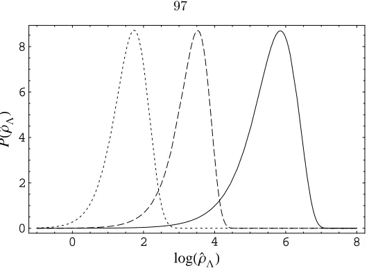
The only environmental condition that seems important to our existence and is determined in part by the cosmological constant is the existence of non-linear gravitational structures. This is described above. To account for this quantitatively it is convenient to work within the Press-Schechter formalism [37]. In this picture, one looks at the probability for a randomly selected co-moving volume to have separated from the Hubble flow by some specified time. We are interested in whether non-linear structures ever form, so we take this time to be the infinite future. Whether a given volume ever separates from the Hubble flow is a function of the mass over-densityzcontained in that volume, calculated assuming linear density perturbation evolution, and evaluated at the infinite future. The quantityz is a Gaussian random variable root-mean-square amplitude σ∞(ρΛ, µ) that
depends on both the energy density in cosmological cosntantρΛand the size of the enclosed volume,
which we parameterize by the massµthat the volume encloses. Meanwhile, for a volume to seperate from the Hubble flow requires z&1.69. Thus the likelihood that a volume enclosing at least mass µwill separate from the cosmic expansion is
F(ρΛ, µ) =
r
2 π
1 σ∞
Z ∞
1.69
exp
−12 z
2
σ2
∞
dz= erfc
1.69
√
2σ∞
, (1.31)
where clearly erfc denotes the complementary error function, erfc(x)≡2π−1/2R∞
x e−z
2 dz.
An overdensity that seperates from the Hubble flow will eventually collapse and virialize. The percentage of over-densities that eventually virialize is a function of the enclosed massµbecause the root-mean-square amplitude of the initial density perturbations depends onµ. Whether a viralized over-density will collapse into a galaxy habitable to observers like us will depend onµ, but not on the cosmological constant. Usually it is assumed that there is some minimum over-density massµ0
which will form a habitable galaxy and all larger over-densities are equally suitable for life. Then if only the cosmological constant scans over the landscape, the number of observers in a given universe will be proportional to the mass fraction in suitable galaxies in that universe, which is proportional toF. Under this reasoningF(ρΛ, µ0) gives the likelihood to for a value of the cosmological constant
ρΛ to be measured. Ifµ0is chosen to coincide with the mass of the Milky Way galaxy, then about
5% of observers measure a value of the cosmological constant smaller than the value we measure. The above explanation for the size of the cosmological constant is certainly tenuous. For one, it is inappropriate to assume that conditions appropriate for life are independent of µ aside from a cut-off at the Milky Way mass. Allowing for smaller galaxies will make the value ofρΛ that we
Any parameter on which σ∞ depends will affect the distribution ofρΛ if it too is allowed to scan.
One such possibility involves the scanning of the apparent Planck mass over meta-stable states in the fundamental theory. The apparent Planck mass may determine the abundance of baryons and dark matter, in addition to the amplitude of primordial density perturbations. Both of these quantities enter intoσ∞. Exploring this possibility is one of the subjects of Chapter 5.
Although the landscape explanation for the cosmological constant is tenuous, it must be admitted that it is among the most plausible explanations for the observation of dark energy. This, and that an enormous landscape appears to be a natural consequence of string theory, has motivated the investigation of other consequences of a landscape. One example is the study of how inflationary parameters may be selected within the multiverse, which led to the discovery of the so-called runaway inflation problem that is described and extended in Chapter 5 of this thesis. A second example is the subject of Chapter 6 of this thesis. This is the possibility that the flavor structure of the Standard Model might be discribed simply as random selection from the string theory landscape. We now provide some very brief background to this idea.
The paradigm of flavor in the Standard Model of particle physics involves the observed patterns among the elements of the coupling matrices to the following interactions:
Lflavor=λuiju¯iq j Lh+λ
d ijd¯iq
j Lh∗+λ
e ije¯il
j Lh∗+
Cij
M l
i Ll
j
Lh h , (1.32)
whereqL, lL (u, d, e) are the left (right) handed quark and lepton fields,his the Higgs, the indices
iand j label generation and we have suppressed gauge symmetry indices. To provide a theoretical description of the spectrum of flavor parameters, i.e. the observable elements of the matricesλu,d,e
and C, is a major problem for theoretical physics. Since most of these elements are very small, the historical approach has been to presume some large symmetry that is softly broken in the Standard Model [38, 39]. However, progress invoking theoretically motivated models of approximate flavor symmetry (AFS) has been limited, while the AFS program in general suffers for the extreme flexibility in its ability to explain any possible flavor patterns.
dimensions, the specific flavor patterns of the Standard Model arise statistically in a landscape ensemble where the central locations of the Standard Model particle wavefunctions are allowed to sit at independent and random positions in the extra dimensional geometry. One needs only assume that the Standard Model particle wavefunctions are highly localized (for example, having Gaussian profile) and that discrepancies between the observed spectrum of flavor parameters and the most likely landscape values are due to random selection from the full statistical ensemble. The investigation of Chapter 6 restricts attention to studying flavor in the quark sector of the Standard Model; a study of the lepton sector is in preperation at the submission time of this thesis.
Chapter 5 is based on “The scale of gravity and the cosmological constant within a landscape,” Michael L. Graesser and Michael P. Salem, arXiv:astro-ph/0611694 [41]. I initiated this project and I lead its direction. In addition, I was the first to perform all of the calculations and numerical analyses that are presented in the paper. Finally, I wrote the first draft of the manuscript and I wrote most of the subsequent editions.
Chapter 2
Infrared Regulators and SCET
II
We consider matching from SCETI, which includes ultrasoft and collinear particles, onto
SCETII with soft and collinear particles at one loop. Keeping the external fermions off their
mass shell does not regulate all IR divergences in both theories. We give a new prescription to
regulate infrared divergences in SCET. Using this regulator, we show that soft and collinear
modes in SCETIIare sufficient to reproduce all the infrared divergences of SCETI. We explain
the relationship between IR regulators and an additional mode proposed for SCETII.
Based on C. W. Bauer, M. P. Dorsten, and M. P. Salem,Phys. Rev. D 69, 114011 (2004).
2.1
Introduction
Soft-collinear effective theory [1, 2, 3, 4] describes the interactions of soft and ultrasoft (usoft) particles with collinear particles. Using light-cone coordinates in which a general four-momentum is written as pµ= (p+, p−, p⊥) = (n·p,n¯·p, p⊥), wheren and ¯n are four-vectors on the light cone (n2 = ¯n2 = 0,n
·n¯ = 2), these three degrees of freedom are distinguished by the scaling of their momenta:
collinear: pµ
c ∼Q(λ2,1, λ),
soft: pµ
s ∼Q(λ, λ, λ),
usoft: pµ
us∼Q(λ2, λ2, λ2).
(2.1)
The size of the expansion parameter λ is determined by the typical off-shellness of the collinear particles in a given problem. For example, in inclusive decays one typically has p2
c ∼ Q2λ2 ∼
QΛQCD, from which it follows that λ = pΛQCD/Q. For exclusive decays, however, one needs
collinear particles withp2c ∼Λ2QCD, givingλ= ΛQCD/Q. One is usually interested in describing the
interactions of these collinear degrees of freedom with non-perturbative degrees of freedom at rest, which satisfypµ
∼(ΛQCD,ΛQCD,ΛQCD). Thus inclusive processes involve interactions of collinear
while the latter theory is called SCETII [5].
Interactions between usoft and collinear degrees of freedom are contained in the leading-order Lagrangian of SCETI,
LI= ¯ξn
in·D+iD/⊥c
1 i¯n·DciD/
⊥
c
n/¯
2ξn, (2.2)
and are well understood. The only interaction between collinear fermions and usoft gluons is from the derivative
iDµ =iDµc +gAµus. (2.3)
These interactions can be removed from the leading-order Lagrangian by the field redefinition [4]
ξn =Ynξ(0)n , An=YnA(0)n Yn†, Yn(x) = P exp
ig
Z 0
−∞
ds n·Aus(x+ns)
. (2.4)
However, the same field redefinition has to be performed on the external operators in a given problem, and this reproduces the interactions with the usoft degrees of freedom. Consider for example the heavy-light current, which in SCETI is given by
JhlI(ω) =
¯
ξnWnωΓhv, (2.5)
where hv is the standard field of heavy quark effective theory [7], the Wilson line Wn is required
to ensure collinear gauge invariance [3], andω is the large momentum label of the gauge invariant [ ¯ξnWn] collinear system. Written in terms of the redefined fields, this current is
JhlI(ω) =
h
¯ ξn(0)Wn(0)
i
ωΓ
Yn†hv . (2.6)
For exclusive decays, we need to describe the interactions of soft with collinear particles. This theory is called SCETII [5]. Since adding a soft momentum to a collinear particle takes this particle
off its mass shell (pc+ps)2 ∼ (Qλ, Q, Qλ)2 ∼ Q2λ ∼ QΛQCD, there are no couplings of soft to
collinear particles in the leading-order Lagrangian.1 Thus, the Lagrangian is given by [6, 43, 44]
LII= ¯ξn
in·Dc+iD/⊥c
1 i¯n·DciD/
⊥
c
¯ n/
2ξn. (2.7)
In this theory, the heavy-light current is given by
JhlII(ω, κ) =
h
¯ ξn(0)Wn(0)
i
ωΓ
Sn†hvκ , (2.8)
whereSn is a soft Wilson line in thendirection defined by
Sn(x) = P exp
ig
Z 0
−∞
ds n·As(x+ns)
. (2.9)
This is the most general current invariant under collinear and soft gauge transformations.
This chapter is organized as follows: We first consider the matching of the heavy-light current in SCETI onto the heavy-light current in SCETII using off-shell fermions. While the terms logarithmic
in the off-shellness do not agree in the two theories, we argue that this is due to unregulated IR divergences in SCETII. We then discuss IR regulators in SCET in more detail. We first identify the
problems with SCET regulators and then propose a new regulator that addresses these issues. Using this regulator we then show that soft and collinear modes in SCETII are sufficient to reproduce the
IR divergences of SCETI and explain the relationship between IR regulators and an additional mode
proposed for SCETII [43, 44].
2.2
Matching from
SCET
Ionto
SCET
IIThe only difference between SCETI and SCETII is the typical off-shellness of the collinear degrees of
freedom in the theory. The theory SCETI allows fluctuations around the classical momentum with
p2
c∼QΛQCD, while the theory SCETII allows fluctuations with onlyp2c ∼Λ2QCD. Since both theories
expand around the same limit, SCETIIcan be viewed as a low energy effective theory of SCETI.
Therefore, one can match from the theory SCETI onto SCETII by integrating out theO(pQΛQCD)
fluctuations.
To illustrate this matching, we consider the heavy-light current. Using the definitions of this current given in Eqs. (2.5) and (2.8), we can write
JI hl(ω) =
Z
dκ C(ω, κ)JII
hl(ω, κ). (2.10)
At tree level one finds trivially C(ω, κ) = 1. In fact, this Wilson coefficient remains unity to all orders in perturbation theory, as was argued in Ref. [45].
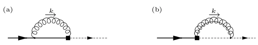
To determine the matching coefficient at one loop, we calculate matrix elements of the current in the two theories. There are two diagrams in SCETI, shown in Fig. 2.1. We use SCETI without
performing the field redefinitions of Eq. (2.4) so that the matching between SCETI and SCETII is
not trivial. For on-shell external states, we find for the two integrals
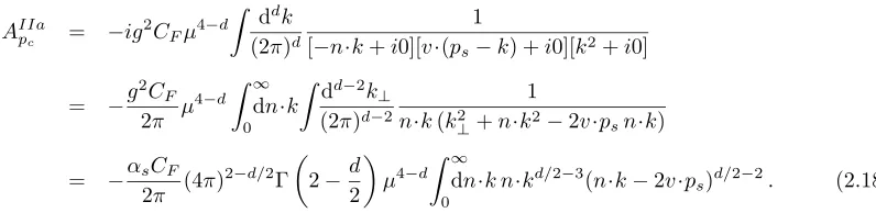
iAIa = g2CFµ4−d
Z ddk
(2π)d
1
[−n·k+i0][−v·k+i0][k2+i0], (2.11)
iAIb = 2g2CFµ4−d
Z ddk
(2π)d
¯
n·(pc−k)
[−¯n·k+i0][k2−2p
k
(a)
→
(b)
→
k
Figure 2.1: Diagrams in SCETI contributing to the matching. The solid square denotes an insertion
of the heavy-light current.
→
k
(a)
→
k
(b)
Figure 2.2: Diagrams in SCETIIcontributing to the matching.
The factor of 1/[−¯n·k+i0] in iAIb comes from the Wilson line that appears in the heavy-light
current. Meanwhile, the diagrams in SCETII are shown in Fig. 2.2. For on-shell external states the
two integrals are exactly the same as in SCETI:
iAIIa = g2CFµ4−d
Z ddk
(2π)d
1
[−n·k+i0][−v·k+i0][k2+i0], (2.13)
iAIIb = 2g2CFµ4−d
Z ddk
(2π)d
¯
n·(pc−k)
[−¯n·k+i0][k2−2p
c·k+i0][k2+i0]
. (2.14)
Since the integrands are exactly the same, the loop diagrams will precisely cancel in the matching calculation. Thus we find that the Wilson coefficientC(ω, κ) remains unity, even at one loop. This confirms the arguments in Ref. [45] to this order.
The fact that both of these integrals are scaleless and therefore that they integrate to zero might bother some readers. The vanishing of these diagrams is due to the cancellation of collinear, infrared (IR) and ultraviolet (UV) divergences. Introducing an IR regulator will separate these divergences, and the UV will be regulated by dimensional regularization. In Ref. [1] a small off-shellness was introduced to regulate the IR divergences of SCETI. In Refs. [43, 44] the divergence structure
of SCETII was studied keeping both the heavy and the collinear fermions off-shell. Using this IR
regulator, the authors of Refs. [43, 44] argued that SCETIIdoes not reproduce the IR divergences of
SCETI and introduced a new mode in SCETII to fix this problem. To gain more insight into their
In SCETI the first diagram is
AIapc = −ig
2C
Fµ4−d
Z ddk
(2π)d
1
[˜pc−n·k+i0][v·(ps−k) +i0][k2+i0]
= −g
2C
F
2π (4π)
1−d/2Γ
2−d 2
µ4−d
Z ∞
0
dn·k(n·k−p˜c)−1n·kd/2−2(n·k−2v·ps)d/2−2
= αsCF 4π
−12 +
2 log
−p˜c
µ −2 log
2−p˜c
µ + 2 log
1−2v·ps ˜ pc
log2v·ps ˜ pc
+ 2 Li2
2v·ps
˜ pc −3π 2 4 , (2.15)
where d= 4−2 and ˜pc =pc2/n¯·pc. In going from the first line to the second, we closed the ¯n·k
contour below, thus restrictingn·kto positive values, and performed the Euclideank⊥integral. The second diagram gives
AIb
pc = −2ig
2C
Fµ4−d
Z ddk
(2π)d
¯
n·(pc−k)
[−n¯·k+i0][(k−pc)2+i0][k2+i0]
= αsCF 4π 2 2 + 2 − 2 log
−p2
c
µ2 + log 2−p2c
µ2 −2 log
−p2
c
µ2 + 4−
π2
6
. (2.16)
In this diagram it is necessary to choosed <4 for the k⊥ integral, but one requires d >4 for the ¯
n·kintegral. In the former integral, dimensional regularization regulates the divergence atk⊥=∞, while in the latter it regulates the divergence at ¯n·k = 0. Both of these divergences have to be interpreted as UV, as discussed in Section 2.3. In addition, each of the diagrams contains a mixed UV-IR divergence of the form logp2c/. This mixed divergence cancels in the sum of the two diagrams
and we find, after also adding the wave function contributions,
AIpc =
αsCF
4π 1 2 + 2 log µ ¯ n·pc
+ 5 2+ log
2−p2c
µ2 −2 log 2−p˜c
µ − 3 2log
−p2
c
µ2 −2 log
−2v·ps
µ
+ 2 log
1−2v·ps ˜ pc
log2v·ps ˜ pc
+ 2Li2
2v ·ps
˜ pc +11 2 − 11π2 12 . (2.17)
This reproduces the IR behavior of full QCD.
Now consider the SCETII diagrams. The second is identical to the one in SCETI: AIIbpc =A
Ib pc.
k
→
The first diagram, however, is different. For this amplitude we find
AIIa
pc = −ig
2C
Fµ4−d
Z ddk
(2π)d
1
[−n·k+i0][v·(ps−k) +i0][k2+i0]
= −g
2C
F
2π µ
4−dZ ∞
0
dn·k
Z dd−2k
⊥ (2π)d−2
1 n·k(k2
⊥+n·k2−2v·psn·k)
= −αsCF 2π (4π)
2−d/2Γ
2−d 2
µ4−d
Z ∞
0
dn·k n·kd/2−3(n·k−2v·ps)d/2−2. (2.18)
Note that convergence of this integral at n·k=∞requiresd <4, whereas convergence atn·k= 0 requiresd >4. Here dimensional regulation is regulating both a UV divergence atn·k=∞, as well as the divergence at n·k = 0 , which is IR in nature, as we will discuss in Section 2.3. Using the variable transformationx=n·k/(n·k−2v·ps) to relate this integral to a beta function [46] one finds
AIIapc =
αsCF
4π 1 2− 2 log
−2v·ps
µ + 2 log
2−2v·ps
µ + 5π2
12
. (2.19)
Adding the two diagrams together with the wave function contributions gives αsCF
4π 3 2 − 2 log
2v·psp2c
µ3 +
5 2+ log
2−p2c
µ2 + 2 log
2−2v·ps
µ − 3 2log
−p2
c
µ2
−2 log−2v·ps µ + 11 2 + π2 4 . (2.20)
We can see that in the sum of the two diagrams the terms proportional to logp2
c/or logv·ps/do
not cancel as they did in SCETI. Furthermore, the finite terms logarithmic inp2c orv·psdo not agree
with the corresponding terms in the SCETI result. This fact prompted the authors of Refs. [43, 44]
to conclude that SCETII does not reproduce the IR divergences of SCETII and that a new mode is
needed in the latter effective theory. However, as we mentioned above, there are problems with IR effects in this diagram. In fact, as we will show in great detail in the next section, the off-shellness of the fermions does not regulate all IR divergences in this diagram. This means that the fact that the terms logarithmic in the fermion off-shellness do not agree between SCETI and SCETII does not
imply that the IR divergences are not reproduced correctly since some 1/poles are IR in origin. We also calculate the diagram in SCETII containing the additional mode proposed in Refs. [43,
44]. The new messenger mode has momenta scaling pµ
sc ∼(Λ2QCD/Q,ΛQCD,Λ3QCD/2 /Q1/2). (Note
that the invariant mass of this term satisfies p2
sc ∼Λ3QCD/Q Λ2QCD.) The diagram is shown in
Fig. 2.3 and for its amplitude we find
AIIcpc = −2ig
2C
Fµ4−d
Z ddk
(2π)d
1
[˜pc−n·k+i0][2v·ps−n¯·k+i0][k2+i0]
= αsCF 4π
−22 +
2 log
2v·psp˜c
µ2 −log
22v·psp˜c
µ2 −
π2
2
Adding this term to the Eq. (2.20) cancels the terms proportional to log(2v·psp2c/µ3)/and we find
AIIpc =
αsCF
4π
1 2 +
2 log
µ ¯ n·pc
+ 5 2+ log
2−p2c
µ2 −
3 2log
−p2
c
µ2 −2 log
−2v·ps
µ
+ 2 log2
−2v·ps
µ
−log2
2v ·psp˜c
µ2
+11 2 −
π2
4
. (2.22)
This result does not agree with the SCETI expression in Eq. (2.17). However, this is expected, since
the off-shellness in SCETIIsatisfies ˜pc v·ps. In this limit the SCETI result in Eq. (2.17) agrees
with the result in Eq. (2.22).
2.3
Infrared Regulators in SCET
2.3.1
Problems with Known IR Regulators
One of the most important properties of SCETI is the field redefinition given in Eq. (2.4), which
decouples the usoft from the collinear fermions. It is the crucial ingredient for proving factorization theorems. Furthermore, only after performing this field redefinition is it simple to match from SCETI onto SCETII, since one can identify the Wilson line Yn in SCETI with the Wilson line
Sn in SCETII. However, it is a well known fact that field redefinitions only leave on-shell Green
functions invariant [47]. Hence, the off-shellness of the collinear quark p2c used to regulate the IR
in SCETI takes away our ability to perform this field redefinition. Since no field redefinition is
performed on the heavy quark, one is free to give it an off-shellness.
IR divergences appear in individual diagrams, but they cancel in the set of diagrams contributing to a physical observable. More specifically, the IR divergences in virtual loop diagrams are cancelled against those in real emissions, which physically have to be included due to finite detector resolutions. From this it is obvious that the IR divergences in the heavy-light current originate from regions of phase space where either the gluon three-momentum |k|or the angleθ between the gluon and the light fermion goes to zero. Other divergences arise if the three-momentum of the gluon goes to infinity orθgoes toπ. These divergences are UV. To check if the IR divergences match between the two theories one has to use an IR regulator that regulates all IR divergences in both theories. To get insight into the behavior of the three-momentum and the angle, it will be instructive to perform the required loop integrals by integrating overk0using the method of residues, and then integrating over
in the SCETI one-loop calculation of the previous section are UV. For the first diagram we find
AIapc = −ig
2C
Fµ4−d
Z ddk
(2π)d
1
[˜pc−n·k+i0][v·(ps−k) +i0][k2+i0]
= −g
2C
F
2
Ωd−2
(2π)d−1µ 4−dZ ∞
0
d|k||k|d−2 Z 1
−1
dcosθsind−4θ
(|k|(1−cosθ)−p˜c) (|k| −v·ps)|k|
. (2.23)
Performing the remaining integrals, we of course reproduce the result obtained previously, but this form demonstrates that all divergences from regions |k| →0 and (1−cosθ)→0 are regulated by the infrared regulators and thus all 1/divergences are truly UV.
The second diagram is
AIbpc = −2ig
2C
Fµ4−d
Z ddk
(2π)d
¯
n·(pc−k)
[−n¯·k+i0][(pc−k)2+i0][k2+i0]
= −2ig2C
F[I1+I2], (2.24)
where I1 and I2 are the integrals with the ¯n·pand the ¯n·k terms in the numerator, respectively.
The integralI2is standard and we find
I2= i
16π2
1 −log
−p2
c
µ2 + 2
, (2.25)
where regulates only UV divergences. For the first integral we again perform thek0 integral by
contours and we find
I1 =
i¯n·pc
2
Ωd−2
(2π)d−1µ 4−dZ ∞
0
d|k||k|d−2 Z 1
−1
dcosθsind−4θ
× "
−k2(1 + cosθ)[2|k|(p1
0− |p|cosθ)−p2c]
+ 1
a[p0+a+|k|cosθ][2p20+ 2p0a−2|k||p|cosθ−p2c]
#
, (2.26)
wherepc = (p0,p) anda=
p
k2+p2−2|k||p|cosθ. From this expression we can again see that all
IR singularities from|k| →0 and (1−cosθ)→0 are regulated by the off-shellness, and all remaining divergences are UV. Note furthermore that in the limit|k| → ∞, with unrestrictedθ, the two terms cancel each other, so that there is no usual UV divergence. This agrees with the fact that there are five powers ofk in the denominator of the integrand in Eq. (2.24). However, in the limit|k| → ∞
with|k|(1 + cosθ)→0 the second term of Eq. (2.26) remains finite, whereas the first term develops a double divergence. Thus, it is this region of phase space that gives rise to the double pole in this diagram. The presence of the square roots makes the evaluation of the remaining integrals difficult, but we have checked that we reproduce the divergent terms of the result given in Eq. (2.16).
the IR divergences, and that the 1/ divergences all correspond to divergences of UV origin. The situation is different in SCETII, since the off-shellness of the light quark does not enter diagram (a).
In this case we find
AIIapc = −ig
2C
Fµ4−d
Z ddk
(2π)d
1
[−n·k+i0][v·(ps−k) +i0][k2+i0]
= −g
2C
F
2
Ωd−2
(2π)d−1µ 4−dZ ∞
0
d|k||k|d−2 Z 1
−1
dcosθ sind−4θ
k2(1−cosθ)(|k| −v·p
s)
. (2.27)
The IR divergence originating from the limit (1−cosθ)→0 is not regulated by the off-shellness. Thus part of the 1/divergences in Eq. (2.19) are of IR origin. In other words, the fact that the terms logarithmic in the off-shellness in the SCETI amplitude Eq. (2.17) are not reproducing the
corresponding terms in the SCETIIamplitude Eq. (2.20) does not imply that the IR divergences
do not match between the two theories. In order to check whether the IR divergences of the two theories match, one needs a regulator that regulates all IR divergences in both SCETI and SCETII.
As an alternative IR regulator one could try to use a small gluon mass. Consider the first diagram in SCETI again, this time with a gluon mass. We find
AIam = −ig2CFµ4−d
Z ddk
(2π)d
1
[−n·k+i0][v·(ps−k) +i0][k2−m2+i0]
= −g
2C
F
2
Ωd−2
(2π)d−1µ 4−dZ ∞
0
d|k||k|d−2 Z 1
−1
dcosθsind−4θ
× 1
(k2+m2−v·p
s
√
k2+m2)(√k2+m2− |k|cosθ). (2.28)
Again, all divergences|k| →0 and (1−cosθ)→0 are regulated b
![Figure 2.3: Contribution of the additional SCETII mode proposed in Refs. [43, 44].](https://thumb-us.123doks.com/thumbv2/123dok_us/1127940.1141605/31.612.125.536.96.212/figure-contribution-additional-scetii-mode-proposed-refs.webp)