Volume 2010, Article ID 641842,14pages doi:10.1155/2010/641842
Research Article
Noiseless Codelength in Wavelet Denoising
Soosan Beheshti, Azadeh Fakhrzadeh, and Sridhar Krishnan
Department of Electrical and Computer Engineering, Ryerson University, Toronto, ON, Canada M5B 2K3
Correspondence should be addressed to Soosan Beheshti,[email protected]
Received 27 April 2009; Revised 14 October 2009; Accepted 4 January 2010
Academic Editor: Christoph Mecklenbr¨auker
Copyright © 2010 Soosan Beheshti et al. This is an open access article distributed under the Creative Commons Attribution License, which permits unrestricted use, distribution, and reproduction in any medium, provided the original work is properly cited.
We propose an adaptive, data-driven thresholding method based on a recently developed idea of Minimum Noiseless Description Length (MNDL). MNDL Subspace Selection (MNDL-SS) is a novel method of selecting an optimal subspace among the competing subspaces of the transformed noisy data. Here we extend the application of MNDL-SS for thresholding purposes. The approach searches for the optimum threshold for the data coefficients in an orthonormal basis. It is shown that the optimum threshold can be extracted from the noisy coefficients themselves. While the additive noise in the available data is assumed to be independent, the main challenge in MNDL thresholding is caused by the dependence of the additive noise in the sorted coefficients. The approach provides new hard and soft thresholds. Simulation results are presented for orthonormal wavelet transforms. While the method is comparable with the existing thresholding methods and in some cases outperforms them, the main advantage of the new approach is that it provides not only the optimum threshold but also an estimate of the associated mean-square error (MSE) for that threshold simultaneously.
1. Introduction
We can recognize different phenomena by collecting data from them. However, defective instruments, problems with the data acquisition process, and the interference of natural factors can all degrade the data of interest. Furthermore, noise can be introduced by transmission errors or compres-sion. Thus, denoising is often a necessary step in data pro-cessing and various approaches have been introduced for this purpose. Some of these methods, such as Wiener filters, are grouped as linear techniques. While these techniques are easy to implement, their results are not always satisfactory. Over past decades, researchers have improved the performance of denoising methods by developing nonlinear approaches such as [1–6]. Although these approaches have succeeded in providing better results, they are usually computationally exhaustive, hard to implement, or use particular assumptions either on the noisy data or on the class of the data estimator. Thresholding methods are alternative approaches to the denoising problem. The thresholding problem is first formulated in [7] where VisuShrink is introduced. This threshold is a nonadaptive universal threshold and depends
only on the number of data points and noise variance. VisuShrink is a wavelet thresholding method which is both simple and effective in comparison with other denoising techniques. When an orthogonal wavelet basis is used, the coefficients with small absolute values tend to be attributed to the additive noise. Taking advantage of this property, finding a proper threshold, and setting all absolute values of coefficients smaller than the threshold to zero can suppress the noise. The main issue in such approaches is to find a proper threshold. In using the thresholding method for image denoising, the visual quality of the image is of great concern. An improper threshold may introduce artifacts and cause blurring of the image. One of the first soft thresholding methods is SureShrink [8] which has a better effect on the image than Visushrink in many cases. This method uses a hybrid of the universal threshold and the SURE (Stein’s Unbiased Risk Estimator) threshold. The SURE threshold is chosen by minimizing Stein’s estimate.
process, in this case reconstructing the denoised signal from the noisy one, the major goal is to achieve the original signal as much as possible, and the MSE is one of the most used criteria for evaluation purposes. To find the optimum threshold we estimate the MSE of a set of completing thresholds and choose the one that minimizes this error. The fundamentals of MSE estimation are similar to the method proposed in Minimum Noiseless Description Length (Codelength) Subspace Selection (MNDL-SS) [10]. Each subspace in this approach keeps a subset of the coefficients and discards the rest. Thresholding also produces a subspace that includes a set of coefficients that are being kept. On the other hand, it was shown in [10] that an estimate of noiseless description length (NDL) can be provided for each subspace by using the noisy data itself. We also show that in the process of estimating the NDL, the estimates of MSE is also provided. Furthermore comparison of the NDL of com-peting subspaces is equivalent to comparison of their MSEs. Therefore, the method presented in this paper is denoted by MNDL thresholding. The competing thresholds that are the sorted coefficients generate competing subspaces. For these subspaces the estimate of MSEs are provided and compared. The optimum threshold is associated with the subspace with minimum MSE (equivalently minimum NDL). Because of the particular choice of competing subspaces in MNDL thresholding, the effect of the additive noise is different from that in MNDL-SS. While the independence of the additive noise in MNDL-SS is the main advantage in estimating the desired NDL, in the case of thresholding, the additive noise is highly dependent. The main challenge in this work is to develop a method for NDL estimation acknowledging the presence of this noise dependence. We provide a threshold that is a function of the noise varianceσ2
w, the data lengthN, and the observed noisy data itself.
The paper is arranged as follows.Section 2describes the considered thresholding problem.Section 3briefly describes the fundamentals of the existing MNDL subspace selection. Section 4 introduces the MNDL thresholding approach. Hard and soft MNDL thresholdings are presented in Sections 5 and 6. Section 7 provides the simulation results and Section 8is our conclusion.
2. Problem Statement
Noiseless data {y(i), i = 1,. . .,N} of length N has been corrupted by an additive noise:
y(i)=y(i) +w(i), (1)
where w(i) is an independent and identically distributed (i.i.d) Gaussian random process with zero mean and variance
σ2
w. ( The method presented here is for real data. However, it can also be used for complex data. ) In the considered denoising process, we project the noisy data into an orthog-onal basis. The goal is to provide the optimum threshold for the resulting coefficients that minimizes the mean square error.
Assume that the noiseless data vector yN = [y(1) y(2)
· · ·y(N)]T is generated by space SN. The spaceSN can be expanded by orthogonal basis vectors:
si,sj
=
⎧ ⎨ ⎩
1 ifi=j,
0 ifi /=j, (2)
wheresi,sjis the inner product of vectorssiandsj. The data in (1) is represented in this basis as follows:
yN = N
i=1
θ(i)si, yN = N
i=1
θ(i)si, wN = N
i=1
v(i)si,
(3)
θ(i)=θ(i) +v(i), (4)
where θ(i) is the ith coefficient of the noiseless data, θ(i) is thei-th coefficient of the noisy data, andv(i) is thei-th coefficient of the additive noise. Note that since the basis vectors ofSNare orthogonal,v(i) is also a sample of Gaussian distribution with zero mean and variance,σ2
w.
The thresholding approach uses the available noisy coefficients,θ, to provide the best estimate of the noiseless coefficients denoted byθ. There are two general thresholding methods: hard and soft thresholdings. Hard thresholding eliminates or keeps the coefficients by comparing them with the threshold
θ(i)=
⎧ ⎨ ⎩
θ(i), if|θ(i)| ≥Th,
0, otherwise, (5)
whereThis the hard threshold. Soft thresholding eliminates the coefficients below Tsand reduces the absolute value of the rest of the coefficients:
θ(i)=
⎧ ⎨ ⎩
sgn(θ(i))(|θ(i)| −Ts), if|θ(i)| ≥Ts,
0, otherwise. (6)
There are different approaches for calculation of the proper
Th andTs. In this paper, we expand the existing theory of the MNDL subspace selection method in [10] to provide new hard and soft thresholding methods.
Important Notation. In this paper a random variable is denoted by a capital letter, such asWandV, while a sample of that random variable is represented by the same letter in lower case such aswandv.
3. MNDL Subspace Selection (MNDL-SS)
data in that subset and sets the rest of the coefficients to zero. Among competing subspaces, MNDL-SS chooses the subspace that minimizes the description length (codelength) of “noiseless” data. In this setting subspaces of the spaceSN are chosen as follows: Each Sm is a subspace of SN that is spanned by the firstmelements of the bases. The estimate of the noiseless coefficients in subspaceSmis
θSm(i)=
⎧ ⎨ ⎩
θ(i), ifsi∈Sm,
0, otherwise, (7)
and the estimate of the noiseless data inSm,yNSm, is
yNSm=
N
i=1
θsm(i)si. (8)
In each subspace the description length (codelength) of the noiseless data is defined as [10] ( this criterion is different from MDL criterion and the explanation is provided in [10])
DL yN;yNSm
=log2
2πσ2 w+
log2e
2σ2 w
zSm, (9)
where zSm is the reconstruction error ( the equality of the
error in the time domain and the error in coefficients of data is the result of the Parseval’s Theorem) :
zSm =
1
N yN−yN
Sm 2 2= 1 N θN−θN
Sm 2
2
, (10)
which is a sample of random variableZSm.
The optimum subspace Smopt can be chosen by
min-imizing the average description length of noiseless data among the competing subspaces. Minimizing the average of noiseless data length in (9) is equivalent to minimizing the mean square error (MSE) in the form ofE(ZSm) as the term
log22πσ2
wis a constant and not a function ofm:
mopt=arg min Sm
EZSm
. (11)
MNDL-SS estimates the MSE for each subspace by using the available data errorxSm in that subspace. The data error is
defined in the following form:
xSm=
1
N
yN−ySNm 2 2= 1 N θN−θN
Sm 2
2, (12)
which is a sample of random variableXSm. MNDL-SS studies
the structure of the two random variablesZSm andXSm and
uses the connection between these two random variables to provide an estimate of the desired criterion E(ZSm) for
differentm.
4. MNDL Thresholding
To use the ideas of subspace selection in thresholding, we first have to explain how a particular choice of subspaces serves the problem of thresholding. In MNDL-SS, the competing subspaces are chosen a priori and are not functions of the
observed data. However, if the method is going to be used for thresholding, forming the competing subspaces is based on the observed data. In this case, we first sort the bases based on the absolute value of the observed noisy coefficientsθ. This will dictate a particular indexing on the bases such that
|θ(1)| ≥ |θ(2)| ≥ · · · ≥ |θ(N)|. (13)
Therefore, the first subset represents the basis associated with the largest absolute value of the coefficients. The subset with two coefficients includes the two bases with the largest absolute value of the sorted coefficients and so on. The subspaceSmincludesmof the basis and represents the first
mlargest absolute values of the coefficients and as a result this subspace represents thresholding with a threshold value ofθ(m).
Back to the MNDL-SS, the subspaceSmoptthat minimizes
the average codelength of the noiseless data (equivalent to the subspace MSE in (11)) is the optimum subspace. Due to the indexing in the form of (13), the choice of this subspace results in the optimum thresholdθ(mopt).
To estimate the MSE of the subspaces, we follow the fundamentals of the MNDL-SS method. Due to the random choice of subspaces in MNDL-SS, the random variablesV(i)s that represent the additive noise of the coefficients in (4) are independentGaussian random variables. In MNDL thresh-olding, the additive noise of coefficients is still Gaussian. However, due to the particular choice of the index for the coefficients,V(i)s are no longer independent. This will cause a major challenge in estimating the MSE of subspaces and is the main focus of this paper.
5. MNDL Hard Thresholding
In [10] it is shown that the expected value of the reconstruc-tion error and that of the data error in subspaceSm can be written in the form of
EZSm
=EAZsm
+ 1
NΔSm
2
2, (14)
EXSm
=EAXsm
+ 1
NΔSm
2
2, (15)
where ΔSm2 is the l2-norm of the discarded coefficient vector in subspaceSm:
1
NΔSm
2 2= 1 N N
i=m+1
θ2(i), (16)
and the noise parts are
EAZsm
= 1 N
m
i=1
E V(i)2, (17)
EAXsm
= 1 N
N
i=m+1
E V(i)2, (18)
θm
+1
θm
+1 θm
θm − 1 θm − 1
Figure1: Distributions ofθ(m+ 1),θ(m), andθ(m−1).
If the noise partsE(AZsm) andE(AXsm) are available, then
by estimating the expected value of the data error with the available samplexSmwe have
1
NΔSm
2
2≈xSm−E
AXsm
. (19)
and then the estimate of the desired MSE in (14) is
EZSm
≈xSm−E
AXsm
+EAZsm
. (20)
The main challenge in MNDL thresholding is in calculating
E(AXsm) and E(AZsm) in (18) and (17). In MNDL-SS, due
to the independence ofV(i)s in (4), random variablesAXsm
andAZsm are Chi-square random variables and calculation
of the expected values of these terms is straight forward. However, in MDNL thresholding, since the V(i)s are not independent, calculation of these expected values is not easy. In the following section we focus on estimating these desired expected values for the case of thresholding.
5.1. Estimate of MSE in MNDL Hard Thresholding. In order to calculate the expected value of the additive noise in (17) and (18), we need to study the noise effects that are associated with the sorted noisy coefficients. Each θ(i) in (4) has a Gaussian distribution with meanθ(i) and variance
σ2
w.Figure 1shows the distribution of θ(m+ 1),θ(m), and
θ(m−1). The expected value of the noise part ofθ(m) under the conditionθ(m+ 1)< θ(m)< θ(m−1) is as follows:
EV2(m)=σ2
w+εh(d1(m),d2(m)), (21) where
d1(m)=θ(m+ 1)−θ(m), (22)
d2(m)=θ(m−1)−θ(m), (23)
andεh(d1(m),d2(m)) is
εh(d1(m),d2(m))= f1
(m)−f2(m)
Q(d1(m))−Q(d2(m))
, (24)
whereQ(x)=1/2π∞x exp(−t2/2)dtandf1(m) andf2(m) are defined as
f1(m)= √σw 2πd1(m)e
−d2
1(m)/2σw2, (25)
f2(m)= √σw
2πd2(m)e
−d2
2(m)/2σw2. (26)
Details of the calculationare provided inAppendix B.
Therefore, for the desired noise parts we have
E nzSm
= 1 N
m
i=1
EV2(i) (27)
=m Nσ 2 w+ 1 N m
i=1
εh(d1(i),d2(i)). (28)
Similarly we have
E nxSm
= 1 N
N
i=m+1
EV2(i) (29)
=N−(m+ 1)
N σ 2 w+ 1 N N
i=m+1
εh(d1(i),d2(i)).
(30)
The noise part of the MSE in (27) and the noise part of the expected value of data error in (29) are dependent ond1,d2 that are not available. We suggest estimating them by using the available data as follows [11].
(i) Generate gi Gaussian vectors of data length with variance of the additive noise.
(ii) Sort the absolute value of the associated noise coefficients,gsort
i .
(iii) Find the estimate of the expected value of this vector
E[Gsort] by averaging over 50 samples of these vectors:
EGsort(m)≈ 1 50
50
i=1
gsort
i (m). (31)
(iv) Estimateθas follows:
θ(m)=θ(m)−EGsort(m). (32)
(i) Estimated1andd2by replacingθwithθin (22) and (23):
d1(m)=θ(m+ 1)−θ(m), (33)
d2(m)=θ(m−1)−θ(m). (34)
The estimates of the noise parts in (27) and (29) are
E nzSm
=m Nσ 2 w+ 1 N m
i=1
εh d1(i),d2(i)
, (35)
E nxSm
= 1
N
N
i=m+1
εh d1(i),d2(i)
+N−(m+ 1)
N σ
2 w.
(36)
(i) Estimate the noise parts E(nxSm) and E(nzSm) using
(36) and (35).
(ii) Estimate the MSE in (20) as follows:
EZSm
=xSm−E
AXsm
+EAZsm
. (37)
In MNDL thresholding the goal is to find mopt by minimizing the MSE in (11). Here we provide an estimate ofmoptusing the MSE estimate:
mopt=arg min Sm
EZSm
, Th=θmopt. (38)
6. MNDL Soft Thresholding
In some applications, such as image denoising, soft thresh-olding generally performs better and provides a smaller MSE than hard thresholding [12]. In soft thresholding, not only are the values smaller than the threshold set to zero, but also the value of coefficients larger than the threshold is also reduced by the amount of the threshold. Thus, we need to take into account this changing level of coefficients in MSE estimation. For MNDL soft thresholding we follow the same procedure as in MNDL hard thresholding. Here, the MSE in subspaceSmis
EZsm
= 1 NE
⎛ ⎝m
i=1
(V(i)−Tm)2
⎞ ⎠+ 1
NΔSm
2
2, (39)
whereTmis the smallest coefficient in subspaceSm(which is
θm).
6.1. Noise Effects in the MSE. The noise part of the MSE in (39) is
E nzsm
= 1 N
m
i=1
E(V(i)−Tm)2, (40)
whereV(i)s are the associated noise parts of coefficientsθ(i)s in subspaceSm. The expected value of the noise part ofθ(i) under the conditionθ(i+ 1)< θ(i)< θ(i−1) is
E(V(i)−Tm)2
=Tm2 +σw2+εs(d1(i),d2(i),Tm), (41)
whered1(i) andd2(i) are defined similar to those in (22) and (23), andεs(d1(i),d2(i),Tm) is defined as
εs(d1(i),d2(i),Tm)= j1
(i,Tm) +j2(i,Tm)
Q(d1(i))−Q(d2(i))
, (42)
wherej1(i,m) andj2(i,m) are defined as
j1(i,Tm)=√σw 2πe
−d2 1(i)/2σw2(d
1(i)−2Tm), (43)
j2(i,Tm)=√σw 2πe
−d2
2(m)/2σw2(2T
m−d2(i)). (44)
Details of this calculation are provided inAppendix C.
Using the estimates ofd1andd2from (33) and (34), the estimate of MSE’s noise part in (40) is
E nzSm
=m
N
T2 m+σw2
+ 1
N
m
i=1
εsd1 (i),d2(i),Tm
. (45)
6.2. Estimate of the Noiseless Part of MSE. To complete the estimation of MSE in (39), we need also to estimate the noiseless part using the data error. The expected value of the data error in the case of soft thresholding is
EXSm
=m NTm+
1
NΔSm
2 2+ 1 N N
i=m+1
EV2(i) (46)
(Details are provided inAppendix A). The last component is the same as noise part in MNDL hard thresholding in (29) and can be estimated by using (36). Therefore, by estimating
E(XSm) with its available samplexSm, from (46) we have
1
N ΔSm
2=xSm− m NTm−
N−(m+ 1)
N σ 2 w − 1 N N
i=m+1
εh d1(i),d2(i),Tm
.
(47)
whereεhis defined in (24) andd1andd2are defined in (33) and (34).
6.3. Calculating the Threshold. The two components of MSE in (39) were estimated in previous sections. Therefore, the MSE can be estimated as follows.
(i) The noise part is estimated by using (45). (ii) The noiseless part is estimated by using (47). (iii) The estimate of the MSE in (39) is the sum of (45)
and (47):
EZSm
= 1 N ΔSm
2+EAZsm
. (48)
Similar to MNDL hard thresholding, the optimum subspace is the one for which the estimate of the MSE is minimized:
mopt=arg min Sm
EZSm
, Ts=θmopt. (49)
1000 500
0
−5
0 5 10 15
(a)
1000 500
0
−20
0 20 40 60
(b)
1000 500
0
−10
−5
0 5 10 15
(c)
1000 500
0
−20
0 20 40 60
(d)
Figure2: (a) Blocks signal with length 1024, (b) wavelet coefficients, (c) noisy blocks signal with additive white noise,σw=1, and (d) noisy coefficients.
(i) The discrete wavelet transform of the image is taken.
(ii) In every subband the MSE, in (39), is estimated as a function of theSm: the noise part is estimated using (45), and the noiseless part is estimated using (47). MSE estimateE(ZSm) is the sum of the noiseless part
and the noise part estimates.
(iii) In each subband, the MSE is minimized over values of m, and mopt in (38) is chosen, where (m ∈
{1, 2,. . .,N}), andNis the number of coefficients in the subband.
(iv) In each subband, themoptth largest absolute value of the coefficients is the optimum threshold.
(v) The image is denoised using the subband thresholds.
(vi) The inverse discrete wavelet transform is taken.
The unknown noise variance is estimated by the median estimator,σn = MAD/0.675, where MAD is the median of
absolute value of the wavelet coefficients at the finest decom-position level (the diagonal direction of decomdecom-position level one).
In the following section we provide simulation results of the method. The low complexity of this algorithm is an additional strength of the method. Our future plan is to utilize the approach for potential applications in areas such as biomedical engineering [13].
7. Simulation Results
400 300
200 100
0
−10
−5
0 5 10
(a)
400 300
200 100
0
−20
−10
0 10 20
(b)
400 300
200 100
0
−20
−10
0 10 20
(c)
400 300
200 100
0
−20
−10
0 10 20
(d)
Figure3: (a) Mishmash signal with length 1024, (b) wavelet coefficients, (c) noisy Mishmash signal with additive white noise,σw=5, and (d) noisy coefficients.
Table 1: Comparing mopt and its estimates using MNDL hard thresholding and MNDL-SS methods for the Blocks signal.
mopt mopt mopt
Optimum order Hard thresholding MNDL-SS
σw=1 72 74 91
σw=3 34 32 40
σw=5 22 19 37
[14]. The other signal is the Mishmash signal of length 1024 with no nonzero coefficients inFigure 3.
The MSE and its estimates using the existing MNDL-SS method [10] and the developed MNDL hard thresholding method are shown in Figure 4. The mopt that minimizes the unavailable MSE and its estimate, mopt, with these approaches are provided in Table 1 for different noise variances. The results in this table and the rest of the results in this section are averages of five runs. As the figure
and the table show, as was expected MNDL thresholding outperforms the MNDL-SS approach.
Table 2compares the MSE of the proposed hard thresh-olding method with that of two hard threshthresh-olding meth-ods, VisuShrink and MDL. The comparison includes the optimum hard MSE, which represents the minimum MSE when the noisy coefficients are used as hard thresholds, along with the resulting MSE of different approaches. As the table shows, in most cases, MNDL hard thresholding provides the minimum MSE among the approaches.
The MSE and its estimate with MNDL soft thresholding are shown inFigure 5. The results in this figure are for Blocks and Mishmash signals and for two different levels of the additive noise. As the figure shows, MSE estimates are very close to the MSE itself.
1000 500
0 0 10 20 30
(a)
1000 500
0 0 5 10 15
(b)
1000 500
0 0 50 100 150
(c)
1000 500
0 0 50 100 150
(d)
Figure4: Desired unavailable MSE (solid red line), and its estimate using MNDL hard thresholding (- -) and MNDL-SS (. -) as a function ofm. (a) Blocks signal withσw=1, (b) Blocks signal withσw=5, (c) Mishmash signal withσw=1, and (d) Mishmash signal withσw=5.
subband-dependent has the best results while for Mishmash MNDL soft thresholding outperforms the other approaches in almost all cases. While here we have shown the simulation results for two of six test signals in [8], the results for the other two signals (Heavy sine, Doppler) are similar to those of the provided signals.
7.1. Image Denoising. There are many image denoising approaches, such as recent work in [15, 16]. These approaches have succeeded in providing good results. They usually use a particular assumption either on the noisy image and/or on the class of the data estimator. A well-known image denoising thresholding approach is BayesShrink.
BayesShrink [12] is a thresholding method that is also widely used for image denoising. This method attempts to minimize the Bayes’ Risk Estimator function assuming a prior Generalized Gaussian Distribution (GGD) and thus yields a data adaptive threshold [17]. Note that our method does not make any particular assumption on the data and is not especially proposed for image denoising. Here we use the approach for images as an example of a class of two-dimensional data.
Table2: MSE comparison of different thresholding methods with the MNDL hard thresholding approach.
Blocks Optimum hard MSE MNDL-SS MNDL hard thresholding MDL VisuShrink
σw=1 0.13 0.3 0.18 0.2 0.2
σw=3 1.8 2.8 1.5 2.1 2.2
σw=6 7.9 9.3 9 9 9.2
σw=10 14 17.6 17.2 17.7 15.4
Bumps
σw=1 0.3 0.33 0.32 0.33 0.37
σw=3 1.32 1.54 1.4 1.68 1.5
σw=6 4.16 6.1 5 5.2 4.9
σw=10 9.3 11.3 10.59 15.7 10.63
Quadchirp
σw=1 0.96 1 .98 1.4 2.29
σw=3 6.62 4.7 6.75 7 6.9
σw=6 7.7 8.9 7.8 10.51 8.01
σw=10 7.86 12 7.86 15.9 8.5
Mishmash
σw=1 0.9 1.2 0.9 2 3.3
σw=3 7.1 7.8 7.5 7.4 7.3
σw=6 7.8 8 7.8 10 7.9
σw=10 7.86 8.2 7.86 16 8
1000 500
0 0 5 10 15 20
(a)
1000 500
0 0 10 20 30
(b)
1000 500
0 0 5 10
True Estimate
(c)
1000 500
0 0 10 20 30
True Estimate
(d)
Table3: MSE for (1) Optimum soft thresholding; (2) Optimum Subband-dependent soft thresholding; (3) MNDL soft thresh-olding, (4) MNDL Subband-dependent soft threshthresh-olding, (5) Sureshrink.
Blocks 1 2 3 4 5
σw=1 0.3 0.18 0.3 0.21 0.27
σw=3 2.1 1.13 2.2 1.23 1.35
σw=6 6.5 3.2 6.9 3.8 3.3
σw=10 12.1 7.9 12.5 8 9.7
Bumps
σw=1 0.3 0.23 0.3 0.26 0.3
σw=3 1.6 1.13 1.6 1.32 1.5
σw=6 4.2 3.2 4.3 3.8 3.9
σw=10 8 7.7 8.3 9.9 8.6
Quadchirp
σw=1 0.82 0.83 1 0.9 0.91
σw=3 4.5 4.7 4.6 4.8 6.5
σw=6 7.2 8.1 7.5 8.9 8.5
σw=10 7.8 13.19 9.03 15 13.5
Mishmash
σw=1 0.9 0.95 1.2 1.3 1.2
σw=3 4.8 5 4.9 5.1 7
σw=6 7.3 8.5 7.5 9.1 9
σw=10 7.7 12.7 8.8 14.5 12.8
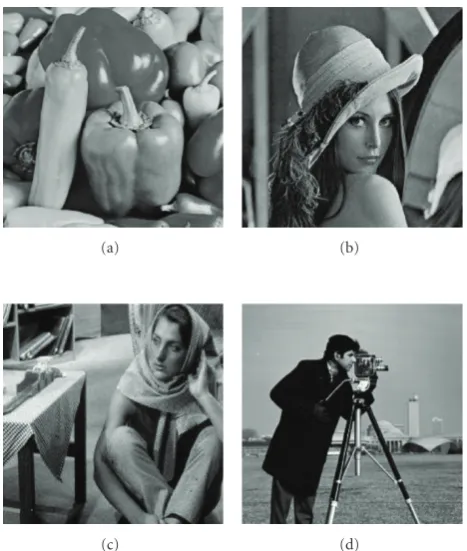
in Figure 6and with size 512×512. The wavelet transform employs Daubechies’s wavelet with eight vanishing moments and with four scales of orthogonal decomposition.
In Table 4, we compare the MSE of the MNDL with two well-known thresholding methods: BayesShrink [12] and SureShrink [8]. All these thresholds are soft subband-dependent. As the table shows, MNDL thresholding per-forms better than SureShrink in most cases and is compa-rable with the BayesShrink. The MNDL soft thresholding is compared visually with BayesShrink and SureShrink in Figure 7. As the figure shows, the ringing effect at the edges of the image with the MNDL soft thresholding is less than that with the BayesShrink approach. The importance of the new approach is that it can provide an estimate of MSE simultaneously. Note that it can also provide estimate of MSE for other thresholding methods as follows. Find the closest absolute value of the coefficients to the given threshold and use the index m of that coefficient and check the estimate of MSE for the associated Sm. Table 5 shows the optimum subband threshold for Cameraman and Table 6 shows the thresholds for BayesShrink and MNDL. As the tables show, the thresholds of MNDL are slightly larger than the optimum ones. On the other hand the Bayes thresholds are smaller than the optimum ones, especially for the coarsest level. While the MSE at this noise level is almost the same for these methods, the thresholds indicate that MNDL keeps fewer coefficients compared to BayesShrink and its threshold is much closer to the optimum one.
(a) (b)
(c) (d)
Figure 6: Test images. From top left, clockwise: Peppers, Lena, Cameraman, and Barbara.
8. Conclusion
We proposed thresholding method based on the MNDL-SS approach. This approach uses the available data error to provide an estimate of the desired noiseless codelength for comparison of competing subspaces. In this approach, the statistics of the data error plays an important role. Unlike MNDL-SS, in MNDL thresholding the involved additive noises of the error are highly dependent. The main challenge of this work was to estimate the desired criterion in the presence of such dependence. We developed a method to estimate the desired criterion for the purpose of thresholding.
Table4: MSE for various images with (1) Optimum soft MSE, (2) MNDL soft thresholding, (3) BayesShrink, and (4) SureShrink. Averaged over five runs.
Cameraman Optimum soft MSE MNDL thresholding BayesShrink SureShrink
σw=5 11.3 12 13.3 12.6
σw=10 32.5 34.6 35.7 62
σw=15 58 61 62 85
σw=20 83.4 87 89.2 102
Barbara
σw=5 14.5 16.8 15.6 21
σw=10 42 46.4 51 56
σw=15 74 80 79 86
σw=20 109.4 115.2 121.6 121.2
Lena
σw=5 18.2 20 18.7 19.3
σw=10 28 30 30.6 30
σw=15 51 52.9 51.5 54.7
σw=20 54.8 58 61.6 64
Peppers
σw=5 16.4 18.1 17.85 17.45
σw=10 39.4 42 44.5 43.8
σw=15 61.4 64.95 67 75.95
σw=20 82.65 87 87.7 94.9
Table 5: Optimum threshold of subbands for Cameraman and σw=10.
Level LH HH HL
1 (finest) 10.4 13.9 9.9
2 6.4 8.7 6.9
3 5 5.7 6.6
4 3 4.6 4
Table 6: (a): MNDL threshold, (b): BayesShrink threshold of subbands for Cameraman andσw=10.
(a)
Level LH HH HL
1 (finest) 12.5 13.9 11.8
2 10.8 11.7 11.2
3 9.3 9.9 9.4
4 5 5.3 4.7
(b)
Level LH HH HL
1 (finest) 8.2 13.8 6
2 3.8 6 2.5
3 1.7 3.1 1.3
4 1 1.5 0.6
Appendices
A.
X
Smin Hard and Soft Thresholding
The expected value of the data error in hard thresholding, in (12), is
EXSm
= 1 NE
⎡ ⎣ N
i=m+1
θ(i) +V(i)2
⎤
⎦ (A.1)
= 1 N
N
i=m+1
θ2(i) + 1
N
N
i=m+1
EV2(i)
+ 2
N
N
i=m+1
E θ(i)V(i).
(A.2)
Since the noiseless coefficients θ(i)s are independent of the noise part V(i)s, the third term becomes zero and we conclude with (15).
The expected value of the data error in soft thresholding is
EXSm
= 1 N
⎛ ⎝m
i=1
ETm2
+ N
i=m+1
E θ(i) +V(i)2
⎞ ⎠
(A.3)
=m NT
2 m+
1
N
N
i=m+1
E θ(i) +V(i)2
(a) (b)
(c) (d)
(e) (f)
Figure 7: (a) Noiseless image, (b) Noisy image with σw = 15, (c) Optimum soft thresholding, (d) Bayeshrink, (e) Sureshrink, (f) MNDL soft thresholding.
The second part of the expected value of the data error in (A.4) is the same as the expected value of the data error in the hard thresholding in (A.1). Therefore, (A.4) can be written in the form of (46).
B. Calculating
E
[
V
2(
m
)]
in MNDL Hard
Thresholding
The distribution of noise coefficients is a Gaussian one and we haveV(m) ∼ (0,σ2
w). On the other hand, for a sorted version of coefficients we haveθ(m+ 1)< θ(m)< θ(m−1) whileθ(m) = v(m) +θ(m). Therefore, the following extra condition holds on the noise coefficients:
θ(m+ 1)−θ(m)< v(m)< θ(m−1)−θ(m). (B.1)
Under the above condition, the desired conditional expected value is
EV2(m)|θ(m+ 1)−θ(m)< V(m)< θ(m−1)−θ(m)
= τ
Pr θ(m+ 1)−θ(m)< V(m)< θ(m−1)−θ(m), (B.2)
where the numeratorτis
τ=
θ(m−1)−θ(m)
θ(m+1)−θ(m)γ 2 1
2πσwe −γ2/2σ2
wdγ
= √σw 2π
θ(m−1)−θ(m)e−
θ(m−1)−θ(m)2 2σ2
w
−√σw 2π
θ(m+ 1)−θ(m)e−
θ(m+ 1)−θ(m)2 2σ2
w
+σw2
⎡ ⎣Q
⎛ ⎝
θ(m−1)−θ(m)
σw
⎞ ⎠
−Q ⎛ ⎝
θ(m+ 1)−θ(m)
σw
⎞ ⎠ ⎤ ⎦,
(B.3)
and the denominator is
Pr θ(m+ 1)−θ(m)< V(m)< θ(m−1)−θ(m)
=κ1−κ2,
(B.4)
whereκ1andκ2are
κ1=
+∞
θ(m+1)−θ(m) 1
√
2πσwe −γ2/2σ2
wdγ
=Q ⎛ ⎝
θ(m+ 1)−θ(m)
σw
⎞ ⎠,
(B.5)
κ2=
+∞
θ(m−1)−θ(m) 1
√
2πσwe −γ2/2σ2
wdγ
=Q ⎛ ⎝
θ(m−1)−θ(m)
σw
⎞ ⎠.
(B.6)
The conditional expectation ofE[(V2(m))] in (B.2) can be simplified to
EV2(m)=σ2
w+εh(d1(m),d2(m)), (B.7)
AnyE[V2(m)] in the paper is the conditional expectation in (B.2). For notation simplicity, the condition of the expectation is eliminated throughout the paper.
C. Calculating
E
[(
V
(
i
)
−
T
m)
2]
in
MNDL Soft Thresholding
Similar to calculating the conditional expected value of
E(V2(i)) for MNDL hard thresholding, under the same conditionθ(i+ 1)−θ(i)< v(i)< θ(i−1)−θ(i), we have
E(V(i)−Tm)2|θ(i+ 1)
−θ(i)< V(i)< θ(i−1)−θ(i)
= μ
Pr θ(i+ 1)−θ(i)< V(i)< θ(i−1)−θ(i),
(C.1)
where the denominator is provided in (B.4) and the numer-ator is
μ=
θ(i−1)−θ(i)
θ(i+1)−θ(i)
γ−Tm
2√ 1 2πσw
e−γ2/2σ2
wdγ
=
θ(i−1)−θ(i)
θ(i+1)−θ(i)γ 2√ 1
2πσwe −γ2/2σ2
wdγ
+
θ(i−1)−θ(i)
θ(i+1)−θ(i)T 2 m
1
√
2πσwe −γ2/2σ2
wdγ
−
θ(i−1)−θ(i)
θ(i+1)−θ(i) 2γTm
1
√
2πσwe −γ2/2σ2
wdγ.
(C.2)
There are three integrals inμ. The first integral is
θ(i−1)−θ(i)
θ(i+1)−θ(i)γ 2√ 1
2πσwe −γ2/2σ2
wdγ
= √σw 2π
θ(i−1)−θ(i)e−
θ(i−1)−θ(i)2 2σ2
w
−√σw 2π
θ(i+ 1)−θ(i)e−
θ(i+ 1)−θ(i)2 2σ2
w
+σ2 w ⎡ ⎣Q ⎛ ⎝
θ(i−1)−θ(i)
σw
⎞ ⎠−Q
⎛ ⎝
θ(i+ 1)−θ(i)
σw ⎞ ⎠ ⎤ ⎦. (C.3)
The second integral is
θ(i−1)−θ(i)
θ(i+1)−θ(i)T 2 m
1
√
2πσwe −γ2/2σ2
wdγ
=T2 m ⎡ ⎣Q ⎛ ⎝
θ(i+ 1)−θ(i)
σw
⎞ ⎠−Q
⎛ ⎝
θ(i−1)−θ(i)
σw ⎞ ⎠ ⎤ ⎦, (C.4)
and the third integral is
θ(i−1)−θ(i)
θ(i+1)−θ(i) 2γTm 1
√
2πσwe −γ2/2σ2
wdγ
=2T√mσw
2π ⎡ ⎢ ⎣e−
θ(i+ 1)−θ(i)2 2σ2
w
−e−
θ(i−1)−θ(i)2 2σ2
w
⎤ ⎥ ⎦.
(C.5)
The numerator of (C.1) is calculated by adding up (C.3), (C.4) and (C.5). Therefore, the simplified version of
E[(V(i)−Tm)2] in (C.1) is
E(V(i)−Tm)2
=Tm2 +σw2+εs(d1(i),d2(i),Tm), (C.6)
where d1(m), d2(m), and εs(d1(i),d2(i),Tm) are defined in (22), (23), and (42).
References
[1] R. Yang, L. Yin, M. Gabbouj, J. Astola, and Y. Neuvo, “Optimal weighted median filtering under structural constraints,”IEEE Transactions on Signal Processing, vol. 43, no. 3, pp. 591–604, 1995.
[2] F. Abramovich, T. Sapatinas, and B. W. Silverman, “Wavelet thresholding via a Bayesian approach,”Journal of the Royal Statistical Society. Series B, vol. 60, no. 4, pp. 725–749, 1998. [3] H. A. Chipman, E. D. Kolaczyk, and R. E. McCulloch,
“Adaptive Bayesian wavelet shrinkage,”Journal of the American Statistical Association, vol. 92, no. 440, pp. 1413–1421, 1997. [4] M. Clyde and E. I. George, “Flexible empirical Bayes
estima-tion for wavelets,”Journal of the Royal Statistical Society. Series B, vol. 62, no. 4, pp. 681–698, 2000.
[5] S. Sardy, “Minimax threshold for denoising complex signals with waveshrink,”IEEE Transactions on Signal Processing, vol. 48, no. 4, pp. 1023–1028, 2000.
[6] A. Ben Hamza, P. L. Luque-Escamilla, J. Mart´ınez-Aroza, and R. Rom´an-Rold´an, “Removing noise and preserving details with relaxed median filters,”Journal of Mathematical Imaging and Vision, vol. 11, no. 2, pp. 161–177, 1999.
[7] D. L. Donoho and I. M. Johnstone, “Ideal spatial adaption via wavelet shrinkage,”Biometrika, vol. 81, pp. 425–455, 1994. [8] D. Donoho and I. M. Johnstone, “Adapting to unknown
smoothness via wavelet shrinkage,”Journal of the American Statistical Association, vol. 90, pp. 1200–1224, 1995.
[10] S. Beheshti and M. A. Dahleh, “A new information-theoretic approach to signal denoising and best basis selection,”IEEE Transactions on Signal Processing, vol. 53, no. 10, pp. 3613– 3624, 2005.
[11] A. Fakhrzadeh and S. Beheshti, “Minimum noiseless descrip-tion length (MNDL) thresholding,” inProceedings of the IEEE Symposium on Computational Intelligence in Image and Signal Processing (CIISP ’07), pp. 146–150, 2007.
[12] S. G. Chang, B. Yu, and M. Vetterli, “Adaptive wavelet thresholding for image denoising and compression,” IEEE Transactions on Image Processing, vol. 9, no. 9, pp. 1532–1546, 2000.
[13] S. Krishnan and R. M. Rangayyan, “Automatic de-noising of knee-joint vibration signals using adaptive time-frequency representations,”Medical and Biological Engineering and Com-puting, vol. 38, no. 1, pp. 2–8, 2000.
[14] I. Daubechies, Ten Lectures on Wavelets, vol. 61 of CBMS-NSF Regional Conference Series in Applied Mathematics, SIAM, Philadelphia, Pa, USA, 1992.
[15] F. Luisier, T. Blu, and M. Unser, “A new sure approach to image denoising: interscale orthonormal wavelet thresholding,”IEEE Transactions on Image Processing, vol. 16, no. 3, pp. 593–606, 2007.
[16] M. Zhang and B. K. Gunturk, “Multiresolution bilateral filtering for image denoising,” IEEE Transactions on Image Processing, vol. 17, no. 12, pp. 2324–2333, 2008.