Analysis of the rupture process of the 1995 Kobe earthquake using a 3D
velocity structure
Yujia Guo1, Kazuki Koketsu1, and Taichi Ohno2
1Earthquake Research Institute, University of Tokyo, 1-1-1 Yayoi, Bunkyo-ku, Tokyo 113-0032, Japan 2OYO RMS Corporation, 4-9-9, Akasaka, Minato-ku, Tokyo 107-0052, Japan
(Received March 11, 2013; Revised July 16, 2013; Accepted July 19, 2013; Online published December 6, 2013)
A notable feature of the 1995 Kobe (Hyogo-ken Nanbu) earthquake is that violent ground motions occurred in a narrow zone. Previous studies have shown that the origin of such motions can be explained by the 3D velocity structure in this zone. This indicates not only that the 3D velocity structure significantly affects strong ground motions, but also that we should consider its effects in order to determine accurately the rupture process of the earthquake. Therefore, we have performed a joint source inversion of strong-motion, geodetic, and teleseismic data, where 3D Green’s functions were calculated for strong-motion and geodetic data in the Osaka basin. Our source model estimates the total seismic moment to be about 2.1×10¹⁹N m and the maximum slip reaches 2.9 m
near the hypocenter. Although the locations of large slips are similar to those reported by Yoshidaet al.(1996), there are quantitative differences between our results and their results due to the differences between the 3D and 1D Green’s functions. We have also confirmed that our source model realized a better fit to the strong motion observations, and a similar fit as Yoshidaet al.(1996) to the observed static displacements.
Key words:Kobe earthquake, rupture process, 3D Green’s functions.
1.
Introduction
The Kobe (Hyogo-ken Nanbu) earthquake, with a JMA magnitude of 7.3, occurred at 5:46 on January 17, 1995 (JST), and claimed more than 6,000 lives. The damag-ing ground motions with a JMA intensity of 7 were gener-ated in a narrow zone called the “damage belt” of the Kobe area. Kawase (1996) concluded that the “damage belt” re-sulted from the constructive interference of directS-waves and basin-edge-induced diffracted/Rayleigh waves. Furu-mura and Koketsu (1998) showed that this zone arises from strong amplification and ray bending in the sedimentary basin below Kobe city in conjunction with the multipathing effects at a basin/bedrock boundary. These previous stud-ies imply that the ground-motion amplification in the Kobe area was significantly affected by a 3D velocity structure such as a basin edge. Thus, we should inevitably consider its effects in precisely determining the rupture process of this earthquake.
In some previous studies (e.g., Hashimotoet al., 1996; Ideet al., 1996; Kikuchi and Kanamori, 1996; Sekiguchiet al., 2000) separate inversions of static displacement, tele-seismic body waves, or strong motions were performed to analyze the rupture process of this earthquake. In these studies, half-space velocity structure models were used for calculating Green’s functions of static displacements, and 1D stratified velocity structure models were used for those of teleseismic body waves or strong motions. In addition to
Copyright cThe Society of Geomagnetism and Earth, Planetary and Space Sci-ences (SGEPSS); The Seismological Society of Japan; The Volcanological Society of Japan; The Geodetic Society of Japan; The Japanese Society for Planetary Sci-ences; TERRAPUB.
doi:10.5047/eps.2013.07.006
these separate inversions, joint inversions have been con-ducted using strong motions and static displacements by Horikawaet al.(1996), and using strong motions, teleseis-mic body waves, and static displacements by Wald (1996) and Yoshidaet al.(1996). 1D stratified and half-space ve-locity structure models were also used in these studies.
The use of a 3D velocity structure model and the calcu-lation of 3D Green’s functions are very useful methods for separating the effects of the source and site when the time duration of strong motions is longer than the duration of the rupture process. In addition, the use of 3D strong-motion Green’s functions can result in an improvement of the fitting between the observed and synthetic data, especially in later phases. The combined use of geodetic and strong-motion data can also provide a stabilizing constraint on the slip dis-tribution (Wald and Graves, 2001). For these reasons, in this study, we refine a 3D velocity structure model and calculate 3D Green’s functions for the strong-motion and geodetic data in the Osaka basin in order to incorporate the effects of a 3D velocity structure. As in previous studies, we also use 1D stratified velocity structure models for teleseismic and strong-motion data outside the Osaka basin. A half-space velocity structure model is used for geodetic data outside the Osaka basin. We then performed a joint inversion of strong motions, static displacements, and teleseismic body waves.
According to Graves and Wald (2001), the use of well-calibrated 3D Green’s functions provides very good reso-lution of the slip distribution of a source model, and ad-equately separates source and 3D propagation effects. In contrast, using a set of inexact 3D Green’s functions al-lows only partial recovery of the slip distribution. This
cates that a 3D velocity structure model should be carefully validated before performing a source inversion. Therefore, we also perform this validity test and refine the 3D veloc-ity structure through waveform modeling of ground motion data from aftershocks.
2.
Refinement of the 3D Velocity Structure Model
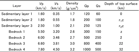
The velocity structure of the Osaka basin has been exten-sively investigated in recent years. Our initial model for the refinement was as follows. We adopted the 3D sediment-bedrock interface estimated by Afnimaret al.(2002), who carried out a joint inversion of refraction and gravity data. For the velocity structure of the bedrock, we used the same 1D stratified velocity structure model as in Yoshidaet al.
(1996). Table 1 lists this bedrock part and three sedimen-tary layers of the basin part of our initial model. The top surface of each sedimentary layer is set to be proportional to the depth of the sediment-bedrock interface. The common proportionality constants were estimated from microtremor array measurements and seismic reflection survey data by Kagawaet al.(2004).
The sediment-bedrock interfacezin Table 1 varies from station to station, and the depths of the top surfaces for sedimentary layers 2 and 3 arer1z andr2z, respectively,
wherer1andr2 are common proportionality constants. In
our refinement procedure, r1, r2, and zj (j = 1,2, . . .),
where j represents the number of stations, are treated as unknowns. We calibrated these unknowns using ground motion data from aftershocks.
We chose the three aftershocks listed in Table 2 as target events. Data from the Kobe area were used in the refinement because the velocity structure model in this area strongly affects 3D Green’s functions. They were recorded by the Committee of Earthquake Observation and Research in the Kansai Area (CEORKA), Iwataet al.(1996), and the Earth-quake Research Institute, University of Tokyo (see Nagano
et al., 1999).
In modeling ground motions, we calculated synthetic ve-locity waveforms using the finite element method (FEM) with voxel meshes (Koketsuet al., 2004; Ikegami et al., 2008) with intervals of 40 m. The source time function was a smoothed ramp function with a rise time of 0.5 s. Next, we checked whether the synthetic waveforms agreed with the observed ground motions in the frequency range 0.3–1.0 Hz. If not, we calibrated the depth z beneath a station and the common proportionality constantsr1andr2
by trial and error, then three-dimensionally combined them with the depths surrounding the station using the interpo-lating method of Smith and Wessel (1990). Thereafter, we again performed waveform modeling. We repeated this suc-cessive procedure until the synthetic waveforms fit the ob-served waveforms well with regard to their specific phases and travel times and the sum of squares of the residual of their waveforms shows the smallest value. In our refined model, the common proportionality constants r1 and r2,
which were 0.19 and 0.47 (Kagawaet al., 2004) in the ini-tial model, were revised to 0.08 and 0.39, respectively.
Figure 1 shows the resultant S-wave velocity structures beneath the stations and waveform comparisons for the af-tershock at 16:19 on February 2, 1995. The observed wave-forms were compared with the synthetic wavewave-forms com-puted with the initial and refined models.
3.
Source Inversion
Fig. 1. TheS-wave velocity structure beneath each station in the initial model (blue lines) and refined model (red lines), and comparison of transverse components for the aftershock at 16:19 on February 2, 1995, with the observed velocity waveforms (black traces), the synthetic waveforms calculated from the initial model (blue traces), and the refined model (red traces). The stations (red triangles) and three aftershocks (yellow stars) used in the refinement are plotted in the uppermost and leftmost map. The number above the traces is the maximum amplitude of the observed velocity waveform in cm s−1. TheS-wave velocity structure and waveforms at station KBU are not shown because the initial model of KBU is good enough
and therefore was not refined.
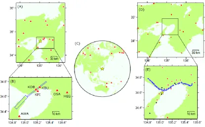
Fig. 2. Stations with (A) strong motions, (B) strong motions where 3D Green’s functions were calculated, (C) teleseismic body waves, and static displacements where (D) half-space and (E) 3D Green’s functions were calculated. The epicenter is marked by a yellow star. Red triangles in (A), (B) and (C) represent the stations. In (D) and (E), the stations that measure horizontal displacements (red), vertical displacements along a leveling route (blue) and three component displacements (black) are plotted. (B) also shows the two fault planes (blue rectangles).
as shown in Fig. 2. One fault plane is in Awaji Island and the other is in the Kobe area. The strike and dip of the for-mer were set as 43◦and 75◦, and those of the latter as 52◦ and 95◦. The two fault planes were divided into 4×4 km2
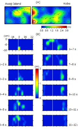
Fig. 4. (A) Final slip distribution obtained by the inversion, and (B) the growth of rupture depicted by the snapshots of slip distribution at every 1 s. Arrows and a white star in (A) denote subfault slips on the hanging walls and the hypocenter, respectively.
We introduced a positivity constraint to confine the slip an-gles within 180◦±45◦.
The fault model described above is the same as that of Yoshidaet al. (1996). However, they used only 1D
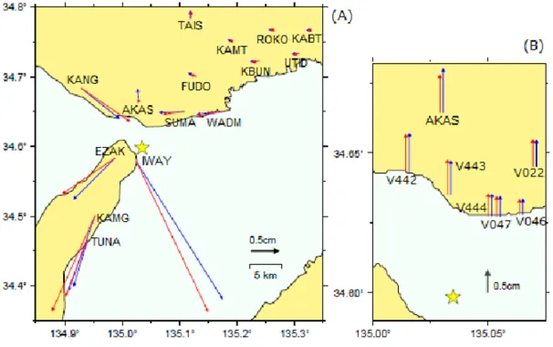
Fig. 5. Comparisons of the 3D (red arrows) and half-space (blue arrows) geodetic Green’s functions. (A) The horizontal displacements of the rake angle of 135◦for a subfault in the shallow part along the Nojima fault, and (B) the vertical displacements of the rake angle of 225◦for a subfault beneath the Akashi Strait, are shown. The yellow star represents the epicenter.
Fig. 6. Comparisons of the observed (black) and synthetic waveforms from inversion using 1D (blue) or 3D (red) Green’s functions at stations KOB, KPI and OSA. The maximum amplitude is given in cm s−1above each trace. Because the sensor orientation of the borehole seismometer at station
KPI has been corrected, the maximum amplitudes for the EW and NS components are different between the blue and red traces.
structure model refined as mentioned in the previous sec-tion for the strong-mosec-tion and geodetic data for the Osaka basin. We used the same Green’s functions as Yoshidaet al.
(1996) for the data outside the Osaka basin. The datasets shown in Fig. 2 and their time duration, weights, filtering and sampling were also the same as those in Yoshidaet al.
(1996). We note that the sensor orientation of the borehole seismometer installed at the strong-motion station KPI has been corrected.
For calculating 3D Green’s functions, we again used the FEM with voxel meshes. We then derived geodetic Green’s functions by averaging calculated ground motions from about 50 s to 70 s.
4.
Conclusions and Discussion
In this section, we summarize and discuss our results mainly by comparing them with those of Yoshida et al.
(1996).
In our source model, the rupture velocity for the first time window was set as 3.1 km/s, which is roughly equivalent to 90% of theS-wave velocity at the depth of the hypocenter
and provides the best fit to the observed data. This rupture velocity is higher than that of Yoshidaet al.(1996), which was 2.5 km/s. Unlike in the case of their model, the sed-imentary layers are included in our 3D velocity structure model. Since these additional sedimentary layers delay the travel times of 3D strong-motion Green’s functions at sta-tions inside the 3D basin structure, such as KOB and OSA (see Fig. 3(A)), the rupture velocity was set to be higher than that of Yoshidaet al.(1996) to compensate for these delays in the travel times. The rupture velocity in our model is also comparable with that of Horikawaet al.(1996), or Sekiguchi et al.(2000), both of whose velocity structure models include sedimentary layers.
Figure 4 illustrates the slip distribution and the snapshots of rupture during each of the 1-s time windows. The total seismic moment was estimated to be about 2.1×10¹⁹ N
m(Mw =6.8), which is slightly smaller than those of the
tions indicate uplift (see Fig. 5(B)), occurred to explain the considerable uplifts observed at the stations near the Akashi Strait. In addition, the larger-slip zone under the city center of Kobe spreads through a wider area than Wald (1996) and Yoshidaet al.(1996) indicated, and this zone probably con-tributed to the violent ground motions and extreme disaster in the city.
Figure 4(B) shows two rupture propagations in our source model. One propagated toward the shallow part along the Nojima fault, and the other propagated from the deeper part beneath the Akashi Strait to the zone beneath the city center of Kobe. This figure also shows a large slip around the hypocenter in the early stage, and this conse-quently contributes to the large final slip in this area.
The use of 3D strong-motion Green’s functions in our inversion resulted in a better fit to the observed strong mo-tions. For the strong motions, the variance reduction, which measures the degree of agreement between the observed and synthetic data, was nearly 10% higher than that in Yoshida et al. (1996). Figure 6 shows that the synthetic waveforms are generally consistent with the observations at the stations KOB, KPI and OSA in the Osaka basin. For the static displacements, we have confirmed that the de-gree of fit to the observed data was almost equivalent to that of Yoshidaet al.(1996). This indicates that static dis-placements are less sensitive to a 3D velocity structure than strong motions. Figure 5 shows the comparison of 3D and half-space geodetic Green’s functions, where only small differences can be seen.
Acknowledgments. We thank CEORKA, GSI, JMA, JUNCO,
the Kobe city government, Prof. Iwata (Kyoto Univ.), and Prof. Nagano (Tokyo Science Univ.) for providing data. We used GMT for drawing the figures. We also thank two reviewers Atsushi Nozu and Haruko Sekiguchi, and the Editor Tatsuhiko Hara for helpful comments.
References
Afnimar, K. Koketsu, and K. Nakagawa, Joint inversion of refraction and gravity data for the three-dimensional topography of a
sediment-lations of long-period ground motions: Japanese subduction-zone earth-quakes and the 1906 San Francisco Earthquake,J. Seismol.,12, 161– 172, 2008.
Iwata, T., K. Hatayama, H. Kawase, and K. Irikura, Site amplification of ground motions during aftershocks of the 1995 Hyogo-ken Nanbu Earthquake in severely damaged zone—array observation of ground motions at Higashinada ward, Kobe city, Japan,J. Phys. Earth,44, 553– 561, 1996.
Kagawa, T., B. Zhao, K. Miyakoshi, and K. Irikura, Modeling of 3D basin structures for seismic wave simulations based on available information on the target area: Case study of the Osaka Basin, Japan,Bull. Seismol. Soc. Am.,94, 1353–1368, 2004.
Katao, H., N. Maeda, Y. Hiramatsu, Y. Iio, and S. Nakao, Detailed mapping of focal mechanisms in/around the 1995 Hyogo-ken Nanbu Earthquake rupture zone,J. Phys. Earth,45, 105–119, 1997.
Kawase, H., The cause of the damage belt in Kobe: “The basin-edge effect,” Constructive interference of the direct S-wave with the basin-induced diffracted/Rayleigh waves,Seismol. Res. Lett.,67, 25–34, 1996. Kikuchi, M. and H. Kanamori, Rupture process of the Kobe, Japan, Earth-quake of Jan. 17, 1995, determined from teleseismic body waves, J. Phys. Earth,44, 429–436, 1996.
Koketsu, K., H. Fujiwara, and Y. Ikegami, Finite-element simulation of seismic ground motion with a voxel mesh,Pure Appl. Geophys.,161, 2183–2198, 2004.
Nagano, M., K. Kudo, and M. Takemura, Simulation analyses of the ar-ray strong motion records from the aftershocks of the 1995 Hyogo-ken Nanbu Earthquake (Mj =7.2) regarding the irregularity of the under-ground structure in Nagata ward, Kobe,J. Seismol. Soc. Jpn.,52, 25–41, 1999.
Sekiguchi, H., K. Irikura, and T. Iwata, Fault geometry at the rupture termination of the 1995 Hyogo-ken Nanbu Earthquake,Bull. Seismol. Soc. Am.,90, 117–133, 2000.
Smith, W. H. F. and P. Wessel, Gridding with continuous curvature splines in tension,Geophysics,55, 293–305, 1990.
Wald, D. J., Slip history of the 1995 Kobe, Japan, Earthquake determined from strong motion, teleseismic, and geodetic data,J. Phys. Earth,44, 489–503, 1996.
Wald, D. J. and R. W. Graves, Resolution analysis of finite fault source inversion using one-and three-dimensional Green’s functions, 2. Com-bining seismic and geodetic data,J. Geophys. Res.,106, 8767–8788, 2001.
Yoshida, S., K. Koketsu, B. Shibazaki, T. Sagiya, T. Kato, and Y. Yoshida, Joint inversion of near- and far-field waveforms and geodetic data for the rupture process of the 1995 Kobe Earthquake,J. Phys. Earth,44, 437–454, 1996.