F U L L P A P E R
Open Access
Idealized numerical experiments on microscale
eddies in the Venusian cloud layer
Masaru Yamamoto
Abstract
Three-dimensional microscale dynamics of convective adjustment and mixing in and around the Venusian lower cloud layer were investigated using an idealized Weather Research and Forecasting (WRF) model. As control parameters of the idealized experiment, the present work introduces an initial lapse rate in the convective layer and thermal flux associated with the infrared flux gap at cloud base. Eddy heat, material, and momentum fluxes
increase in the convective layer with the increase of these two parameters. In the case of convective adjustment over a very short period, prior to formation of a large-scale convective cell, transient microscale eddies efficiently and rapidly eliminate the convective instability. In the case of convective mixing induced by cloud-based thermal flux, mi-croscale eddies are induced around a thin unstable layer at the cloud base, and spread to the middle and upper parts of the neutral layer. For atmospheric static stability around 55 km, two types of fine structure are found: a wave-like pro-file induced by weak microscale eddies, and a propro-file locally enhanced by strong eddies.
Keywords:Venus; Atmospheric dynamics; Convection; Static stability
Background
On Venus, neutral and unstable layers were observed at height ranges of 50 to 55 km and less than 30 km (Seiff et al. 1980). The Vega 2 mission also observed zero and negative static stability in the lower clouds and near the surface (Young et al. 1987). The Venus Express radio science experiment (Tellmann et al. 2009) showed that the neutral and unstable layers around 50-km height extended to 45 km at high latitudes. Convective and tur-bulent motions have been observed in the Venusian neu-tral and unstable layers. The Vega balloon floated near 54 km (Sagdeev et al. 1986a), detecting vertical wind speeds of less than 1 m · s−1 during a quiet period, and greater than 3 m · s−1 during an active one (Sagdeev et al. 1986b). The observed convective heat flux ranged from 0 to 360 W · m–2(Ingersoll et al. 1987; Crisp et al. 1990).
Micro- and mesoscale atmospheric dynamics, which are divided by a spatial scale of around 2 km in the case of the Earth (Orlanski 1975), are important topics in me-teorology. Many works have conducted mesoscale simu-lations of the Venusian atmosphere. Baker et al. (1998,
2000a,b) simulated mesoscale convection and downward penetration with horizontal scales of 10 km around the 45-km level. However, microscale dynamics of turbulent convection on Venus have yet to be examined fully using a three-dimensional (3D) compressible and nonhydro-static model.
The Weather Research and Forecast (WRF) model (Skamarock and Klemp 2008) has been used extensively to forecast weather and regional climate on Earth, and has also been applied to other planets (Lee et al. 2006; Richardson et al. 2007; Newman et al. 2011). Moeng et al. (2007) applied WRF to large-eddy simulations of the Earth's planetary boundary layer. Recently, Yamamoto (2011) applied WRF to 3D idealized microscale simula-tions of the Venusian atmosphere, examining transport processes of convective adjustment and mixing near the surface. The present work focuses on small eddies with scales of a few kilometers and durations of hours in the neutral and unstable layers of Venusian clouds (50 to 55 km), excluding meso- and global-scale convection in a small model domain. The goals are to clarify transport processes of microscale convective adjustment and mixing in the lower cloud layer, and to compare the microscale features with lander and balloon observations. Model assumptions and a description are given in section Correspondence:[email protected]
Research Institute for Applied Mechanics, Kyushu University, 6-1 Kasuga-kouen, Kasuga 816-8580, Japan
‘Methods’. Results are discussed in section ‘Results and discussion’and summarized in section‘Conclusions’.
Methods
Model assumptions
The atmospheric rotation period (6 to 8 days), radiative timescale (1 to 10 days; Crisp and Titov 1997; Titov et al. 2013), and Venusian solar day (117 days) are lon-ger than that of the microscale eddy timescale (a few hours). Atmospheric radiative and rotational processes are not included, because the heating rate of approxi-mately 1 K · day−1(approximately 0.04 K h−1) and the ro-tation rate are not significant for dynamical phenomena with timescales of a few hours. In the present idealized simulation, the initial lapse rate of potential temperature ΓLAP and the turbulent thermal flux QB are set as tun-able parameters controlling microscale dynamics in the neutral layer.
PositiveΓLAP corresponds to the initial super adiabatic intensity leading to convective adjustment. The present work investigates turbulent eddies with temporal and spatial scales of a few hours and kilometers, resulting from convective adjustment (case A) under the initial unstable condition of positiveΓLAPin the Venusian lower cloud.
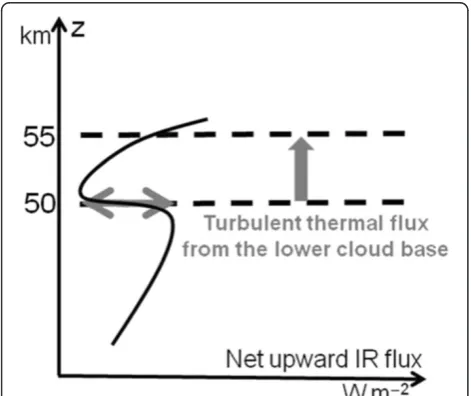
According to Lee and Richardson (2011), as vertical resolution was increased in their radiative-convective model, the gradient of net upward infrared (IR) flux in-creased at the cloud base (dashed line in Figure 1). This implies that the IR-flux gap (thick gray arrow in the figure) is located at the cloud base and that heating has a locally sharp peak (ideally a delta function). If the IR-flux has a broad gradient, the heating rate is trivial for timescales of a few hours. In contrast, if the heating
from the IR-flux gap is a delta function at cloud base, the local heating rate is very large. Such localized heating there (where the local IR flux changes discontinuously) is not resolved by the present model. Instead of using the delta function, therefore, it is parameterized as the turbulent thermal flux at the bottom of the neutral layer. This flux may result from subgrid-scale eddies,viarapid changes of cloud morphology and heating with finer-scale condensation/evaporation. Although it is difficult to observe and estimate the turbulent flux at the bound-ary of the convective condensation and stable evapor-ation regions, this does not necessarily mean that subgrid-scale thermal flux QB, associated with a dis-turbed cloud base and IR gap, can be neglected.
The turbulent thermal flux QBin the vertical integra-tion of the heat budget equaintegra-tion in the neutral layer is
QB≡θ′w′Bottom≈ 1 where [u]∇[θ] is heat advection, [QRAD] is radiative heat-ing, and ∂∂½ θt is the temperature tendency. Here, the square brackets indicate the area and time average over the model domain, and subscripts‘Bottom’and‘Top’ in-dicate the bottom and top of the neutral layer, respect-ively. Equation1is derived by vertical integration of
ρ ∂∂½ θ
The vertical integration of Equation2becomes
Z Top comes the vertically integrated budget equation (1).
The dynamical effect of long-lasting, large-scale mo-tions is introduced as the advection term of large-scale motions in Equation 1. In the present study,‘large scale’ means a horizontal size greater than that of the model domain (5 km). For an average over the large domain and a long period (square brackets in Equations 1 to 3), radiative heating should roughly balance the heat advec-tion of large-scale moadvec-tions. However, if there is transient subgrid-scale turbulence and an IR flux gap at the cloud base, [θ′w′]Bottom might be locally and transiently non-zero for a small domain. Thus, QB resulting from the subgrid-scale turbulence and IR flux gap should be con-sidered as a thermal forcing parameter at cloud base in microscale simulations with a small domain. Given the assumptions that (1) [QRAD] (approximately 0.04 K · h−1) induces large-scale circulation and convection [u] and
roughly balances their large-scale heat advection, (2) [θ′ w′]Topis nearly zero at the neutral layer top, and (3) [θ′ w′]Bottom is induced by transient subgrid-scale turbu-lence and the IR flux gap,QBis set as a tunable param-eter in accord with the radiative simulation and balloon experiment results. The present work investigates turbu-lent microscale eddies associated withQB(case B).
Model description
Fully compressible and nonhydrostatic idealized simula-tions were conducted using the WRF Advanced Re-search model (WRF-ARW ver. 3.2), with the Arakawa C-grid for grid staggering in the Cartesian coordinate system. We set the 3D model domain of area 5 × 5 km with 50 × 50 grid points, and a height range of 50 to 58 km with 80 levels. Reference pressure and temperature at the 50-km level are 1,000 hPa and 350 K, respectively.
The acceleration owing to gravity g is 8.87 m · s−2, the gas constant Ris 191.4 J · kg−1· K−1, the specific heat at constant pressure CP is 904.0 J · kg−1· K−1, and the mo-lecular weight of dry air is 44 g · mole−1. The rotational effect is not considered (the Coriolis parameter f is set to zero), because we focus on phenomena with time scales shorter than the atmospheric rotation. The third-order Runge-Kutta scheme is used for the time integra-tion. Rayleigh damping for vertical flow with an inverse time scale of 0.2 s−1 and depth of 1,000 m from the model top is preset.
To compute subgrid-scale eddy diffusion for turbulent mixing, 1.5-order turbulent kinetic energy (TKE) closure is used (Section 4.2.3 of Skamarock et al. 2008). The dif-fusion coefficient is obtained from an empirical constant CK, length scale l, and turbulent kinetic energye. CK is set to 0.1 (Xue et al. 2000), andl is defined by grid size, static stability, and turbulent kinetic energy. The subgrid-scale eddy diffusion could be sensitive to the empirical constants and grid scale, thereby influencing model results. At the present stage, it is difficult to apply higher resolution to the parameter sweep experiment under various initial and bottom-boundary conditions, because of the large computational resources required. Experiments investigating the sensitivity to grid size and subgrid-scale parameterization are necessary for future model validation.
The slip bottom boundary condition (i.e., drag coeffi-cient set to zero) is used in all simulations, so the bot-tom momentum flux is set to zero. Fluxes of a passive tracer and heat at the bottom boundary are taken as zero and parameter QB (K m · s−1), respectively. Thus, the surface layer scheme is not applied in the model.
Table 1 Model conditions
A double periodic boundary condition is used along x (along the latitude line) and y (along the longitude line).
ΓLAPis an initial lapse rate of potential temperature, and is defined as −dθ=dz in an initially neutral or unstable
layer (50 to 55 km), which is capped by a stable layer (55
to 58 km) with buoyancy frequencyN (≡gdlnθ=dz1=2) of 0.01 · s−1. In addition, a random perturbation is imposed on the mean temperature field at the lowest four grid levels, to initiate turbulent motion.
Figure 3Maximum area-mean magnitudes of (a)θ′w′ (K m · s–1), (b)q′w′ (m · s–1), and (c)u′w′ (m2· s–2).For cases A02 to A30, solid
circles, pluses, crosses, and triangles represent results forUZvalues of 0, 1, 2, and 3 m · s–1· km–1, respectively.
Figure 4Time-height cross sections of area-meanθ′w′(upper panels) andq′w′(lower panels).These fluxes normalized by maximum flux magnitudes in Figure 3 are calculated from the experiments under the conditionUZ= 0 m · s–1· km–1for(a)case A02,(b)case A10, and(c)case
A20. Thick contours in upper and lower panels show area-mean potential temperature (K) and mixing ratio (q× 106; kg · kg–1), respectively.
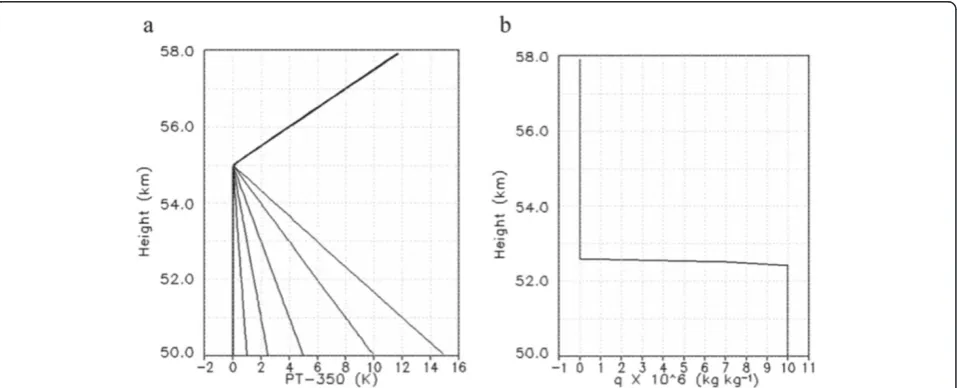
The experimental conditions ofΓLAPandQBare listed in Table 1. Initial profiles of potential temperatureθand passive tracer mixing ratio qare shown in Figure 2. The convective adjustments are simulated in case A (A02 to A30, section ‘Convective adjustment in unstable layer (case A)’). ΓLAP ranges from 0.2 to 3.0 K · km−1 in the neutral layer, andQBis set to zero. Microscale eddies in-duced byQBare simulated in case B (B1 to B5, section
‘Microscale eddies induced by turbulent thermal flux (case B)’).QBis varied from 0.001 to 0.256 K m · s−1. The wide range of QB, from 1.44 to 369 W · m–2 (ρ= 1.594 kg · m–3,Cp= 904 · kg−1· K−1at 50 km, Seiff et al. 1985), covers the convective heat flux observed in the Vega bal-loon experiments (0 to 360 W · m–2; Crisp et al. 1990; Ingersoll et al. 1987) and the IR-flux gap at cloud base (20 W · m–2; Lee and Richardson 2011). ΓLAP is set to 0 K · km−1.
The vertical shear of the initial horizontal wind UZis set to 0 m · s−1· km−1in cases A and B. In addition, sen-sitivity simulations for initial wind shears 1, 2, and 3 m · s−1· km−1 were also run to investigate the influence of the differentials between zonal winds in the lower and upper cloud layers. To confirm the presence of micro-scale eddies in the large model domain, domain size (5 × 5 km) in sections ‘Convective adjustment in un-stable layer (case A)’and ‘Microscale eddies induced by
turbulent thermal flux (case B)’ is extended by a factor of four (to 20 × 20 km) in the large-domain experiment (section ‘Sensitivity of microscale eddies to model do-main size’).
Results and discussion
Convective adjustment in unstable layer (case A)
The initial lapse rateΓLAP ¼−dθ=dz
is set as a control parameter of convective adjustment in case A.
Max-imum magnitudes of area-mean θ′w′,q′w′, andu′w′ in-crease withΓLAP, as shown in Figure 3. Here, the overbar and prime indicate the zonal average and deviation from average, respectively. Eddy heat, material, and momen-tum transport are more efficient for larger ΓLAP. The
maximumθ′w′andu′w′are sensitive to vertical shear of the initial zonal windUZfor largeΓLAP. In particular,u′w′ is amplified by increasingUZ, although there are a few ex-ceptions. For material transport, there are large differences
of maximumq′w′ among the fourUZcases for the entire range ofΓLAP.
Figure 4 shows time-height cross sections of
area-meanθ′w′andq′w′in cases A02 to A20. The initial con-vective adjustment causes upward eddy fluxes of heat
Figure 5Time-height cross sections of area-meanu′w′inUZ= 0 and 3 (m · s−1· km−1; upper and lower panels, respectively).These fluxes
and material. The convective adjustment occurs around 1 h in case A02, and 45 min in cases A10 and A20. With increasingΓLAP, eddy kinetic energy increases in the neu-tral or unstable layer, and static stability (dθ/dz) around 56 km weakens owing to penetration into the upper stable layer. Although the top of the mixed layer rises slightly with increasing ΓLAP, the convective adjustment does not significantly influence the upper stable layer throughout the simulation.
The eddy momentum flux is sensitive to the initial verti-cal shear of zonal flow UZ. Figure 5 shows time-height
cross sections of area-mean u′w′ for UZ values 0 and 3 m · s−1· km−1. Large fluxes are evident at the time of con-vective adjustment. Structures of the mean flow and eddy momentum transport are complicated in the case of an initially zero wind-shear state (UZ= 0 m · s−1· km−1), and velocities and fluxes fluctuate randomly with small ampli-tudes. In contrast, downward u′w′ is predominant in the presence of a large initial wind shear (UZ= 3 m · s−1· km−1). A narrow shear zone of the zonal flow develops around the mixed layer top (where contour intervals of mean zonal flow are dense), and weak shear persists in the upper part of the mixed layer after the convective adjustment.
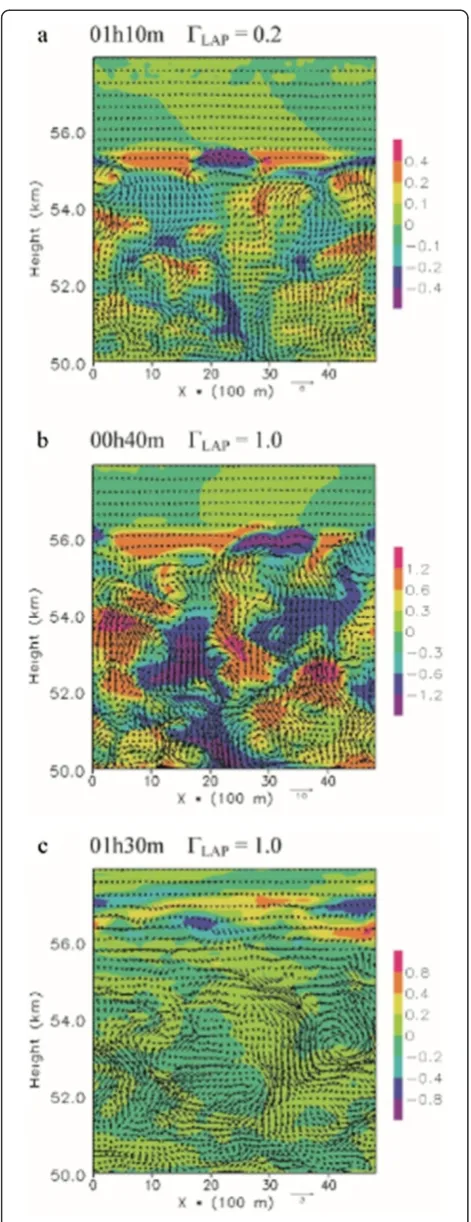
Figure 6 shows snapshots of eddy wind velocity and potential temperature for weak and strong convective adjustments. Transient eddies with scales of a few kilo-meters are predominant in the unstable layer, but they are not found in the upper stable layer. After the strong convective adjustment penetrates the stable layer (to ap-proximately 56 km), gravity waves are generated in its upper portion (Figure 6c), where the static stability has a wave-like profile (not shown).
Microscale eddies induced by turbulent thermal flux (case B)
QBis set as a control parameter of convective mixing in case B. Figure 7 shows maximum magnitudes of
area-meanθ′w′,q′w′, andu′w′. These flux magnitudes increase withQB. We see large differences ofθ′w′andu′w′among the fourUZcases. Initially, strong shear of the zonal flow
(UZ= 3 m · s–1· km–1) is likely to produce large θ′w′ (left
panel of Figure 7) andu′w′(right panel).
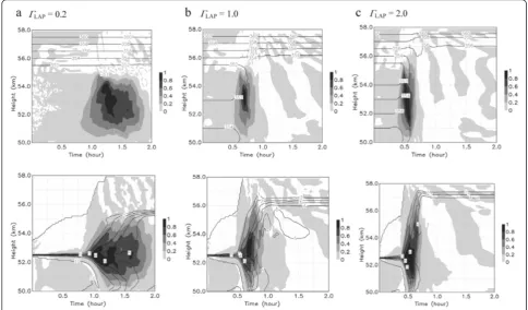
Time-height cross sections of area-meanθ′w′for cases B1, B3, and B5 are shown in the upper panels of Figure 8.
Figure 6Zonal-vertical distributions ofV′andθ′at locationy= 1,000 m.The eddy components of wind velocityV(m · s–1; arrows) and potential temperatureθ(K; shaded) are calculated from the experiments under the conditionUZ= 0 m · s–
1
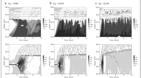
In the case of small QB(=0.001 K m · s–1), although the eddy upward heat flux is inefficient, weak mixing occurs throughout the simulation. For a QBof 0.016 K m · s–1, substantial upward heat transport is evident below 52 km and downward heat fluxes are apparent near 55 km
during the calculation. For large QB (=0.256 K m · s–1), the vertical scale of the neutral layer grows gradually with time. The upward fluxes decrease rapidly with height and strong fluxes are confined near 50 km. Large QB at the bottom (values ≥0.016 K m · s–1) heats the
Figure 7Maximum area-mean magnitudes of (a)θ′w′(K m · s–1), (b)q′w′ (m · s–1), and (c)u′w′(m2· s–2).For cases B1 to B5, solid circles, pluses, crosses, and triangle symbols represent results forUZvalues 0, 1, 2, and 3 m · s–1· km–1, respectively.
Figure 8Time-height cross sections of area-meanθ′w′(upper panels) andq′w′(lower panels).These fluxes normalized by maximum flux magnitudes in Figure 7 are calculated from the experiments under the conditionUZ= 0 m · s–1· km–1for(a)case B1,(b)case B3, and(c)case B5.
Thick contours in upper and lower panels show area-mean potential temperature (K) and mixing ratio (q× 106; kg · kg–1), respectively.
mixing layer via heat flux convergence of microscale eddies.
The passive tracer is transported rapidly upward with the initial convection (lower panels of Figure 8). After this, a uniform distribution forms in the neutral layer. A strong gradient of the tracer forms at the boundary be-tween the neutral and stable layers.
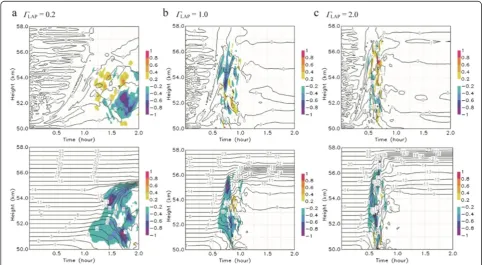
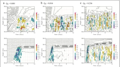
Figure 9 shows time-height cross sections of area-mean
u′w′ for UZ values of 0 and 3 m · s–1· km–1. The area-mean eddy momentum flux and zonal flow change ran-domly in the neutral layer in the initially zero wind-shear state (UZ= 0 m · s–1· km−1in the upper panels of Figure 9). In contrast, in cases of initially large shear (lower panels of
the figure), downward u′w′ is predominant upon the initial convection. Afterward, the shear zone of zonal flow develops at the boundary between the lower neutral and upper stable layers, and this zone persists because shear instability does not ensue. In contrast to small QBvalues (≤0.016 K m · s–1), random disturbances of area-mean eddy momentum flux and zonal flow occurs in the mixing layer following the initial strongest momentum mixing with largeQB(=0.256 K m · s–1in the lower right panel of Figure 9). Such strong wind shear forms via convective adjustment (Figure 5) and turbulent mixing (Figure 9).
Comparison with the balloon experiments is useful for discussing dynamical similarities with the observations and for qualitatively understanding the formation mech-anism of fine structures; however, it is difficult to make a quantitative comparison in the idealized model configur-ation. Figure 10 shows the time series of vertical wind and eddy heat flux. The Vega balloon floated near 54 km (Sagdeev et al. 1986a) and detected vertical wind speeds less than 1 m · s−1during a quiet period and greater than 3 m · s−1 during an active period (Sagdeev et al. 1986b). Downward winds were predominant as measured by the balloon, whereas there are both upward and downward motions in the model. This difference might be ex-plained by the absence of large-scale circulation and ra-diation in the model, or by the dependence of vertical motions on the sampling locations. Observed convective heat flux ranged from 0 to 100 W · m–2 and increased abruptly to 360 W · m–2(Ingersoll et al. 1987; Crisp et al. 1990). At 55 km (ρ= 0.9207 kg · m–3,Cp= 859 kg−1· K−1; Seiff et al. 1985), the observed heat flux 100 W · m–2 equals that forθ′w′= 0.126 K · m s–1. The eddy heat fluxes fluctuate slightly during the simulation, but large fluxes appear intermittently. The maxima of 30, 320, and 480 W · m–2, which are larger thanQB, occur in cases B3, B4, and B5, respectively. The abrupt increase of convective
Figure 10Time histories of vertical wind velocities (m · s−1; left panels) and eddy heat fluxes (K m · s−1; right panels).These are plots of
heat flux in case B4 is comparable to that observed in the Vega experiment (360 W · m–2). This indicates the possi-bility that intermittent microscale eddies generate such an increase.
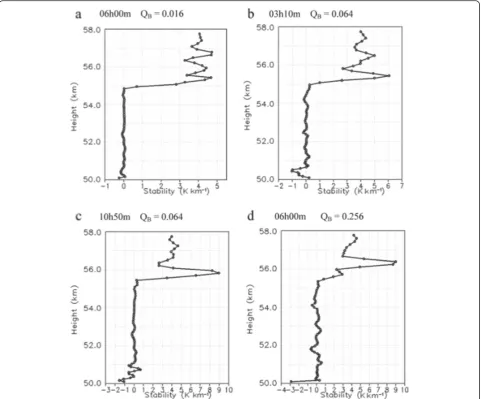
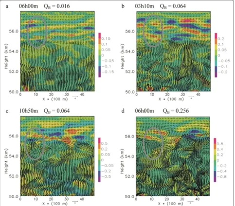
Figure 11 shows vertical profiles of the atmospheric static stability. Wave-like fluctuations are evident in the stable layer above 55 km in the upper panels of the figure. These correspond to a temperature pattern in-duced by gravity waves of short vertical wavelength of approximately 1 km and small amplitude of approxi-mately 0.1 K in the upper stable layer (gray ellipses in upper panels of Figure 12). These gravity waves are forced by turbulent microscale eddies and not by strong deep convective penetration of the upper stable layer. Such small-scale gravity waves were not generated by the large-scale convection cited in Baker et al. (1998).
However, local and frequent penetrations maintained by turbulent microscale eddies might force such gravity waves. In the lower panels of Figure 11, static stability increases locally to approximately 10 K · km−1around 56 km. This locally enhanced structure is caused by a temperature patch resulting from the strong turbulent ed-dies (gray ellipses in lower panels of Figure 12). Such local increase of stability is also seen above 55 km in the Pion-eer Venus and Vega observations (Young et al. 1987). The transient nature and local amplitude of microscale eddies around 55 km determines the static stability pattern. When the eddies strengthen (weaken) around the top of the neutral layer, the locally enhanced (wave-like) struc-ture is likely to appear in the upper stable layer.
In contrast to the upper stable layer, transient eddies of scales 1 to 2 km are predominant in the convective
layer. However, eddy temperatures in the neutral layer are smaller than those above 56 km (Figure 12). Thus, the small temperature deviation associated with micro-scale convective motions results in small fluctuations of static stability in the convective layer (50 to 55 km; Figure 11).
Sensitivity of microscale eddies to model domain size
Sensitivity to model domain size is investigated for sev-eral cases to confirm the presence of the microscale ed-dies in a large domain of 20 × 20 km. The domain area is 16 times larger than in sections ‘Convective adjust-ment in unstable layer (case A)’and ‘Microscale eddies
induced by turbulent thermal flux (case B)’. Figure 13
shows time-height cross sections of area-meanθ′w′,q′w′,
and u′w′ for large-domain experiments of cases A10 and B3 under the conditionUZ= 0 m · s–1· km–1. In the case of convective adjustment, time histories and magnitudes of eddy heat and material fluxes in the large domain ex-periment (case A10L) are nearly the same as those of case A10. The area-mean zonal wind becomes smooth in case A10L. The area-mean wind shear inducing the eddy mo-mentum flux also weakens because the zonal flow is aver-aged over the large domain. Thus, the area-mean maximum eddy momentum flux for case A10L is one-third less than that of case A10. In the case of convective
Figure 12Zonal-vertical distributions ofV′andθ′at locationy= 1,000 m.The eddy components of wind velocityV(m · s–1; arrows) and potential temperatureθ(K; shaded) are calculated from the experiments under the conditionUZ= 0 m · s–1· km–1at(a)360 min for case B3,(b)
mixing induced byQB, maximum eddy heat and material fluxes in case B3L are the same as those in B3 (differences were only a few percent). However, the large flux regions (red shading) are somewhat wider in the large-domain ex-periment (Figure 13d). The random fluctuation and verti-cal shear of the mean zonal wind becomes smooth, and the area-mean momentum flux associated with the mean wind shear also weakens in the large-domain experiment.
Figure 14a,b shows horizontal distributions at 54 km of eddy components of wind (m · s–1; arrows) and poten-tial temperature (K; shaded) for convective adjustment in case A10L, and strong convective mixing in case B3L. Turbulent eddies with sizes equal to and smaller than 5
km are predominant in the large-domain experiments. Strong microscale eddies are relatively dense in A10L. In contrast, microscale eddies are relatively sparse and weak in B3L. Figure 14c,d shows amplitudes of the Fourier component of potential temperature for each zonal wavelength, averaged over an extended sampling area of 25.6 × 25.6 km. Here, we assumed that the wave structures are cyclically repeated outside the model do-main. This was done to analyze the output data with a double periodic boundary under the same condition in which the sampling number was 28 and the data grid interval was 100 m in the fast Fourier transform. Signals with zonal wavelengths of 2.5 and 5 km are predominant (See figure on previous page.)
Figure 13Time-height cross sections of area-meanθ′w′(left panels),q′w′(middle panels), andu′w′(right panels).These fluxes (shaded) are calculated from the experiments under the conditionUZ= 0 m · s–1· km–1for(a)case A10,(b)case A10L,(c)case B3, and(d)case B3L. Thick
contours show area-mean potential temperature (K; left panels), mixing ratio (q× 106; kg · kg–1; middle panels), and wind speed (m · s–1; right panels).‘L’appended to the case name indicates large-domain experiment.
Figure 14Horizontal distributions (a,b; upper panels) and amplitudes of Fourier components (c,d; lower panels) of potential temperature.
These are plots of eddy components of wind (m · s–1; arrows) and potential temperature (K; shaded) at 54 km under the conditionUZ= 0 m · s–1· km–1
in these experiments. The strongest signals are enhanced by 50% in the small-domain experiments, because of wave structure repetition under the cyclic condition every 5 km. In contrast, strong small-scale eddies ran-domly (not cyclically) occur in the large domain. The strong but sparse small-scale eddies along the x direc-tion are partly decomposed to Fourier components of large scales >5 km. Thus, the strongest signals at 5 km become small in the large-domain experiments, relative to the small-domain experiments.
When a sub-domain of x= 0 to 5 km and y= 0 to 5 km is considered in the large-domain experiments, sig-nals of zonal wavelengths >5 km do not predominate in the sub-domain. Zonal-vertical cross sections of eddies in the sub-domain of 5-km size in the large-domain ex-periments (Figure 15) are similar to those of the small-domain experiments (Figure 12). Weak turbulent eddies in case B3L induce gravity waves in the upper stable layer, resulting in a wave-like profile of static stability above 55 km. Conversely, strong microscale eddies in case B4L produce temperature patches on scales of ap-proximately 2 km, which are locally enhanced around 55.5 km at x= 1,000 m. This produces a locally en-hanced profile of static stability. Thus, these results in the large-domain simulation are consistent with those in section ‘Microscale eddies induced by turbulent thermal flux (case B)’.
As mentioned above, 3D microscale eddies are pre-dominant in the large-domain simulations (20 × 20 km) as in the simulations with domains of 5 × 5 km. Model domain size does not greatly influence the turbulent mesoscale eddies and their heat and material transports, although the momentum flux magnitude decreases in the initially zero wind-shear experiments. In the pres-ence of turbulent microscale eddies, the following two processes are important: (i) In the case of convective
adjustment over very short periods (10 to 30 min), be-fore a large-scale convection cell forms, the transient turbulent eddies efficiently and rapidly eliminate the ini-tially unstable state. (ii) In the case of convective mixing induced by QB, because forcing ofQBis confined to the cloud base and is maintained, strong eddies of 1-km length are induced around a thin unstable layer at the cloud base (around 50 km in Figure 11) and spread to the middle and upper parts of the neutral layer. Thus, the microscale eddies are maintained, and eddy heat fluxes are large in the lower part of the neutral layer. Such microscale features in (i) and (ii) are not found in previous mesoscale simulations.
Conclusions
The present work investigated 3D microscale dynamics of convective adjustment and mixing in and around the Venusian lower cloud layer, and examined heat, material, and momentum transport processes of microscale eddies. In an idealized WRF model, initial lapse rate and bottom thermal flux are given as control parameters of microscale adjustment and mixing in the lower cloud layer between 50 and 55 km. Eddy heat, material, and momentum fluxes are enhanced in the lower cloud layer with increasing initial lapse rate in the unstable layer and bottom thermal flux in the neutral layer. When shear of the zonal wind is initially present, a strong thin shear zone of zonal wind is able to form around the top of the convective layer after the initial strong convective motions, and momentum flux magnitudes somewhat in-crease. The eddy heat and material fluxes are not sensi-tive to model domain size. However, because the random fluctuation and vertical shear of the mean zonal wind become smooth in the large-domain experiment, area-mean momentum flux associated with the shear weakens in the initially zero wind-shear experiments.
Thus, we should carefully ascertain the dependence of vertical eddy momentum transport on domain size.
If convective adjustment andQB-induced mixing occur in the Venusian lower cloud, microscale eddies should be considered in eddy heat and material transport pro-cesses. In the case of convective adjustment over very short periods (10 to 30 min), before a large-scale con-vection cell forms, the transient microscale eddies effi-ciently and rapidly eliminate the initially unstable state. In the case of convective mixing induced byQB, because forcing ofQBis confined to the cloud base and is main-tained, strong small eddies are initially induced around a thin unstable layer at the cloud base and spread to the middle and upper parts of the neutral layer.
Weak turbulent eddies induce microscale temperature patches associated with gravity waves in the upper stable layer, and thereby form a wave-like profile of static sta-bility above 55 km. Such small turbulent eddies may contribute to the forcing mechanism of gravity waves. Conversely, strong microscale eddies produce locally en-hanced structures of atmospheric stability. Since ampli-tudes of the microscale turbulent eddies are large around the mixing layer top, the locally enhanced struc-tures are likely to appear in the upper stable layer.
Competing interests
The author declares that he has no competing interests.
Acknowledgements
This work was supported by the Japan Society for the Promotion of Science (JSPS) and Ministry of Education, Culture, Sports, Science and Technology of Japan (MEXT) Grants-in-Aid for Scientific Research (KAKENHI grant numbers 22244060 and 23540514), and the cooperative research project of the Atmosphere and Ocean Research Institute, The University of Tokyo. Numerical experiments were conducted at the Information Technology Center of The University of Tokyo and the Research Institute for Information Technology of Kyushu University.
Received: 27 June 2012 Accepted: 21 November 2013 Published: 30 April 2014
References
Baker RD, Schubert G, Jones PW (1998) Cloud-level penetrative compressible convection in the Venus atmosphere. J Atmos Sci 55:3–18
Baker RD, Schubert G, Jones PW (2000a) Convectively generated internal gravity waves in the lower atmosphere of Venus: part I: no wind shear. J Atmos Sci 57:184–199
Baker RD, Schubert G, Jones PW (2000b) Convectively generated internal gravity waves in the lower atmosphere of Venus: part II: mean wind shear and wave–mean flow interaction. J Atmos Sci 57:200–215
Crisp D, Titov DV (1997) The thermal balance of the Venus atmosphere. In: Bougher SW, Hunten DM, Phillips RJ (ed) Venus-II. The University of Arizona Press, Tucson, Arizona
Crisp D, Ingersoll AP, Hildebrand CE, Preston RA (1990) VEGA balloon meteorological measurements. Adv Space Res 10:109–124
Ingersoll AP, Crisp D, Grossman AW (1987) Estimates of convective heat fluxes and gravity wave amplitudes in the Venus middle cloud layer from VEGA balloon measurements. Adv Space Res 7:343–349
Lee C, Richardson MI (2011) A discrete ordinate, multiple scattering, radiative transfer model of the Venus atmosphere from 0.1 to 260μm. J Atmos Sci 68:1323–1339
Lee C, Richardson MI, Newman C, Toigo AD (2006) Venus WRF: a new Venus GCM using Planet WRF. Bull Am Astron Soc 38:526
Moeng C-H, Dudhia J, Klemp J, Sullivan P (2007) Examining two-way grid nesting for large eddy simulation of the PBL using the WRF model. Mon Weather Rev 135:2295–2311
Newman CE, Lee C, Lian Y, Richardson MI, Toigo AD (2011) Stratospheric superrotation in the Titan WRF model. Icarus 213:636–654
Orlanski I (1975) A rational subdivision of scales for atmospheric processes. Bull Am Meteorol Soc 56:527–530
Richardson MI, Toigo AD, Newman CE (2007) Planet WRF: a general purpose, local to global numerical model for planetary atmospheric and climate dynamics. J Geophys Res 112:E09001. doi:10.1029/2006 JE002825 Sagdeev RZ, Linkin VM, Blamont JE, Preston RA (1986a) The Vega Venus balloon
experiment. Science 231:1407–1408
Sagdeev RZ, Linkin VM, Kerzhanovich VV, Lipatov AN, Shurupov AA, Blamont JE, Crisp D, Ingersoll AP, Elson LS, Preston RA, Hildebrand CE, Ragent B, Seiff A, Young RE, Petit G, Boloh L, Alexandrov YN, Armand NA, Bakitko RV, Selivanov AS (1986b) Overview of VEGA Venus balloon in situ meteorological measurements. Science 231:1411–1414
Seiff A, Kirk DB, Young RE, Blanchard RC, Findlay JT, Kelly GM, Sommer SC (1980) Measurements of thermal structure and thermal contrasts in the atmosphere of Venus and related dynamical observations: results from the four Pioneer Venus probes. J Geophys Res 85:7903–7933
Seiff A, Schofield JT, Kliore AJ, Taylor FW, Limaye SS, Revercomb HE, Sromovsky LA, Kerzhanovich VV, Moroz VI, Marov MY (1985) Models of the structure of the atmosphere of Venus from the surface to 100 kilometers altitude. Adv Space Res 5:3–58
Skamarock WC, Klemp JB (2008) A time-split nonhydrostatic atmospheric model for weather research and forecasting applications. J Comput Phys 227:3465–3485 Skamarock WC, Klemp JB, Dudhia J, Gill DO, Barker DM, Duda MG, Huang X-Y,
Wang W, Powers JG (2008) A description of the advanced research WRF version 3. NCAR/TN-475 + STR, NCAR, Boulder, Colorado
Tellmann S, Pätzold M, Häusler B, Bird MK, Tyler GL (2009) Structure of the Venus neutral atmosphere as observed by the Radio Science experiment VeRa on Venus Express. J Geophys Res 114:E00B36. doi:10.1029/2008 JE003204 Titov DV, Piccioni G, Drossart P, Markiewicz WJ (2013) Radiative energy balance in
the Venus atmosphere. In: Bengtsson L, Bonnet R-M, Koumoutsaris GD, Lebonnois S, Titov D (ed) Towards understanding the climate of Venus, ISSI scientific report series, vol 11. Springer, New York, pp 23–53
Xue M, Droegemeier KK, Wong V (2000) The advanced regional prediction system (ARPS) - a multi-scale nonhydrostatic atmospheric simulation and prediction model: part I: model dynamics and verification. Meteorol Atmos Phys 75:161–193
Yamamoto M (2011) Microscale simulations of Venus' convective adjustment and mixing near the surface: thermal and material transport. Icarus 211:993–1006 Young RE, Walterscheid RL, Schubert G, Seiff A, Linkin VM, Lipatov AN (1987)
Characteristics of gravity waves generated by surface topography on Venus: comparison with the VEGA balloon results. J Atmos Sci 44:2628–2639
doi:10.1186/1880-5981-66-27
Cite this article as:Yamamoto:Idealized numerical experiments on microscale eddies in the Venusian cloud layer.Earth, Planets and Space
201466:27.
Submit your manuscript to a
journal and benefi t from:
7 Convenient online submission
7 Rigorous peer review
7 Immediate publication on acceptance
7 Open access: articles freely available online
7 High visibility within the fi eld
7 Retaining the copyright to your article