R E S E A R C H
Open Access
Cognitive radar ambiguity function
optimization for unimodular sequence
Jindong Zhang, Xiaoyan Qiu
*, Changli Shi and Yue Wu
Abstract
An important characteristic of a cognitive radar is the capability to adjust its transmitted waveform to adapt to the radar environment. The adaptation of the transmit waveform requires an effective framework to synthesize
waveforms sharing a desired ambiguity function (AF). With the volume-invariant property of AF, the integrated sidelobe level (ISL) can only be minimized in a certain area on the time delay and Doppler frequency shift plane. In this paper, we propose a new algorithm for unimodular sequence to minimize the ISL of an AF in a certain area based on the phase-only conjugate gradient and phase-only Newton’s method. For improving detection performance of a moving target detecting (MTD) radar system, slow-time ambiguity function (STAF) is defined, and the proposed algorithm is presented to optimize the range-Doppler response. We also devise a cognitive approach for a MTD radar by adaptively altering its sidelobe distribution of STAF. At the simulation stage, the performance of the proposed algorithm is assessed to show their capability to properly shape the AF and STAF of the transmitted waveform. Keywords: Cognitive radar, Unimodular sequence synthesis, Optimization algorithm, Ambiguity function, Slow-time ambiguity function
1 Introduction
Cognitive radar (CR) is established by the notion of a cog-nitive cycle, in which the two key aspects are perception of the environment and control exercised on the envi-ronment by virtue of feedback of the information that was learnt through perception. Figure 1 summarizes the essence of cognitive radar in its most basic forms. In cog-nitive radar system, how the transmitted waveform adapts in response to information about the radar environment is a key enabling step [1]. Many of the research efforts have been devoted to radar waveform optimization methods, which have been developed based on different perfor-mance objectives. For detecting a particular target in the presence of additive signal-dependent noise, waveform optimization method, developed by Guerci [2, 3], is evalu-ated in terms of the signal-to-interference-plus-noise ratio (SINR) under a particular model of the system, interfer-ence, clutter, and targets. For estimating the parameters of a target from a given ensemble, the radar waveform should be designed to maximize the mutual information
*Correspondence: [email protected]
College of Electronic and Information Engineering, Nanjing University of Aeronautics and Astronautics, Nanjing 210016, China
(MI) between the received signal and the target ensem-ble [4]. Besides, exploiting a variety of knowledge sources, the radar can locate the range-Doppler bins where strong unwanted returns are predicted and synthesize a wave-form whose ambiguity function (AF) exhibits low values in those interfering bins. In the previous work in [5], the idea of designing the slow-time ambiguity function (STAF) of the transmit waveform in a CR system has been discussed.
In radar systems, unimodular (i.e., constant modulus) sequences are usually exploited and optimized for trans-mission. The integrated sidelobe level (ISL) of the autocor-relation function (ACF) is often used to express the good-ness of the correlation properties of a given sequence. A transmitted sequence with low ISL value reduces the risk that the echo signal of the weak target of interest is drawn in the sidelobes of the strong one or clutter interference [6]. Additionally, the unimodular sequence has low peak-to-average power ratio (PAR) which is especially desired for the transmitter [7]. A lot of literature has been focused on the topic of unimodular sequence synthesis with good properties (in particular, the ACF with low ISL values) and the many references included. These unimodular synthe-sis methods can be summarized into two types. The first
Fig. 1Cognitive radar in its most basic form
is to use some famous sequences, such as the Golomb sequence [8], Frank sequence [9], and a pseudo random sequence, which have been proved with low sidelobes and applied in the radar systems successfully. The second is to synthesize the sequence with minimized ISL metric by the optimization algorithms [10–12]. Because the problem of reducing the ISL metric may have multiple local min-ima, the exhaustive search algorithm has been proposed in [12]. The computational burden of this kind of algorithm increases significantly as the sequence length increases. Some optimization algorithms have been designed as the local minimization algorithms to overcome this default [13–17]. Most of these algorithms can obtain fast conver-gence in descent gradient and provide quick solutions. It is worthwhile to mention that the cyclic algorithms pro-posed in [13] can design unimodular sequences that have virtually zero autocorrelation sidelobes in a specified lag interval and long sequences.
In this paper, we mainly consider the ambiguity function synthesis problem for unimodular sequences. According to Woodward’s definition, AF is a two-dimensional func-tion defined on the time delay and Doppler frequency shift plane. The AF is defined as follows:
χ(τ,fd)= ∞
−∞s(t)s
∗(t+τ)ej2πfdtdt, (1)
where τ andfd denote the time delay and Doppler fre-quency shift, respectively, ands(t)is the radar waveform. It describes the matched filter response to the target sig-nature. The shape of AF indicates the range and Doppler resolutions of the radar system. It also demonstrates the matched filter output with respect to the interference pro-duced by unwanted returns. It should come with no sur-prise that extensive research on AF synthesis exists in the literature [18–23]. Despite so much effort on this problem, few methods can synthesize the desired AF successfully. In [22], the cross ambiguity function was considered instead of AF. A pair of the waveform and receiving filter was developed simultaneously. Aubry et al. [23] deal with the design of phase-coded pulse train, which approximately maximizes the detection performance. A similarity con-straint between the ambiguity functions of the devised waveform and the pulse train encoded with the prefixed sequence is required. De Maio et al. [5] also discuss the design problem of phase-coded pulse train. The average
value of the STAF of the transmitted signal over some range-Doppler bins is minimized with prior information.
Note that the volume of a AF, which is defined as
V=
∞
−∞ ∞
−∞|χ(τ,fd)|
2dτdf
d (2)
is equal to the energy ofs(t). The volume-invariant prop-erty of AF prevents the synthesis of an ideal AF that has a high narrow peak in the origin and zero sidelobes every-where else. In this paper, we mainly focus on the synthesis of an AF that has a clear area close to the origin or mini-mized ISL in a certain area on the time delay and Doppler frequency shift plane.
Additionally, it is known that a moving target detect-ing (MTD) radar system is designed to observe the target in range-Doppler bins [6]. Its detection performance is considerably affected by the range-Doppler response of the waveform used to illuminate the operation environ-ment. Considering that a MTD radar transmits a burst of pulses in slow time, the STAF is defined to evaluate the range-Doppler response.
The main contribution of this paper is as follows:
(1) For optimizing the shape of an AF, the optimization algorithm is proposed based on the phase-only conjugate gradient (POCG) and phase-only Newton’s method (PONM), which have been successfully applied in optimizing the phased array radar beam pattern.
(2) We extend the PCA and present an algorithm for optimizing the shape of STAF.
(3) A cognitive approach for a MTD radar system is also provided in this work. The radar system can adaptively alternate its sidelobe distribution of STAF according to the interested area and clutter
distribution on the time delay and Doppler frequency shift plane. This scheme is especially attractive for detecting a target with a small radar cross section (RCS) in a heavy clutter scenario.
radar system. A cognitive workflow is also given. Several numerical examples are presented in Section 4. Finally, concluding remarks and directions for future research are presented in Section 5.
2 Ambiguity function synthesis
2.1 Problem formulation
We consider a monostatic radar that transmits a burst of pulses. The transmit signal can be written as
s(t)= N
k=1
skpk(t), (3)
where N denotes the number of subpulses, sk is the
sequence code of the kth subpulse, and pk(t) is the pulse-shaping function. The typical form of pk(t) is the rectangular pulse and can be expressed as
pk(t)= 1
wheretpis the time duration of subpulses and
rect(t)=
1, 0≤t≤1;
0, elsewhere. (5)
Under the above assumptions, the AF of the transmit signals(t)can be given by
denotes the cross ambiguity function (CAF) of the pulse-shaping functionspk(t)andpl(t).
The AFχs(τ,fd)can be rewritten as
χs(τ,fd)=sHR(τ,fd)s, (8)
wheres=[s1,s2,. . .,sN]T∈CN,CNdenotes the complex N-space,(·)T and(·)H indicate transpose and conjugate transpose of a vector or matrix, respectively, and
R(τ,fd)=
is the subpulse CAF matrix, which is fixed once the
pulse-shaping function and the number of subpulses N are
given. Therefore, the shape of the AFχs(τ,fd)is directly determined by the sequence codes{sk}Nk=1 or the phase variables{φk}Nk=1of{sk}Nk=1.
For the convenience of simplification, the time delay and Doppler frequency shift plane, i.e., τ −fd plane, is dis-cretized into grids with sufficient precision. The spacing of the grids istpin the time-delay axis and 1/(Mtp)in the Doppler frequency shift axis. By substituingτ =ntpand fd=m/(Mtp)in Eq. (7), we have
and obtain the discretized AF (DAF), which can be expressed as
χs(n,m)=sHUn,ms, (11)
whereUn,m=R
ntp,m/(Mtp) .
In this work, we aim at synthesizing the AF with a clear area close to the origin or minimized ISL in a certain area onτ −fdplane. Considering that the shape of AF can be controlled by the shape of DAF, we exploit the ISL metric of DAF, which is described as
ISL=
(n,m)⊂I
|χs(n,m)|2, (12)
where I is the subset of the range and Doppler bins
(ntp,m/Mtp)onτ−fdplane. Additionally, the synthesized sequence should have constant modulus, i.e.,
sk=ejφk,k=1,. . .,N (13)
where φk is the phase of the kth sequence code sk.
Therefore, we can think of synthesizing the unimodular sequencesas minimizing the ISL metric in Eq. (12) over the unimodular sequence set.
The ambiguity function synthesis problem in this paper can be formulated as
min
(n,m)⊂I
|sHUn,ms|2
s.t. |sk| =1, k=1, 2,. . .,N
(14)
In general, constrained optimization problems such as this one can be difficult to deal with because we must simultaneously perform the optimization and satisfy the constraint. It is worthwhile to point out that uncon-strained gradient-based algorithms can be generalized to the constant modular constraint case. Therefore, the con-strained optimization problem can be transformed to be unconstrained. With the derivatives of the objective func-tion with respect to the phases, a local optimum can be obtained by gradient-based algorithms, such as the conjugate-gradient method and Newton’s method. How-ever, a local minima can also be found in the gradient equation by successive iterations if the Hessian matrix is (semi) positive definite. Furthermore, the application of the iterative algorithm is computational efficient and easy to realize.
Based on the above considerations, accounting for the complicated form of the objective function, we can obtain the local optimum in the first-order and second-order derivatives instead. Although the Hessian matrix is not (semi) positive definite, we can exploit the diagonal load-ing technique to make it so.
2.2 Optimization analysis
As already highlighted, a highly multi-modal optimization objective inevitably appears in Eq. (14). It is hard for us to obtain the global optimum by the analytical expression or the optimization method. In this section, we expect to find the local optimum for the problem in Eq. (14) and propose a computationally efficient approach.
The first-order and second-order derivatives of the objective function in Eq. (14) can be respectively given by
∂ISL
∂φ =
(n,m)⊂I
ResHUn,ms ∗Im
s∗Un,ms
(15)
∂2ISL
∂φ∂φT =
(n,m)⊂I
ResHUn,ms ∗Un,mssH
+Ims∗Un,ms Ims∗Un,ms H, (16)
where φ =[φ1,φ2,. . .,φN]T∈ RN, RN denotes real N
-space and Re(·)and Im(·)represent the real and imaginary part of a complex number, respectively (see the derivation in Appendix B).
The set of the local minimum (including its global optima) is simply a subset of the stable points{s}, which can be characterized by
∂ISL ∂φ
s=s
=0. (17)
Moreover,sis also a local minimum if and only if ∂2ISL
∂φ∂φT
s=s
≥0. (18)
Namely, the Hessian matrix of the ISL metric is required to be (semi) positive definite. With the positive definite-ness of∂φ∂φ∂2ISLT, the stable points{s}form the set of the local minimum.
In the following discussion, we express the Hessian matrix in Eq. (18) as U‡. Note that this matrix can be (semi) positive definite using the diagonal loading tech-nique, which implies
U‡+λN2I≥0, (19)
whereIis an identity matrix,λis a constant coefficient, which should satisfyλ+δmin(U‡)/N2 ≥0, andδmin(U‡) denotes the smallest singular value of the Hessian matrix U‡.
We also note that (see the proof in Appendix C)
sHU0,0s=N2I, (20)
and
Re[(sHU0,0s)∗U0,0ssH]
+Im(s∗U0,0s)Im(s∗U0,0s)H =N2I,
(21)
where denotes Hadamard (element-wise) product of
matrices, andU0,0 = I. Hence, the corresponding
opti-mization problem in (14) can be transformed to
min
(n,m)⊂I
ρ=sHUn,ms2+λsHU0,0s2
s.t. |sk| =1, k=1, 2,. . .,N.
(22)
The first-order and second-order derivatives of the objec-tive function in Eq. (14) can be respecobjec-tively given by
∂ρ ∂φ =
(n,m)⊂I
ResHUn,ms ∗
Ims∗Un,ms (23)
∂2ρ
∂φ∂φT =
(n,m)⊂I
ResHUn,ms ∗
Un,mssH
+Ims∗Un,ms Im
s∗Un,ms H+λN2I. (24)
Due to the fact that such a diagonal loading does not change the solution of the equality function in Eq. (15), the
local minimumscan now be obtained by
(n,m)⊂I
over the constant modulus set. This equation is also equiv-alent to the following expression as (see the proof in Appendix D).
(n,m)⊂I
Re
jsHUn,ms ∗s∗Un,ms =0. (26)
Consequently, a local minimumscan be characterized by
(n,m)⊂I
sHUn,ms ∗
Un,ms=vs (27)
or
(n,m)⊂I
sHUn,ms ∗Un,m=vI, (28)
wherevis a real number.
2.3 Optimization method
The conjugate gradient method is used to compute the optimizing value of a function defined on a vector space, using only first derivation information. The only differ-ence between the standard conjugate gradient method and the phase-only conjugate gradient method is that lines in Euclidean space must be replaced by lines on theN -torus, i.e., for a phase-only vectors, directionhc=∂ρ/∂φ, and step sizet
ejtDiag(hc)s → s+th
c. (29)
Newton’s method can provide quadratic convergence to an optimum solution. However, the Hessian matrix must be computed at every step, and there is the possibility of converging to a nonoptimum critical point. The experi-ence of applying such algorithms is to first use the conju-gate gradient method to get a close solution and then use Newton’s method to achieve the solution within machine accuracy. Newton’s iteration is obtained by moving in the direction
hn= − ∂2ρ
∂φ∂φT −1∂ρ
∂φ = −U
‡(−1)h
c. (30)
Letsiandsi+1be the sequence at theith and(i+1)th
iteration. The detailed steps incorporating the phase-only conjugate gradient method and the phase-only Newton’s method are given as follows:
1. Selectφ0∈RN, computeg0=h0=∂ρ (s0) /∂φ, and seti=0.
2. Fori=0, 1,. . .,Nc, computetisuch that
ρejtiDiag(hi)s i
> ρejtDiag(hi)s i
for allt>0(line optimization). 3. Setsi+1=ejtiDiag(hi)si.
4. Set
gi+1= ∂ρ (
si+1)
∂φ
hi+1=gi+1+γihi
γi= (gi+1−gi)Tgi+1
gi2 .
5. Seti=i+1; ifi<Nc, go to Step 2; or else, go to Step 6.
6. Compute
U‡(si)= ∂
2ρ(s i)
∂φ∂φT
hi= −U‡(−1)(si)gi.
7. Seti=i+1; go to Step 6 untilρ(si+1)−ρ(si)22< ε, whereεis a predefined parameter.
The algorithm of POCG requires on the order of 8N2+ Nreal floating point operations (flops) to form the gra-dient vector , whereis the number of samples available. Per iteration, it requires 8N2+Nflops to compute the
gradient, and 2N flops to compute the updated search
direction.
The algorithm of PONM requires on the order of 8N2+ N2flops to form the Hessian matrix, 2N3/3+ N2/4+2Nflops to perform matrix inversion, and 4N(N− 1)to perform the production of a matrix and a vector.
2.4 Selection of parameterλ
In optimization algorithms of POCG and PONM, the local/gobal optimum is obtained by successive iterations.
It should be pointed out that the Hessian matrix U‡
varies with the synthesized sequence at the optimization
process, and the parameter λi should change with the
smallest singular value ofU‡(si)to guarantee the positive definiteness of the Hessian matrix.
Two methods can be used to make the Hessian matrix positive definite. The first is to use a large-enough value for λ, and this will make λ a constant value. The sec-ond is to calculate the eigenvalues and eigenvector of U‡(si)at every iteration. Note that the matrix inversion ofU‡(si)is also required at every iteration, andU‡(si)=
wi
l=1δlvlivlHi , wherewi=rank(U‡(si)). The matrix inver-sion ofU‡(si)after diagonal loading byλican be given by
U‡(−1)(si)=
wi
l=1
1
δl+λivlivlHi , (31)
whereλi+δmin(U‡(si)) >0.
3 Slow-time ambiguity function synthesis in
cognitive MTD radar
observe the range and Doppler bins where clutter or inter-ference is foreseen. This radar can then transmit a burst of waveforms whose STAF generates low sidelobe values in those bins.
3.1 STAF optimization
Now, we consider a monostatic MTD radar system which
transmits a coherent burst of P slow-time pulses. The
transmitted pulses can be written as
x(t)= P−1
i=0
s(t−iTr), (32)
whereTris the pulse repetition interval, andTrNtp. From the viewpoint of matched filtering and MTD processing, we define the slow-time ambiguity function ϑ(τ,fd)as
ϑ(τ,fd)= ∞
−∞x(t)x
∗(t−τ)ej2πfdtdt
= P−1
i=0
e−j2πifdTr ∞
−∞s(t)s
∗(t−τ)ej2πfdtdt
= P−1
i=0
e−j2πifdTrχs(τ,fd),
−(Tr−Ntp)≤τ ≤(Tr−Ntp).
(33)
Note that P−1
i=0
e−j2πifdTr =e−j2π(P−1)fdTrsin
πPfdTr sinπfdTr
. (34)
ϑ(τ,fd)can also be written as
ϑτ,fd =e−j2π(P−1)fdTrsin
πPfdTr sinπfdTr χs(τ
,fd). (35)
Hence, the STAFϑ(τ,fd)can be regarded as the product of the Doppler weighted function and the AFχs(τ,fd).
By substituting τ = ntp and fd = m/(Mtp), the
discretized form ofϑ(τ,fd)is given by
ϑ(n,m)= P−1
i=0
e−j2πifdTrχs(n,m)
=e−j2πm(P−1)Tr/Mtpsin(πmPTr/Mtp) sin(πmTr/Mtp) χs(
n,m).
(36)
In this section, we intend to synthesize the STAFϑ(n,m) with minimized ISL in the range-Doppler bins where the clutter exists. The ISL metric for STAF can be expressed as
ISL=
(n,m)⊂IC
|ϑ(n,m)|2, (37)
where IC is the subset of the range and Doppler bins, whose sidelobes are desired to be suppressed as much as possible at the output of the MTD processor.
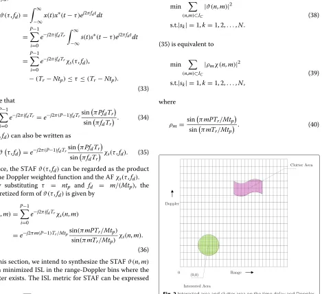
Interested and clutter areas are depicted on the dis-cretized time delay and Doppler frequency shift plane, respectively, in Fig. 2. Without loss of generality, the cen-ter of the incen-terested area can be assumed to be the origin of the range-Doppler plane. This means that the matched filter and MTD processing response of clutter returns depend on the difference of its time delay and Doppler frequency shift with respect to those of the center of the interested area.
Taking into account that the synthesized waveform should have constant module, the STAF optimization problem for a MTD radar system can be summarized as
min
(n,m)⊂IC
|ϑ(n,m)|2
s.t.|sk| =1,k=1, 2,. . .,N.
(38)
(35) is equivalent to
min
(n,m)⊂IC
|ρmχ(n,m)|2
s.t.|sk| =1,k=1, 2,. . .,N,
(39)
where
ρm= sin
πmPTr/Mtp sinπmTr/Mtp
. (40)
With the derivation in the previous section, the formula-tion can also be given by
min
(n,m)⊂IC
ρms(t)HUn,ms(t)
2
+λs(t)HU0,0s(t) 2
s.t.|sk| =1,k=1, 2,. . .,N.
(41)
The proposed optimization algorithm in Section 2.3 can also be used to solve this problem.
3.2 Workflow of a cognitive MTD radar
In Fig. 3, the workflow of a cognitive MTD radar is given. When the MTD radar begins to work, it utilizes some uni-modular sequences with good AF or ACF properties for transmission. Then, range-Doppler processing is carried out for information extraction. With the extracted infor-mation associated with the target and clutter, the radar
Fig. 3Workflow of a cognitive MTD radar system
system begins to synthesize the unimodular sequence by our proposed algorithm. In the next coherent process-ing interval (CPI), the MTD radar will transmit a new designed sequence. The above process is repeated and the MTD radar system can operate in a dynamic environment with cognitive capability. This framework is especially attractive for the confirmation process. Once a target has been found by a standard radar waveform, detection can be confirmed reliably by transmitting the optimized wave-form, which is matched to the operation scenario of the radar system.
4 Numerical examples
In order to verify the effectiveness of the proposed algorithms, we will present several numerical examples, including the AF synthesis, STAF synthesis, and detection performance of a cognitive MTD radar. In the following examples, we all assume that the unimodular sequence has
N = 100 subpulses with rectangular pulse-shaping. The
time duration of each subpulse istpand that of the total waveform isT = 100tp. The pulse repetition interval is Tr =10T, and the number of pulses in a CPI isP=64. In AF and STAF, the time delay axisτis normalized byTand the Doppler frequency axisf is normalized by 1/T. The convergence of the proposed algorithm will be tested by using randomly generated sequences in the initialization. In the iteration process, the parameteris set to be 10−3.
4.1 AF synthesis
Suppose that= {(τ,fd)||τ|< 0.2,|fd|< 0.01,τfd =0} is the interested area, which is near the origin but excludes
the origin on τ − fd plane. With randomly generated
sequence in the initialization, PCA is applied to minimize the ISL metric of the AF of the synthesized sequence.
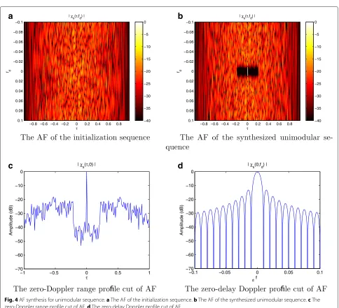
The AFs of the initialization sequence and synthesized sequence are shown in Fig. 4a,b. The AF in Fig. 4a presents high sidelobe values on the wholeτ−fdplane. The desired low sidelobes in the interested area of AF is obviously obtained in Fig. 4b. Therefore, the synthesized sequence has a good capability of separating and detecting closely spaced targets.
Figure 4c,d gives the zero-Doppler range profile cut and zero-delay Doppler profile cut of the AF in Fig. 4b. The sidelobes in the interested area is suppressed to about −40 dB in the time delay axis with|τ| < 0.2. Due to the fact that the synthesized sequence has constant modulus, the zero-delay Doppler profile cut is a sinc function.
4.2 STAF synthesis
τ fd
| χs(τ,fd) |
−0.8 −0.6 −0.4 −0.2 0 0.2 0.4 0.6 0.8 −0.1
−0.08
−0.06
−0.04
−0.02
0
0.02
0.04
0.06
0.08
0.1 −40
−35 −30 −25 −20 −15 −10 −5 0
τ fd
| χs(τ,fd) |
−0.8 −0.6 −0.4 −0.2 0 0.2 0.4 0.6 0.8 −0.1
−0.08
−0.06
−0.04
−0.02
0
0.02
0.04
0.06
0.08
0.1 −40
−35 −30 −25 −20 −15 −10 −5 0
−1 −0.5 0 0.5 1
−70 −60 −50 −40 −30 −20 −10 0
τ
| χs(τ,0) |
Amplitude (dB)
−0.1 −0.05 0 0.05 0.1
−70 −60 −50 −40 −30 −20 −10 0
f
d
| χs(0,f
d) |
Amplitude (dB)
a
b
c
d
Fig. 4AF synthesis for unimodular sequence.aThe AF of the initialization sequence.bThe AF of the synthesized unimodular sequence.cThe zero-Doppler range profile cut of AF.dThe zero-delay Doppler profile cut of AF
closely spaced targets. The specified area can be described as
1=
τ,fd τ|<0.1,fd<5×10⁻⁴
. (42)
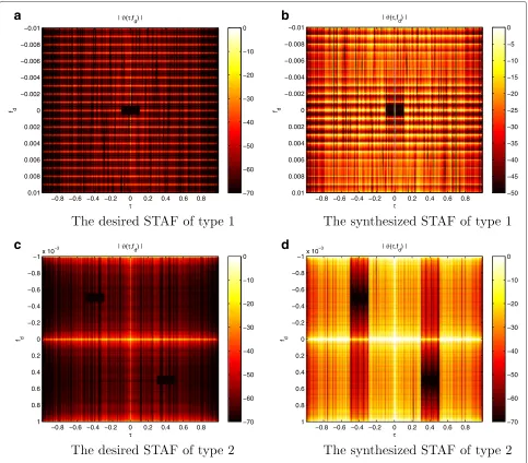
Figure 5a,b shows the desired and synthesized STAFs of the first type in log scale. The ISL of STAF in1is
mini-mized and the averaged sidelobe of the obtained sequence is suppressed to about−50 dB in Fig. 4b.
The seconde type has minimized ISL in a certain area, which is given by
2=
τ,fd |0.3<|τ|<0.5, 4×10⁻⁴<|fd|<6×10⁻⁴
. (43)
The desired and synthesized STAFs of the seconde type are plotted in Fig. 5c,d. The ISL of STAF in2is reduced
and the averaged sidelobe of the obtained sequence is suppressed to about−70 dB in Fig. 5d.
4.3 STAF synthesis in a cognitive MTD radar system
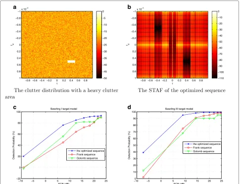
In this example, a MTD radar system is designed as a CR system. The target and clutter distributions within the radar scene should be dynamically deciphered from the received backscattered signal, and these deciphered distributions over the STAF could then be used for the proposed synthesis approach. In Fig. 6a, the clutter distri-bution on theτ −fdplane is plotted and a strong clutter block lies in
C= {(τ,fd)|0.3<|τ|<0.5,
τ
Fig. 5STAF synthesis for unimodular sequence
For ease of simulation, the clutter in every range-Doppler bin can be treated as a stationary scattering point. Hence, the whole clutter return is the superposition of all the returns from every range-Doppler scattering point.
We also assume that the target distribution can be described as
T = {(τ,fd)||τ|<0.1,|fd|<5×10⁻⁴} (45)
and consider the underlying scintillation on RCS based on different Swerling models for the moving target. The opti-mized shape of STAF is plotted in Fig. 6b, in which a low sidelobe is presented in the target and heavy clutter area.
According to the Swerling models, the RCS of a reflect-ing target can be described by the chi-square probability
a
b
c
d
Fig. 6Processing results for a cognitive MTD radar
The Swerling III model is described like Swerling I but with four degrees of freedom. The scan-to-scan fluctua-tion follows a density of probability
P(σ)= 4σ
σaverage 2
·exp −
2σ σaverage
. (47)
In Eqs. (46) and (47),σis the value of RCS, andσaverageis
the mean value of RCS.
In order to evaluate the detection performance, signal-to-clutter ratio (SCR) is defined as
SCR= PTrσ
2 average
Mtp C(τ,fd)dτdfd
, (48)
whereC(τ,fd)is the clutter distribution. In this definition, the average scattering power of the Swerling target model
is compared with the average power of all the clutter scattering points.
5 Conclusions
An algorithm was proposed to synthesize a unimodular sequence by minimizing the sidelobe values of AF in cer-tain areas on the time delay and Doppler frequency shift plane. This algorithm can be convergent theoretically and practically and has been shown to be useful for ISL mini-mization of AF and STAF. The algorithm for synthesizing the unimodular sequence with the desired AF and STAF was built in this work.
A cognitive approach to devise waveforms for a MTD radar system was also put forward in this work. With this approach, the MTD radar system can adaptively optimize the STAF of its transmit waveform by minimizing the ISL metric of the interested area and clutter area on the time delay and Doppler frequency shift plane. The numerical example shows that better detection performance can be achieved by our proposed approach.
We note further that computational efficiency of New-ton’s method was limited by matrix inversion. This algo-rithm is better for the sequence with a length no longer than 104. Therefore, in the future work, we will try to find a better approach and a computation-saving method.
Appendix
Subpulse cross ambiguity function
In order to verify the subpulse CAF in Eq. (7), we rewrite thekth andlth subpulse CAF expressions as follows:
χ(k,l)
Note that the two subsets oftoverlap with each other only whenτ = (k−l)tp+τ, with|τ| ≤ tp. The integral in Eq. (7) can be calculated in two cases.
Case 1.−tp≤τ<0
Withfdτ1, the above equation can be simplified to
χ(k,l)
Therefore, the subpulse CAF can be summarized with the following expression as
The first order derivative of ISL with respect toφcan be given by
It can be simplified to
Hence, the first item in Eq. (20) can be simplified and rewritten as
ResHU0,0s ∗U0,0ssH
=N2I.
We also note that
s∗U0,0s=1,
where1=[ 1, 1,. . ., 1]T. The second item in Eq. (20) can also be expressed as
Ims∗U0,0s Im
s∗U0,0s H=0.
With the above two equations, we can obtain the equal-ity in Eq. (20), which is expressed as
ResHU0,0s
As indicated in Section “Derivatives of ISL”, we have ∂γn,m(s)
Eq. (26) can be rewritten as
An equality can be obtained the above equation , and expressed as
This expression can be expanded by the real and imagi-nary part ofsHUn,msands∗Un,ms, and given by
The authors declare that they have no competing interests.
Acknowledgements
This work was supported by the National Natural Science Foundation of China under grant 61201367, the Natural Science Foundation of Jiangsu Province under grant BK2012382, the Aeronautical Science Foundation of China under grant 20142052019, the Fundamental Research Funds for Central Universities under grant NS2016042, and the Cooperative Innovation Foundation Project in Jiangsu Province under grant BY2014003-5.
Received: 22 May 2015 Accepted: 17 February 2016
References
1. S Haykin, Cognitive radar: a way of the future. IEEE Signal Process. Mag.
23(1), 30–40 (2006)
2. PG Grieve, JR Guerci, Optimum matched illumination reception radar. U.S. Patent S517552 (1992)
3. SU Pillai, HS OH, DC Youla, JR Guerci, Optimum transmit-receiver design in the presence of signal-dependent interference and channel noise. IEEE Trans. Inf. Theory.46(2), 577–584 (2000)
4. MR Bell, Information theory and radar waveform. IEEE Trans. Inf. Theory.
39(5), 1578–1597 (1993)
5. S A De Maio, Y De Nicola, ZQ Huang, S Luo, Zhang, Design of phase codes for radar performance optimization with a similarity constraint. IEEE Trans. Signal Process.57(2), 30–40 (2009)
6. M Skolnik,Radar Handbook, 3rd ed. (McGraw Hill, New York, 2008) 7. N Levanon, E Mozeson,Radar Signals. (NY, Wiley, 2004)
8. N Zhang, SW Golomb, Polyphase sequence with low autocorrelations. IEEE Trans. Inf. Theory.39(3), 1085–1089 (1993)
10. CD Groot, D Wurtz, KH Hoffmann. Low autocorrelation binary sequences: exact enumeration and optimization by evolutionary
strategies.Optimization.23(4), 369–384 (1992)
11. HD Schotten, HD Luke, On the search for low correlated binary sequences. Int. J. Electron. Commun.59(2), 67–78 (2005)
12. S Mertens, Exhaustive search for low-autocorrelation binary sequences. J. Phys. A.29, 473–481 (1996)
13. P Stocia, H He, J Li, New algorithms for designing unimodular sequences with good correlation properties. IEEE Trans. Signal Process.57(4), 1415–1425 (2009)
14. J Li, P Stoica, X Zheng, Signal synthesis and receiver design for MIMO radar imaging. IEEE Trans. Signal Process.56(8), 3959–3968 (2008) 15. M Soltanalian, P Stoica, Computational design of sequences with good
correlation properties. IEEE Trans. Signal Process.60(5), 2180–2193 (2012) 16. P Stoica, H He, J Li, On designing sequences with impulse-like periodic
correlation. IEEE Trans. Signal Process. Lett.16(8), 703–706 (2009) 17. M Soltanalian, P Stoica, Designing unimodular codes via quadratic
optimization is not always hard. IEEE Trans. Signal Process.57(6), 1221–1234 (2009)
18. S Sussman, Least-square synthesis of radar ambiguity functions. IEEE Trans. Inf. Theory.8(3), 246–254 (1962)
19. JD Wolf, GM Lee, CE Suyo, Radar waveform synthesis by mean-square optimization techniques. IEEE Trans. on Aero. Elec. Sys.5(4), 611–619 (1968)
20. I Gladkova, D Chebanov, inInternational Conference on Radar Systems, Toulouse. On the synthesis problem for a waveform having a nearly ideal ambiguity functions, (France, 2004), pp. 1–5
21. YI Abramovich, BG Danilov, AN Meleshkevich, Application of integer programming to problems of ambiguity function optimization. Radio Eng. Elect. Phys.22(5), 48–52 (1977)
22. H He, P Stocia, inAcoustics, Speech and Signal Processing (ICASSP) 2011 IEEE International Conference on. On synthesizing cross ambiguity functions, (Prague, 2011), pp. 3536–3539
23. A Aubry, A De Maio, B Jiang, S Zhang, Ambiguity function shaping for cognitive radar via complex quartic optimization. IEEE Trans. Signal Process.61(22), 5603–5619 (2013)
24. S Boyd, L Vandenberghe,Convex Optimization. (Cambridge Univ. Press, Cambridge, 2004)
25. B Chen, S He, Z Li, S Zhang, Maximum block improvement and polynomial optimization. SIAM J. Optimiz.22(11), 87–107 (2012) 26. M Soltanalian, P Stoica, Designing unimodular codes via quadratic
optimization. IEEE Trans. Signal Process.62(5), 1221–1234 (2014) 27. JR Guerci,Cognitive Radar, The Knowledge-Aided Fully Adaptive Approach.
(Artech House, Norwood, MA, 2010)
Submit your manuscript to a
journal and benefi t from:
7Convenient online submission
7Rigorous peer review
7Immediate publication on acceptance
7Open access: articles freely available online
7High visibility within the fi eld
7Retaining the copyright to your article