R E S E A R C H
Open Access
Audio visual speech source separation via
improved context dependent association
model
Alireza Kazemi
*, Reza Boostani and Fariborz Sobhanmanesh
Abstract
In this paper, we exploit the non-linear relation between a speech source and its associated lip video as a source of extra information to propose an improved audio-visual speech source separation (AVSS) algorithm. The audio-visual association is modeled using a neural associator which estimates the visual lip parameters from a temporal context of acoustic observation frames. We define an objective function based on mean square error (MSE) measure between estimated and target visual parameters.
This function is minimized for estimation of the de-mixing vector/filters to separate the relevant source from linear instantaneous or time-domain convolutive mixtures. We have also proposed a hybrid criterion which uses AV coherency together with kurtosis as a non-Gaussianity measure. Experimental results are presented and compared in terms of visually relevant speech detection accuracy and output signal-to-interference ratio (SIR) of source separation. The suggested audio-visual model significantly improves relevant speech classification accuracy compared to existing GMM-based model and the proposed AVSS algorithm improves the speech separation quality compared to reference ICA- and AVSS-based methods.
Keywords: Audio-visual speech source separation; Bimodal coherency; Blind source separation; Independent component analysis
1 Introduction
Audio-visual speech source separation (AVSS) is a grow-ing field of research that is developed in recent years. It is derived from mixing audio-visual speech processing (AVSP) and blind source separation (BSS) techniques.
Speech is originally a bimodal audio-visual process. Per-ceptual studies on human audition have revealed that visual modality has effective contributions in speech intel-ligibility [1], perception [2] and detection [3] especially in the noisy and multi-source (cocktail party) situations. According to the McGurk-McDonald effect [4] (that is, sensing the auditory part of a phonetic sound with visual part of another one, results in illusion of perception of a third one), it is evident that there is an early stage inter-action between audio and visual stimuli in the brain. This is confirmed in [5] that early integration of audio and
*Correspondence: [email protected]
CSE&IT Department, Electrical and Computer Engineering School, Shiraz University, Molla-Sadra, 71348-51154 Shiraz, Iran
visual modalities can help in the identification and hence enhancement of speech in noisy environment. The perfor-mance of automatic speech processing systems degrades drastically in the presence of noise or other acoustic sources. Thus, researchers have tried to incorporate visual modality to automatic speech processing systems upon the perceptual findings.
Both audio and visual modalities of speech originate from gestures and dynamics of articulators along the speaker’s vocal tract. Hence, there is an intrinsic rela-tion between these two speech cues. Although among all articulators, just the lip and, partially, jaws are visually observable. This partial observation bears a stochastic but exploitable relation between audio and visual cues.
It is inspiring to consider AV relation as two coher-ent and complemcoher-entary componcoher-ents. In the automatic speech processing community, there has been early noti-fication and interest (since 1984 [6]) for exploiting the complementary (orthogonal) portion of AV information
prior to its coherent (non-orthogonal) portion. The com-plementary information of AV data is truly adopted in audio-visual speech recognition (AVSR) in either of early-(feature), middle- (model), or late- (decoding) stage fusion schemes to enhance robustness against acoustic distor-tions. In recent years (since 2001 [7]), researchers have proposed methods based on exploiting the coherent com-ponent of AV processes for applicable tasks like speech enhancement [7-9], acoustic feature enhancement [10], visual voice activity detection (VVAD) [11], and AV source separation (AVSS) [11-24].
In [12], a statistical AV model based on Gaussian mix-ture models (GMMs) is presented for measuring the coherency of audio and its corresponding video and is used for extracting speech of interest from instantaneous squared mixtures on a simple French logatoms AV corpus. They have extended their method in [14] and assessed it on a more general sentence corpus and also for degen-erate mixtures. Wang et al. [15] have exploited a sim-ilar GMM model (but using different AV features) as a penalty term for solving convolutive mixtures. That method seems to be inefficient because it should con-vert the separating system from frequency to time domain repeatedly. Rajaram et al. [13] have incorporated visual information in a Bayesian AVSS for separation of two-channel noisy mixtures. Their method adopts a Kalman filter with additional independence constraint between the states (sources). Rivet et al. [16] have adopted the AV coherency of speech (measured by a trained log-Rayleigh distribution) for resolving the permutation indeterminacy in the frequency domain separation of convolutive mix-tures. They have also proposed another method [11] for convolutive AVSS based on developing a VVAD and using it in a geometric separation algorithm using sparse source assumption.
Sigg et al. in a pioneering work [17] have proposed a single microphone AVSS method by developing a non-negative sparse canonical correlation analysis (NS-CCA) algorithm. Their method jointly separates audio signals and localizes their corresponding visual sources. Follow-ing them, Casanovas and Monaci et al. [18-21] have pro-posed single microphone AV separation and localization methods by sparse and redundant atomic representation of AV signals. They use cross-modal correlations between AV atoms as similarity measure to cluster visual atoms for localizing visual sources and then separating audio signals. Liang et al. [22] have incorporated visual localization to improve the fast independent vector analysis (FastIVA) as a frequency domain convolutive method. They use loca-tion of sources for smart initializaloca-tion of FastIVA to solve its block permutation. Liu et al. [23] have proposed an AV dictionary learning method (AVDL) and have used it for AV-BSS via bimodal sparse coding to estimate time-frequency (TF) masks.
Khan et al. [24] have proposed a video-aided separation method for two-channel reverberant recordings which estimates direction of sources via visual localization to be used in probabilistic models which are refined using EM algorithm and evaluated at discrete TF points to generate separating masks.
In this paper, we develop a visually informed speech source separation algorithm called MLP-AVSS which con-siders temporal dependency between consecutive AV frames. We have suggested to model AV coherency using a multi-layer perceptron (MLP) for AV association. This model with lower number of parameters can capture AV coherency significantly better relative to the GMM AV model of [12,14,15]. We have also proposed a hybrid measure of kurtosis and visual coherency and based on that a time domain convolutive AVSS algorithm. We have assessed quality of suggested AV model and its induced AVSS methods on two discrete (alpha-digits) and contin-uous (poet-verses) audio-visual corpora. The former is a corpus of Persian and English alpha digits and the later is a corpus of poem verses from about 20 Persian poets.
The rest of this paper is organized as follows: In Section 2, we briefly review BSS and AVSP background and then focus on the relevant AVSS work. Section 3 illustrates the proposed MLP-based AV model and AVSS algorithm. Section 3.3 presents a hybrid AV coherent and independent criterion, and based on that, we move toward a time-domain convolutive extension. In Section 4, audio-visual materials including AV corpus, parametrization and modeling procedures is considered. In Section 5, experi-mental set-up and the experiexperi-mental results are illustrated and analyzed. Finally, the paper is concluded in Section 6.
2 Background review
AVSS has emerged from mixing BSS and audio-visual speech processing techniques [16]. In this section, after a brief review of BSS and AV speech processing back-ground, we explain the speech separation in terms of standard source separation problem and then discuss the suggested AV separation approach as an improved solu-tion for this problem.
2.1 Blind source separation problem
that is estimation of unmixed signals y(t) = B(t)x(t)
from mixed signalsxusing an unknown de-mixing matrix Bsuch that they are as similar as possible to unknown sourcess.
In (1), both sourcess(t)and the mixing processA(t)are considered non-stationary in time. In speech processing, sources (i.e. speech signals) are naturally non-stationary since (i) phonemes (and even sub-phonemes) have dif-ferent waveform statistics and (ii) a speaker may either speak or be silent over the time. Also, the mixing model may be non-stationary in time because speakers may have motion relative to sensors (microphones). It is hard to solve the problem in this case; however, if sources and mixture can be considered piecewise stationary, a solution is to divide signals to batches and solve the BSS on each batch separately:
xτ(t)=Aτsτ(t) yτ(t)=Bτxτ(t)
(2)
where τ is the batch index iterating over all batches of the signals. In this case, the mixing and de-mixing mod-els (Aτ,Bτ) are time invariant during each batch. Another
solution is to consider adaptive source separation tech-niques which is beyond the scope of this paper.
Independent component analysis (ICA) is the most well-known family of solutions for BSS problems in which algorithms such as Infomax [25], FastICA [26] and JADE [27] (to name famous ones) try to estimate sources by adopting the statistical independence assumption. The solution of most ICA algorithms is based on optimizing their specific objective functions J(B;x) which measure the independence via different orders of signal’s statistics. De-mixing matrix is then estimated by:
Bτ =argmin B
{J(B;xτ)} (3)
2.2 Audio-visual speech processing
Before explaining AV source separation methods, it is nec-essary to review some issues in AV speech processing which also inherently arises in AV source separation:
• The speech signal and lip video are non-stationary in time.
• The rate of speech samples and video frames is significantly different. In this study, the speech signal is recorded byFs=16, 000Hz while the video frame rate isFr=30fps.
• Speech signal and video frames have large numbers of samples (pixels) containing sparse information. This prevents creating audio-visual models directly from these signals.
To cope with first two issues, in most speech process-ing problems, speech is processed frame-wise with frames
of 20−30 ms length where speech signal can be consid-ered stationary. In AV speech processing, it is convenient to choose speech frame length such that audio and video frame rates are equal.
For handling the third issue, the routine solution is to extract compact and informative acoustic and visual fea-tures from speech and video frames such that each frame is represented with a few number of parameters. Frame-wise processing of speech is practical in most speech pro-cessing tasks, but the amount of speech signal in a single frame may be insufficient for source separation algorithms to perform accurately. Hence, a couple of consecutive frames must be used in each batchτ.
2.3 Audio-visual source separation
Consider problem of speech source separation in the case of instantaneous mixture of Equation (2). Most solutions (including ICA-based ones) have two major drawbacks which limit their applicability. The major problem is that ICA-based methods can estimate sources just up to a scale Dand permutationP
yτ(t)=DτPτsˆτ(t) (4)
that is signal’s amplitude gain and their order cannot be determined using these algorithms. The permutation of estimated sources may also change within consecutive frames, because sources are non-stationary in time and space. Having true or at least stable ordering of sources is crucial in most automatic speech processing applications. Furthermore, ICA-based methods do not consider or per-form weakly in case of noisy and degenerate mixtures (i.e., mixtures withM<N).
Incorporation of visual modality of speech as a source of extra information, can help to solve these problems. The permutation problem can be simply resolved and enhancement in the separation performance is gained in regular and degenerate mixtures.
Most AVSS algorithms work based on maximization of AV coherency between unmixed signalsyand their cor-responding video streams. It is shown in [12] that given coarse spectral envelope of sources, one can solve a system of equations for calculation of de-mixing matrix in regu-lar mixtures. Moreover there exists a stochastic coherent relation between the speech spectral envelope and the lip visual features [9,12]. These two facts have guided researchers toward capturing AV relation using different models and adopt it for AVSS tasks.
In [12] and [14], authors have proposed a joint statistical distributionpav(S,V)as an AV model which measures the
coherency between the acoustic spectral (S) and lip visual (V) features of the speech in each frame. The distribution
Suppose that one of sources, says1, is a speech signal for which we have a video feature streamV1extracted from
the corresponding speaker’s lip region. Then, the AVSS algorithm of [12,14] tries to estimate the first row of de-mixing matrixB1for which the outputy1=B1xproduces
spectral featuresY1as coherent as possible to the video featuresV1. This can be done by minimizing the AV inco-herency score of the following AV model which is defined on each AV framek:
MGMM(Yk1,Vk1)= −log(p(Yk1,Vk1)) (5)
However, due to the viseme-phoneme ambiguity problem [28,29], it is possible that video featuresV1in some frames
be associated to many spectral configurations. Hence, the single frame criterion (5) will result in very poor separa-tion. Consequently, they have proposed a batch-wise AV criterion which integrates joint log-likelihood on all theT
frames of current batchτ:
Jav GMM(B;xτ,Vτ1)= T
k=1
MGMM(Yτ1(k),Vτ1(k)) (6)
The summation in (6) is based on the assumption that AV frames in consecutive frames are independent from each other.
In the rest of this text unless mentioned otherwise, we always consider a single row de-mixing vector denoted by
B corresponding to a single visual stream. For the sake of brevity we omit the superscript (.)1of variables. It is clear that in case of existence of multiple video streams corresponding to more than one speech sources, all the described methods can be repeated for each video stream.
3 Audio-visual speech source separation using MLP AV modeling
Here, a method is proposed for separation of the source of interestsfromMmixed signalsx. The goal is to estimate
Bsuch thaty = Bxbe similar as possible to the original sources.s is unknown but we have the visual streamV corresponding to it, we can estimate Bsuch thatVˆ (the estimated visual stream corresponding toy), be as close as possible toV.
A problem with objective function (6) of [12] and [14] is that it does not efficiently model the non-linear AV rela-tion (as is discussed later in this secrela-tion). Also it considers independence (i.i.d) assumption in modeling relation of consequent AV frames. We suggest to improve the AV criterion via more realistic assumptions.
Consider the batch-wise separation problem of equation (2) where every batchτ consists ofT frames. It is ideal to model and measure the degree of AV coherency on the joint whole sequences of audioSτ(1 :T) and visual
Vτ(1 :T)frames considering the true dependency among
the variables. LetMIDL(Sτ,Vτ)be such an ideal model
which measures the degree of incoherency between AV streams. Then, the de-mixing vectorBτmay be estimated by minimizing the ideal AV criterionJav IDL(B;xτ,Vτ) =
MIDL(Yτ,Vτ).
However, training such an ideal model is not practical due to the need for large amount of AV training data and also due to its train and optimization complexity. Hence, considering some relaxation assumptions which factor-izes the model to a combination of some reusable factor(s) is inevitable. The independent and identically distributed (i.i.d) assumption considered in GMM model of (6) is not a fit assumption for modeling the speech AV streams. Thus we propose an enhanced model with a weaker indepen-dence assumption. Instead of considering absolute inde-pendence between AV frames, we consider a conditional independence assumption that is the coherency of an AV frame can be estimated independent of other frames given a context of a few (K) neighbor frames.
An extension of pav(S,V) to model joint probability
density function (PDF) of K consecutive AV frames is not efficient. GMM and Gaussian distributions with full covariance matrices are not suitable for modeling large dimensional random vectors since the number of free parameters of these models is of orderO(d2) relative to the dimensiondof input random vectors. Increasing the input dimension by concatenation of K AV frames will result in a very complex model with huge number of free parameters that are not used effectively.
We propose to use a MLP instead of GMM and mean square error (MSE) criterion instead of negative log prob-ability (as incoherency measure) to provide an enhanced AV criterion. The number of free parameters of an MLP with narrow hidden layer(s) is of orderO(di+do)relative
to dimensions di anddo of its input and output.
More-over, MLP makes efficient use of its free parameters in learning non-linear AV relation, according to its hierar-chical structure compared to shallow and wide structure of GMM. MLP, like GMM, is differentiable relative to its input. Hence, an objective function defined based on MLP can be optimized with fast convergence using derivative based algorithms.
3.1 MLP audio visual model
Having acoustic and visual streams of feature frames S andV extracted from pairs of corresponding AV signals
as output, to approximate the AV mappingh(.). The MLP-based AV incoherency model MMLP is then defined as
MMLP(Ye(k),V(k))= V(k)−h(Ye(k))2 (7) 3.2 Audio visual source separation algorithm
To compensate for phoneme-viseme ambiguity, the MLP model must be used in a batch-wise manner. Hence, as in (6), AV criterion is boosted by integrating incoherency scores ofTframes in each batchτ:
Beside the difference in negative log probability and mean square error, another difference between AV objective functions (6) and (8) is the form of independence assump-tion in measuring the incoherency. The former considers absolute independence (i.e., i.i.d.) between the frames while the later assumes conditional independence.
For each batchτ of mixed signals and having a visual streamVτ corresponding to one of the speech sources,
the goal of separation is to find the de-mixing vectorBτ. As in (3), this can be achieved by minimizing AV contrast function:
Bτ =argmin
B {
Jav MLP(B;xτ,Vτ)} (9)
This can be done via first- or second-order derivative-based optimization methods. For example, using the delta rule of gradient decent, we have
Bτ(i)=Bτ(i−1)−η∂Jav MLP(B;xτ,Vτ)
∂B (10)
where η is the learning rate which either is set to a fixed small number or is adjusted using line search. The gradient ofJav MLP with respect to B(omitting constant
parameters for brevity) is calculated as:
∂Jav MLP(B)
In the last summation, the first term is gradient of MLP AV model with respect to its input acoustic contextYe(k)
and the second term is gradient of acoustic features with respect to the de-mixing modelB. Gradient-based algo-rithm iteratively minimizes the problem (9). Starting from an initial pointBτ(0), at each iterationi, the gradient (11) is calculated, and using (10) or a quasi-Newton method, the improved de-mixing vectorBτ(i+1)is estimated. This
continues until the change in the norm ofBτorJav MLP(Bτ)
becomes smaller than a pre-defined threshold.
Since the AV contrast function is not convex, the opti-mization algorithm is prune to local minima. Thus, selec-tion of a good initializaselec-tion pointBτ(0)is important. A simple option may be to start from random initial points multiple times. Most ICA algorithms (including FastICA [26] and JADE [27]) start from uncorrelated or white sig-nals. Thus, another suggestion for initial pointBτ(0)is to apply PCA on mixed signalsxτof the current batchτ and,
among eigenvectors, select a vectorWthat produces a sig-naly=Wxwhich is most coherent with the visual stream
Vτand use it as the initial pointBτ(0).
Both the proposed and existing AVSS algorithms do not suffer from the permutation ambiguity due to the informed nature of AV contrast functions. Nevertheless, the scale indeterminacy should be considered in design of AV contrast function and optimization method. AV model must be invariant regarding a constant gain to audio sig-nal; that is, it must comply with the following constraint:
Jav MLP(αB;x,V)=Jav MLP(B;x,V) (12)
3.3 AVSS using AV coherency and independence criterion Although the existing and the proposed AV coherency-based methods provide improvements in speech source separation, but these methods totally neglect the useful constraint of independence of the sources. The statistical independence criteria used by ICA methods has been suc-cessful in many BSS methods. In this section, we consider the benefit of using AV coherency and statistical inde-pendence together to gain more enhancement in speech source separation.
3.3.1 Video-selected independent component
Due to permutation indeterminacy (4), separated signals from ICA methods can not directly be used in real speech processing applications. Further, to calculate output signal to interference ratio (SIR) performance of ICA methods, it is required to know which of the de-mixed signals is related to the source of interest.
3.3.2 Hybrid video coherent and independent component analysis
Contrary to the previous section where a sequential and loose combination of ICA and AV coherency model was considered, here we propose a parallel and tight com-bination using a hybrid criterion which benefits from normalized kurtosis as a statistical independence measure in conjunction with the AV coherency measure.
Kurtosis and neg-entropy are used in ICA methods such as FastICA [26] which work by maximizing the non-Gaussianity. The first kurtosis-based BSS method was presented in [30] to separate sources via deflation. It starts by pre-whitening the observed signals. Then the first source is estimated asy = Bxfrom white observations xusing a normalized de-mixing vectorB. It is estimated by maximizing the kurtosis of y, defined as kurt(y) = E{y4} − 3(E{y2})2 (for zero-mean y) that is done via a gradient-like method. The kurtosis value is zero for Gaus-sian signals while it is positive or negative for signals with super- or sub-Gaussian distributions. If both super- and sub-Gaussian sources are expected to be extracted, then absolute or squared value of kurtosis must be maximized. In [26], Hyvarinen et al. proposed a fast fixed point algorithm for solving the constrained optimization of the kurtosis and a family of other neg-entropy-based criteria under the normalized constraint forBwhich resulted in the well-known FastICA algorithm.
The reason for pre-whitening and forcing normalized constraint onBis that the kurtosis is not scale invariant (i.e. kurt(αy)=α4kurt(y)) and hence it depends both on energy and non-gaussianity of the signal. In [31] and [32] normalized kurtosis defined as
kurtn(y)=
kurt(y)
(E{y2})2 (13)
is adopted on direct observations. The normalized kurto-sis is scale invariant (i.e. kurtn(αy) = kurtn(y),∀α = 0).
Hence, it eliminates the necessity for pre-whitening and normalization constraint on the de-mixing vectorB. To gain further improvement, we propose a hybrid criterion based on combination of the AV criterion (8) and the normalized kurtosis:
Jav ICA(B;xτ,Vτ)=Jav MLP(B;xτ,Vτ)−λkurtn(Bxτ)
(14)
where λ is a positive regularization coefficient. Since speech signal is known to have super-Gaussian distribu-tion [33,34], the kurtosis term is added with negative sign such that it tends to be maximized during minimization of (14).
It must be noted that, in short time durations, the kurtosis score is not robust and does not provide
signif-icant improvement. Thus, (14) is developed to be used for convolutive case where quite large batches are con-sidered. In fact, our tests revealed that for small batch sizes used in instantaneous mixtures, the performance of the AV method using kurtosis penalty does not improve compared to the pure AV method.
3.4 Toward a time domain AVSS for convolutive mixtures Here, we consider convolutive mixtures defined by a MIMO system ofM×NFIR filtersA=[Aij]. The mixture
system can be represented in the the Z-domain as
X(z)=A(z)S(z) (15)
We are interested in estimation of a 1×M row vector
B(z)of de-mixing FIR filters which separates the source
S1(z) = B(z)X(z)that is as coherent as possible with the video streamV1. In [31], a time domain algorithm based on maximizing (normalized) kurtosis is presented which deflates sources one-by-one using non-causal two-sided FIR filters. We consider it as our baseline audio-only con-volutive method in our experiments. Following [35], we define an embedded matrix notation which transforms the convoltive mixture (15) to an equivalent instantaneous mixture. Letx(n)be an embedded column vector defined in each time stepnas:
x(n)=x1(n+L),· · ·,x1(n−L),· · ·,xM(n+L),· · ·,
xM(n−L)T
(16)
It contains M(2L+1) observation samples and using it the convolutive de-mixing process for separation of signal
s1 can be expressed asy(n) = Bx(n) whereBis a row vector containing coefficients ofMde-mixing FIR filters each one having 2L+1 taps. This is just an instantaneous mixture withM(2L+1)virtual (embedded) observations and can be solved using the kurtosis-based method of [31] or using our proposed criteria (14).
As a final note, it should be mentioned that the refer-ence method of [31], can estimate de-mixing filters up to a scale and time delay. Thus, a cross-correlation step is nec-essary to fix the possible delay of filters. For further details please refer to [31]. When dealing with convolutive mix-tures, it is necessary to calculate the objective scores on longer segments of signals since there are larger number of parameters to estimate.
4 Audio-visual data and models
4.1 Audio-visual data
To evaluate the proposed algorithm, we have recorded a proper AV corpora which is comparable in (size and com-plexity) to the corpora used in former research. Unlike [11,12], we have not used lip blue make-ups in data recordings since we do not need lip segmentation for extraction of geometric features such as width and height. Instead, the pixel gray values of speaker’s mouth region are used to extract the visual parameters. We have recorded two different types of corpora. The first corpus consists of discrete Persian and English alphabet and digits with a vocabulary size of 78 words (32 + 10 Persian and 26 + 10 English alpha-digits). The second corpus is continuous and consists of 140 verses of Persian poets. Both corpora are uttered by a male speaker. Each corpus is recorded two times. The first recording is used for training AV models and the second recording is used in evaluation phase.
In each recording, camera is focused on the speaker’s mouth and a video stream together with a mono audio stream is recorded. The raw video is captured in VGA size, true-color format (RGB 24 bits/pixel 8 bits/color) and at the frame rate ofFr 30fpsand audio is recorded using
16 bits/sample and at sampling frequency of Fs =
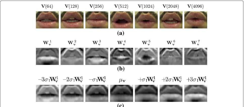
16, 000 Hz. The final mouth region video used in the experiments of this paper, is stored in true-color 160× 120 resolution frames. Sample lip region images from audio-visual corpus are shown in Figure 1a.
4.2 Audio and video parameter extraction
As discussed before, speech signal and lip image frames are high-dimensional data with sparse information related
to our task. Thus, parametrizing audio and visual frames to compact vectors is necessary. Here, we clarify the methods for audio and visual feature extraction.
4.2.1 Audio parametrization
In most speech processing tasks, log spectral envelope (cepstral) features are utilized as effective features. We use PCA projected (whitened) log power spectral den-sity for the speech frames parametrization. Let Y(k) = f(y(k)) = f(Bx(k)) be acoustic feature mapping func-tion which extractskaspectral envelope featuresY from every framekof the estimated signaly. In practice, audio featuresY are extracted from the spectrumY of the de-mixed signaly. Since for the separation algorithm we need to efficiently calculate Y and its derivative with respect to the de-mixing vectorB, we define an alternate audio feature extractor functionF(.) which efficiently extracts features from the frequency domain representation ofy:
Y(k)=F(Y(k))=F(BX(k)) (17) whereY =F{y}andX=F{x}are the fast Fourier trans-form (FFT) ofyandx, respectively. In the right-hand side (RHS) of (17), we have used the linear property of FFT that is, for every matrixB,F{Bx} = BF{x}. Thus, we can pre-calculateXusing FFT and then for any value of the de-mixing vectorBthe frequency domain de-mixed signal
Y (and its derivative) can be efficiently obtained without FFT recalculation. As in [14], we have consideredn=32 spectral coefficients in the range [ 0, 5, 000]HzasY(k)for each frame. Power spectrum vector of each frame Y(k)
Figure 1Visual modality: data and parametrization.(a)Shows some frames (k= 64, 128, 256, 512, 1024, 2048 and 4096) of visual inputV(k) from train set of the poet verses corpus.(b)Shows top seven eigen-lipsWi
vwith largest eigenvalues.(c)Demonstrates the effect of varying the
average image of all frames in the direction of the major principal axis (W1
v) with−3,−2,−1, 0, 1, 2 and 3 times of square root of the corresponding
is then defined asPSY(k) = [Y(k)⊗Y∗(k)]T, where⊗,
(.)∗ and(.)T are element-wise product, complex conju-gation and transpose operators. Although the lip and the speech spectral envelope shapes are correlated, but there is not any meaningful relation between the lip shape and speech loudness (energy). Thus, it is important to normal-ize the energy of power spectrum in each frame resulting in power spectral density (PSD). The PSD coefficients are then converted to decibels (dB) using logarithm
log PSDY(k)=log
Finally, whitening is applied to reduce the dimension of acoustic feature vectors to ka elements. The
acous-tic whitening matrixWa ∈ Rn×kais computed from the
train data using eigen-value decomposition and is used to project train and test feature vectors toka-element
com-pact spectral acoustic vectors. The overall acoustic feature extraction functionF(Y)is defined as follows:
Y(k)=F(B;X(k))=WTalog
[(BX(k))⊗(BX(k))∗]T BX(k)2
(19)
The Jacobian of F with respect to B is derived in the Appendix in Equations 22, 23 and 24. The derived for-mulas are efficient and do not need FFT recalculation for different values ofB. It is also worth to mention that the mappingFis invariant regarding a scalar multiplica-tion (i.e.F(αB;X(k)) = F(B;X(k)),∀α = 0). A property that entails gain invariance property (12) in AV contrast functions (6) and (8).
4.2.2 Video parametrization
In previous works, such as [11,12,14], authors have used geometric lip parameters that need lip contour detection to estimate the width and height of interior lip contour. We extract holistic visual features from all pixels of the mouth region. This requires less computation and does not require contour fitting. Let functiong(.)be visual fea-ture mapping function which extracts kv visual features
from any video frame. We assume that mouth region can be extracted from video using detection and tracking algo-rithms. There exists efficient parametric head tracking algorithms such as [36] which can be adopted for this task. The corpus used in this paper simply provides lip region in each frame. To extract kv visual features, the mouth
region of each frame is shrunk to 32 × 24 pixels and then reshaped to 768× 1 image vectors. Finally, a PCA transform is applied to extract visual features. The PCA matrixWv∈R768×kvis computed from the train data and
is used to project train and test mouth region images to
kv-element visual parameter vectors. Figure 1b represents top major eigen-vectors (eigen-lips) in order.
The overall visual feature extraction function is defined as normalized projected gray values of mouth region:
V(k)= g(V(k))= QTvWTvV(k), whereQvis the diagonal
scaling matrix calculated from square root of correspond-ing eigen-values.
To assess and understand the virtue of visual features, a simple yet insightful simulation is illustrated in Figure 1c. In PCA, the eigenvector with largest eigenvalue captures most of the variance of dataset. Most variance of lip images during speaking is along opening and closing of lips. Thus, it is expected that the principal eigenvector W1v will model this direction of variation. To check this, we calculated mean vectorμvof all video frames in
poet-verses train corpus and illustrated its variations along the principal eigenvectorW1v with negative and positive integer multiplies of square root of corresponding eigen-value σ1. Results presented in Figure 1c show that this
has resulted in synthesized opening and closing of lip images.
Figure 2a,c demonstrates two segments of discrete and continuous speech from alpha-digits and poet-verses cor-pora and Figure 2b,d shows the corresponding first visual feature (before normalization). In discrete or slow speech, first visual feature shows a quasi-periodic shape corre-sponding to the periodic lip opening and closing. In con-tinuous or fast speech, lip opening and closing is partial and this makes it more complex.
4.3 Building audio-visual models
In addition to estimation of transformsWaandWv, that
are part of the AV feature mapping functionsf(.)andg(.), the train set of each corpus is used to learn the AV mod-els. The training set consists of synchronous sequences of AV pairs(S(k),V(k))extracted from the raw AV data. For training models with K > 1, first, the embedded acoustic stream Se is formed by K-fold embedding of
frames of acoustic stream S. Instead of stacking the K
frames of context, it is better to stack the center frame together with temporal difference of other frames. This reduces the redundancy in the embedded vector. Then, embedded pairs (Se(k),V(k))are used to train models. Both GMM and MLP models are trained with differ-ent context sizes for fair comparison. But as experimen-tal results of Section 5.1 shows, GMM degrades with
K>1.
For training GMM models, AV components of each pair are concatenated and considered as samples of joint PDF
pav(., .). These samples are used for estimation of GMM
parameters using maximum likelihood via expectation maximization (EM) algorithm [37]. GMM distributions with various configuration of parameters (ka,kv,NM,K)
Figure 2Sample segments of speech signal and first visual feature corresponding to them.(a,c)discrete and continuous speech segments from alpha-digits and poet-verses corpora.(b,d)First visual feature corresponding to (a,c).
GMM distribution is trained 20 times using EM with ran-dom initialization and the best model is selected based on a validation subset of training data. Regularization by adding a small positive number in range [ 10−10, 10−2] to
diagonal elements of covariance matrices was adopted to hold positive definiteness where necessary (specially for models with larger random vector dimensions).
MLP AV models are also trained on AV pairs
(Se(k),V(k)) with Se(k) as input and V(k) as output.
MSE criterion between true and estimated outputsV(k)
andVˆ(k) is used as the performance measure in train-ing. This is the same criterion as what is used in contrast function (8). Networks were trained using the Levenberg-Marquardt algorithm [38] and via early stopping based on validation subset to avoid over-fit. As for GMM, MLP models with various configuration of parameters (ka,kv,
NH,K) are trained. To avoid local minima in training, each model is trained 20 times with random initialization and the best model is selected based on the validation subset.
5 Experiments and results
For evaluation of the proposed method, we have con-ducted four sets of experiments at different stages. First fitness of AV models in capturing AV coherency is evalu-ated with some initial experiments providing enough data for hyper-parameter selection of models. Then, multiple source separation experiments on regular (N × N) and degenerate (M×N,M<N) cases are conducted to com-pare performance of proposed MLP-based AVSS method with GMM-based AVSS and JADE-AV method (defined in Section 3.3.1). Finally, experiments on convolutive 2×2 mixtures with filters of different length are presented to compare performance of the audio-only and the proposed hybrid method.
training and have hyper-parameters to be selected. We should choose proper dimensions ka andkv of acoustic and visual parameters, the embedding context sizeK, the number of hidden neuronsNHof MLP and the number of
Gaussian componentsNMof GMM models. Although
val-idation scores of trained models can be used to select best GMM and MLP models, but selection of models based on their capability of discrimination between coherent and incoherent speech is more reasonable since models are aimed to be used for source separation. Furthermore, such an experiment provides insights in virtual potentials of coherency-based AVSS methods.
5.1.1 Audio-visual pure relevant source detection
In this experiment, we compare incoherency scores between a visual streamV1and two pure audio signals: a coherent signals1and an irrelevant signals2. For each frame in the test set, the signal which produces minimum incoherency score is recognized to be coherent with V1. Experiments are performed for both AV models
MGMM(S,V)(5) andMMLP(S,V) (7). For each model,
different values of hyper-parameterska∈{2, 4, 6, 8, 10, 12}, kv ∈ {2, 4, 6, 8}, NM,NH ∈ {4, 8, 12, 16, 20, 24, 28}, K ∈
{1, 2, 3, 4, 5, 6} are examined. Finally, the percent of all frames which signal s1 is truly selected is reported as classification accuracy for different values of batch sizeT. In [14], authors have evaluated the classification rate just against a single irrelevant signal which is uttered by a different male speaker. Our initial experiments revealed that classification accuracy for different irrelevant signals is variable depending on the speaker, the speech content of signal and alignment of silent parts of coherent and incoherent signals. Thus, to provide classification rates with high confidence, we conducted multiple simulations by performing coherency classification on the relevant signal s1y against six distinct speech signals for s2 and reported the average recognition rate as the performance of models.
Furthermore, it is possible that AV models, in addition to AV coherency of speech, capture some parts of AV identity of speaker. To check for this, we chose coher-ent and irrelevant speech signals both from the same speaker. As much as AV models have captured speaker identity, this provides a classification problem which is more confusing and complex for them relative to choosing irrelevant signals from different speaker(s).
Table 1 Optimal embedding context size (K) and model sizes (NMof GMM andNHof MLP)
GMM(K/NM) MLP(K/NH)
ka kv:2 4 6 8 2 4 6 8
2 1/4 1/16 1/28 1/8 4/20 4/16 4/20 6/28
4 1/24 1/24 1/24 1/20 4/20 3/16 2/24 3/16
6 1/28 1/20 1/24 1/24 4/8 2/24 3/16 2/8
8 1/8 1/8 1/28 1/28 2/20 2/16 2/28 2/16
10 1/24 1/28 1/28 1/24 2/16 2/28 2/16 2/16
12 1/8 1/16 1/20 1/20 4/4 2/16 2/20 4/8
Optimal values are selected using cross validation for different values ofka
andkv.
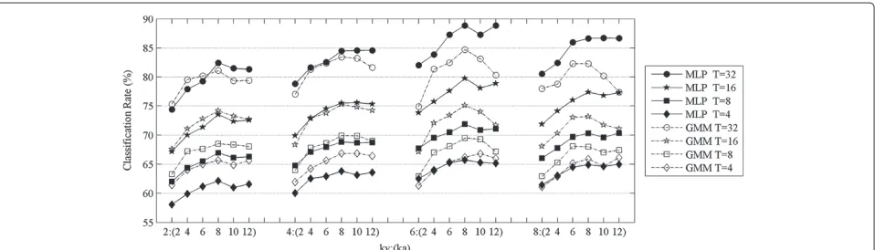
Comprehensive classification rates are presented in Figure 3 for both GMM and MLP models and for differ-ent values ofka,kvandTas free parameters. In this figure,
other parameters (NH of MLP, NM of GMM and K of
both models) are marginalized by selecting the maximum accuracy among them.
Table 1 presents optimal values for hidden (marginal-ized) parameters (NH,NMandK) of Figure 3 for different
kaandkvconfigurations in both GMM and MLP models. The common trends in classification rates of Figure 3 reveals following points:
1. Accuracy of both MLP and GMM models is enhanced by increasing the number of batch frames T, acoustic featureskaand visual featureskv. 2. Among these factors, batch sizeT has the highest
impact and this is followed byka; finally,kvhas the
lowest impact.
Comparing the trends in Figure 3 for MLP and GMM models, also reveals interesting points:
1. MLP model performs significantly better relative to GMM in various AV dimensions.
2. In lower visual dimensions (kv=2), MLP
outperforms with a10−15% gap relative to GMM model. In this case, even performance of MLP with worst condition (batch sizeT =4) is5−6% higher than GMM with best condition (batch sizeT=16). 3. In higher visual dimensions (kv=6, 8), the difference
between GMM and MLP is somewhat reduced. 4. The improvements by increasing number of features
kaandkvis bounded. Forkv>8, in MLP,kv>6in
GMM andka>8in both models, no more
significant enhancement is achieved. The model complexity increases inO(K.ka+kv)for MLP and O((K.ka+kv)2)for GMM and in some point, this
results in over-complex models for the problem (considering the amount of available training data). 5. Contrarily, improvements by increasing batch size
(T ) continues upward and may reach perfect accuracy for enough largeT values. This is because the value ofT does not change the model size while increasing it introduces more information for decision making. However, it is important to
mention that for real AVSS tasks, we cannot increase T arbitrarily. This makes the stationary assumption considered in the mixture model (2) invalid. Hence, there is a trade-off on the value ofT between the AV model accuracy and the mixing model fitness.
Finally, results of optimal K, NH andNM values
pre-sented in Table 1 reveals that
1. In variouskaandkvs, GMM always has performed
better withK=1frames in embedded context which means GMM can not capture temporal dynamics by frame embedding due to quadratic order of parameters.
2. MLP always has performed better withK=2frames (for greaterka) orK=4, 6frames (for smallerka) in embedded context showing that it can capture some temporal dynamics.
Table 2 Average input (mixed) SIRs in decibels for both corpora and for differentM×Nmixing matrices
Ch.i Alpha digits Poet verses
2×2 2×3 3×3 5×5 2×2 2×3 3×3 5×5
Ch. 1 0.6 −2.5 −3.2 −9.0 −0.7 −3.9 −4.5 −10.2
Ch. 2 −1.8 −4.8 −5.9 −8.6 −3.2 −6.1 −7.3 −9.9
Ch. 3 - - 0.4 −8.8 - - −0.9 −10.1
Ch. 4 - - - −8.2 - - - −9.4
Ch. 5 - - - −6.7 - - - −8.0
SIRs values are calculated with respect tos1(SIR(xi|s1)) and they are averaged
over all simulated input random matrices and all frames for each corpus.
3. Both GMM and MLP models exploit maximum average number of latent units inkv=6which
seems to be efficient optimal visual dimension size according to results of Figure 3.
5.1.2 Audio-visual mixed relevant source detection
Recall that classification results in Section 5.1.1 are based on comparing the incoherency scores between pure rel-evant and irrelrel-evant speech signals. This entails that AV models are well suited for selection of a clean relevant source among multiple available irrelevant signals. For example, it will perform well for relevant source selection in AV-assisted ICA-based source separation method (i.e. JADE-AV) discussed in Section 3.3.1.
In AV separation algorithms, models must provide scores for signal of relevant source which is more or less contaminated by other sources specially during first iter-ations of the optimization algorithm. Hence, a good AV model must be such that it provides decreasing inco-herency scores for increasing amounts of SIR. Therefore, we conducted another experiment to assess how well AV models comply with this property. Letξi=s1+αis2be a
mixed signal composed of sources1coherent with visual
streamV1and an irrelevant speech or acoustic signals2.
Mixed signals at different SIRs can be generated using dif-ferent values for mixing coefficientαi. We generated a set
of mixed signals ξi with SIRs in range [−5, 30] dB and
performed classification using incoherency score compar-isons between signal pairs(ξi,ξi+1)at different SIR levels. Here, the classification accuracy is defined as percent of all frames which the signal with higher SIR is selected.
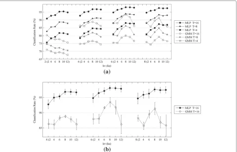
Figure 4 shows average classification accuracy measured at different SIR levels for all GMM and MLP models tested in previous experiment.
Generally, trends of Figure 4 shows similar properties as was discussed for Figure 3. The major point is that classi-fication accuracies of best models on mixed signalsξi,ξi+1
is something about 10% less relative to classification of pure relevant and irrelevant signals. Such a degradation is predictable since signalsξi andξi+1are very similar. But the interesting note is that superior models in the pure classification have approximately kept their superiority in the mixed case. This means that optimal model configu-rations which are better for classification task, may keep their position in separation task. As before MLP models are superior to GMM models but the large gap between them is somewhat reduced.
5.2 Source separation experiments
5.2.1 Separation performance criterion
In our experiments, we will simulate the mixing pro-cess using some mixing matrices. Thus, we have original source signals and it is possible to calculate the SIR of each acoustic source specially the source of interest (s1) in all mixed and de-mixed signals. Lete(si)be the energy of sourceiandxibe theithmixed signal produced by the mixing matrixA. Then SIR ofs1 in each of input-mixed observations can be calculated as
SIR(xi|s1)=10 log10(a2i1e(s1)/ N
j=2
a2ije(sj)) (20)
whereaijis the element of mixing matrix at positionsi,j.
The input SIR is useful for analysis of complexity of mixing matrices utilized in simulations. Similarly, consider Bas estimated de-mixing vector for sources1and letG=BA be the global mixing and de-mixing vector for this source. Then output SIR ofs1in estimated de-mixed signalycan be calculated as:
SIR(y|s1)=10 log10(g112e(s1)/ N
j=2
g1j2e(sj)) (21)
The output SIR criterion is widely used in performance evaluation of source separation algorithms when original source signals or mixing systems are available [39]. Since
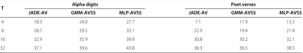
Table 3 Average output SIRs in decibels for 2×2 case
T Alpha digits Poet verses
JADE-AV GMM-AVSS MLP-AVSS JADE-AV GMM-AVSS MLP-AVSS
4 18.3 24.0 27.7 7.1 11.9 13.3
8 28.7 29.5 35.1 22.9 19.4 21.4
16 32.9 35.9 39.9 30.8 30.2 32.1
Table 4 Average output SIRs in dB for 3×3 case
T Alpha digits Poet verses
JADE-AV GMM-AVSS MLP-AVSS JADE-AV GMM-AVSS MLP-AVSS
8 18.2 19.9 23.8 11.0 9.0 10.1
16 22.8 25.3 29.1 18.8 18.2 19.8
32 27.1 28.7 31.6 25.7 25.4 26.7
in our experiments, we perform batch-wise separation, the output SIR is averaged over all batches in the test set. It is worth to mention that in convolutive mixtures, the SIRs must be calculated up to an allowed arbitrary filter-ing of the sources. This can be accomplished, usfilter-ing the decomposition method of Vincent et al. [39].
5.2.2 Separation in regular N×N mixtures
In this experiment, we consider regularN ×N mixtures with equal number of sources and sensors. Simulations are performed for mixtures of different sizesN = 2, 3, 5 and separation performance in terms of output SIR (21) is presented. Experiments are conducted on the test set of both alpha-digits (Persian and English) and poet-verses (Persian) corpora (see Section 4.1 for corpus details). Each corpus consists of a pair of synchronous audio and visual streams of frames. From each corpus, 3,000 frames are exploited in separation simulations. The audio stream from test corpus is considered as the relevant sources1
and for otherN −1 sources, speech signals of the same length are used. These speech signals are selected from a supplementary corpus recorded from other speakers with the same sampling frequency.
Since the performance of GMM- and MLP-based AVSS methods is not uniform in different mixture matrices, we have conducted Monte-Carlo (MC) simulations with 20 different random mixing matrices for each mixture size
N×N. Table 2 summarizes the average mixed input SIR of each sensor with respect tos1in various mixtures. Input SIRs are also useful in analysing the gained SIR specially in degenerate mixtures where output results is very sensitive to chosen mixing matrices. Mixing matrices are kept the same for both corpora. For each corpus and mixture size, input mean SIRs are obtained by calculating average on all the simulated random mixing matrices.
For each corpus and mixture size, speech source sep-aration using, JADE-AV, GMM-AVSS and MLP-AVSS
methods are conducted to all simulation matrices in order to estimate the de-mixing vectors. Then, the average out-put SIRs is calculated over all estimated de-mixing vectors and all batches of separated signals. Results are presented in Tables 3 (forN =2), 4 (forN =3) and 5 (forN =5). Since in this experiment, mixing matrices are squared and invertible, relatively high-output SIRs are achieved in all tested configurations. Analysis and comparison of results in terms of separation algorithms, batch integration size, mixture size and corpus reveals the following points:
Effect of discrete and continuous speech: The perfor-mance of all methods is higher on alpha-digits corpus compared to poet-verses. Alpha digits corpus is discrete and poet-verses corpus is continuous. It is obvious that continuous speech is more complex for AV modeling since lip formations are not well expressed due to speech speed (co-articulation) and also since in continuous corpus there is much number of different words and phonetic contexts which increases the phonetic complexity.
Relative separation performance of methods: In lower mixture sizes (N = 2, 3), MLP-AVSS method provides higher output SIRs relative to GMM-AVSS and both of them are superior to JADE-AV for alpha-digits corpus. In
N = 3, 5 and for poet-verses corpus, the performance enhancement gap between AVSS methods and JADE-AV is reduced. In this case, performance gain of GMM-AVSS is marginal and some times worst relative to JADE-AV. The superiority of MLP-AVSS relative to GMM-AVSS is consistent with classification accuracies of MLP and GMM-based AV models presented in Section 5.1.
Effect of batch integration time (T): The performance of all methods increases with increasing the number of frames in each batch. Increasing the integration time enhances accuracy of contrast functions (6) and (8) (see Section 5.1) and also reduces spurious local minima in the optimization landscape. For JADE-AV algorithm, in addition to improved accuracy of AV contrast, increasing
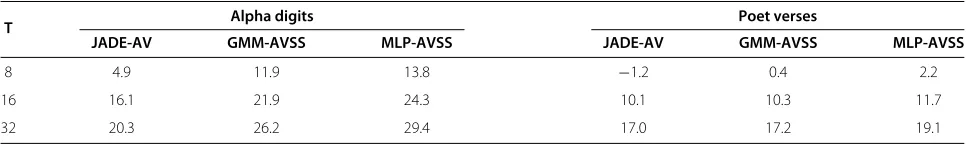
Table 5 Average output SIRs in dB for 5×5 case
T Alpha digits Poet verses
JADE-AV GMM-AVSS MLP-AVSS JADE-AV GMM-AVSS MLP-AVSS
8 4.9 11.9 13.8 −1.2 0.4 2.2
16 16.1 21.9 24.3 10.1 10.3 11.7
Table 6 Average output SIRs in dB for 2×3 case
T Alpha digits Poet verses
JADE-AV GMM-AVSS MLP-AVSS JADE-AV GMM-AVSS MLP-AVSS
16 3.9 4.7 5.9 −0.5 −0.8 1.1
32 4.1 5.2 7.4 −0.6 −0.7 2.9
64 4.5 6.5 8.9 1.6 2.8 6.7
integration time allows better estimates of higher order statistics of signals which affect separation quality of JADE algorithm. But recall that in real applications with non-stationary mixtures, there is a trade-off for increasing number of frames in each batch (see Section 5.1).
5.2.3 Separation in degenerateM×N,M<Nmixtures
In this experiment, we performed Monte Carlo simula-tions with 20 random matrices of sizeM×N = 2×3. Average mixed input SIRs of two channels on all simulated random matrices and for all test frames of each corpus is presented in the corresponding columns of Table 2. Like before, de-mixing matrices are estimated by running the proposed and baseline source separation methods. Results are presented in Table 6.
In this case, the mixing matrices are degenerate and have not exact inverse. Hence, the perfect recovery of sources is not possible and SIRs are worse relative to regular N ×N simulations. AVSS methods show slight improvements relative to JADE-AV methods. The perfor-mance of MLP-AVSS is again superior to GMM-AVSS as is predicted. In this experiment, results were highly dependent on mixing matrix. In some mixtures, output SIRs near to 10 dB were achieved while in some others negative output SIRs were observed.
5.2.4 Separation of convolutive2×2mixtures
In this experiment, we considered separation of 2×2 con-volutive mixtures using methods described in Section 3.4. We generated random mixing systems for each filter size
(2L+1)and simulated the mixtures. The separation was conducted with the same number of(2L+1)taps for each de-mixing filter. Due to the complexity of the convolutive problem, it is necessary to use large batch sizes. So we con-sidered batches of 5 s. Results in terms of output SIR are presented in Table 7.
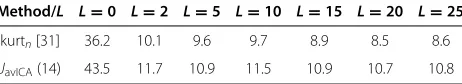
For L = 0, the mixture is instantaneous and separa-tion is possible with high SIR. But forL = 2 (filters with five taps) and for higher degree of mixing and de-mixing filters, the SIR decreases to about average 9 dB for audio-only method of [31] and 11 dB for the hybrid AV coherent and independent method proposed in Section 3.4.
6 Conclusion
In this paper, we proposed an improved AV associa-tion model using an MLP which exploits the dependency
between AV frames and is superior to the existing GMM AV model. The MLP model makes efficient use of its parameters relative to the GMM model. Hence, unlike the GMM model, it can capture temporal dynamics from a limited context of frames around the current frame to enhance the coherency measure. We also proposed a hybrid criterion which exploits AV coherency together with normalized kurtosis as an independence measure and, based on that, moved toward a time-domain convo-lutive AVSS method. Experimental results for comparison of the methods are presented in terms of the relevant sig-nal classification accuracy and also the separation output SIRs. Results, confirms the contribution of the proposed neural-based AV association model in enhancement of AV incoherency scores and hence in improvement of the separation SIRs compared to the existing GMM-based AVSS algorithm and the visually assisted ICA (JADE-AV) method. Also, results of the time-domain convolutive method, using hybrid AV criterion shows improvement compared to the reference audio-only method.
For visual parametrization part, we have used normal-ized PCA-projected (whitened) lip appearance features. PCA features do not need exact lip contour detection and hence require less computation compared to extraction of lip geometric (width and height) parameters. But it also has the drawback of being more sensitive to the speaker and segmentation of the lip region. The fitness of PCA features for AV modeling and AVSS task is justified by qualitative illustrations and numerical results. However, the proposed AVSS method is not coupled to the PCA visual features and it can be adopted with more robust and accurate visual features.
Although proposed model improves quality of AV mod-eling, but further enhancements is both required and predictable to make these methods applicable in more complex phonetic contexts and speaker-independent sit-uations. AV relation is both non-linear and stochastic.
Table 7 Average output SIRs in dB for 2×2 convolutive case
Method/L L=0 L=2 L=5 L=10 L=15 L=20 L=25
kurtn[31] 36.2 10.1 9.6 9.7 8.9 8.5 8.6
JavICA(14) 43.5 11.7 10.9 11.5 10.9 10.7 10.8
GMM benefits from its capability in probabilistic model-ing. But GMM fails to efficiently handle the non-linearity and temporal dependency. On the other hand, MLP seems to benefit from its relatively deep structure and effi-cient use of its parameters, but it does not truly consider stochastic property of AV relation. Further improvements may be gained by introducing a model which can effi-ciently handle both the non-linear and the stochastic relations of the two modalities as well as the temporal dependency. Also, it seems promising to consider more essential combinations of ICA- and AV coherency-based methods to jointly gain benefits of both informed and blind methods.
Finally, it is worth to mention that in this paper, we did not consider the inter-batch temporal dynamics of de-mixing vectors and separated signals. It is possible to adopt this temporal information for example using a Bayesian recursive filtering approach to improve the per-formance and speed of proposed methods. Also, it is pos-sible to adaptively determine the working batch size based on the amount of inter-batch variations of the de-mixing vectors.
Appendix
Here, we derive the gradient ∂Ye(k)
∂B which is required in
calculation of (11). The embedded acoustic vectorYe(k)
is composed from individual acoustic frames Y(k). So we first need to calculate the gradient ∂Y∂B(k) which is a Jacobian matrix of the sizeka×M. Starting from (17) and
(19), we have
n×M is Jacobian of PSD vector with
respect toB andis the element-wise operator which divides each column of the left matrix by the right vector. The Jacobian of PSD is also calculated as:
∂PSDBX(k)
Jacobian matrix of the PS vector with respect to Band
( i ∂PSi
BX(k)
∂B )1×Mis the sum of rows of the Jacobian matrix.
Finally, the Jacobian of PS is calculated as
∂PSBX(k) operators. Equations 22, 23 and 24 are derived for the cal-culation of Jacobian of a single frame. In our MATLAB implementation, we have derived more complex matrix forms which allows calculation of Jacobian of multiple acoustic frames (i.e. all frames in a batch) using effi-cient vectorized computing. Having Jacobian of individual acoustic framesY(k), we combine the theme to obtain the Jacobian of embedded acoustic vectorsYe(k). This is done
according to the definition of the embedding methodE.
Competing interests
The authors declare that they have no competing interests.
Acknowledgements
Authors would like to say thanks to the anonymous reviewers for their attention which solved some important presentation issues and also for providing improving suggestions.
Received: 7 July 2013 Accepted: 18 February 2014 Published: 5 April 2014
References
1. Sumby WH, Pollack I, Visual contribution to speech intelligibility in noise. J. Acoust. Soc. Am.26, 212–215 (1954)
2. Summerfield Q, Lipreading and audio-visual speech perception. Philos. Trans. R. Soc. Lond. B Biol. Sci.335(1273), 71–78 (1992)
3. KW Grant, P-F Seitz, The use of visible speech cues for improving auditory detection of spoken sentences. J. Acoust. Soc. Am.108, 1197 (2000) 4. H McGurk, J MacDonald, Hearing lips and seeing voices. Nature.
264(5588), 746–748 (1976)
5. J-L Schwartz, F Berthommier, C Savariaux, Seeing to hear better: evidence for early audio-visual interactions in speech identification. Cognition.
93(2), 69–78 (2004)
6. ED Petajan,Automatic lipreading to enhance speech recognition. (PhD thesis, University of Illinois, Illinois, 1984)
7. L Girin, J-L Schwartz, G Feng, Audio-visual enhancement of speech in noise. J. Acoust. Soc. Am.109(6), 3007–3020 (2001)
8. S Deligne, G Potamianos, C Neti, Audio-visual speech enhancement with AVCDCN (AudioVisual Code-book Dependent Cepstral Normalization), in
Proceedings of the ISCA International Conference on Spoken Language Processing (ICSLP’02)(ISCA, 2002), pp. 1449–1452
9. F Berthommier, Audiovisual speech enhancement based on the association between speech envelope and video features, inProceedings of the ISCA European Conference on Speech Communication and Technology (EUROSPEECH’03)(ISCA, 2002), pp. 1045–1048
11. B Rivet, L Girin, C Jutten, Visual voice activity detection as a help for speech source separation from convolutive mixtures. Speech Communication.49(7), 667–677 (2007)
12. D Sodoyer, J-L Schwartz, L Girin, J Klinkisch, C Jutten, Separation of audio-visual speech sources: a new approach exploiting the audio-visual coherence of speech stimuli. EURASIP J. Appl. Signal Process.2002(1), 1164–1173 (2002)
13. S Rajaram, AV Nefian, TS Huang, Bayesian separation of audio-visual speech sources, inProc. IEEE International Conference on Acoustics, Speech, and Signal Processing (ICASSP’04), vol. 5 (IEEE, 2004), pp. 657–661 14. D Sodoyer, L Girin, C Jutten, J-L Schwartz, Developing an audio-visual
speech source separation algorithm. Speech Commun.44(1), 113–125 (2004)
15. W Wang, D Cosker, Y Hicks, S Sanei, J Chambers, Video assisted speech source separation, inProc. IEEE International Conference on Acoustics, Speech, and Signal Processing (ICASSP’05), vol. 5 (IEEE, 2005), p. 425 16. B Rivet, L Girin, C Jutten, Mixing audiovisual speech processing and blind
source separation for the extraction of speech signals from convolutive mixtures. Audio, Speech, Lang. Process. IEEE Trans.15(1), 96–108 (2007) 17. C Sigg, B Fischer, B Ommer, V Roth, J Buhmann, Nonnegative CCA for
audiovisual source separation, inIEEE Workshop On Machine Learning for Signal Processing (MLSP’07)(IEEE, 2007), pp. 253–258
18. AL Casanovas, G Monaci, P Vandergheynst, R Gribonval, Blind audiovisual separation based on redundant representations, inIEEE International Conference on Acoustics, Speech, and Signal Processing (ICASSP’08)(IEEE, 2008), pp. 1841–1844
19. G Monaci, F Sommer, P Vandergheynst, Learning sparse generative models of audiovisual signals, inEURASIP European Signal Processing Conference (EUSIPCO ’08), vol. 4 (EURASIP, 2008)
20. G Monaci, P Vandergheynst, FT Sommer, Learning bimodal structure in audio–visual data. Neural Netw. IEEE Trans.20(12), 1898–1910 (2009) 21. AL Casanovas, G Monaci, P Vandergheynst, R Gribonval, Blind audiovisual
source separation based on sparse redundant representations. Multimedia, IEEE Trans.12(5), 358–371 (2010)
22. Y Liang, SM Naqvi, JA Chambers, Audio video based fast fixed-point independent vector analysis for multisource separation in a room environment. EURASIP J. Adv. Signal Process.2012(1), 1–16 (2012) 23. Q Liu, W Wang, PJ Jackson, M Barnard, J Kittler, JA Chambers, Source
separation of convolutive and noisy mixtures using audio-visual dictionary learning and probabilistic time-frequency masking. IEEE Trans. Signal Process.61(22) (2013)
24. MS Khan, SM Naqvi, A Rehman, W Wang, JA Chambers, Video-aided model-based source separation in real reverberant rooms. IEEE Trans. Audio Speech Lang. Process.21(9), 1900–1912 (2013)
25. AJ Bell, TJ Sejnowski, An information-maximization approach to blind separation and blind deconvolution. Neural Computat.7(6), 1129–1159 (1995)
26. A Hyvärinen, E Oja, A fast fixed-point algorithm for independent component analysis. Neural Comput.9(7), 1483–1492 (1997) 27. J-F Cardoso, High-order contrasts for independent component analysis.
Neural Comput.11(1), 157–192 (1999)
28. J Jeffers, M Barley,Speechreading (lipreading). (Charles C. Thomas Publisher, Springfield, Illinois, 1971)
29. L Cappelletta, N Harte, Phoneme-to-viseme mapping for visual speech recognition, inProceedings of the International Conference on Pattern Recognition Applications and Methods (ICPRAM 2012)(IEEE, 2012), pp. 322–329
30. N Delfosse, P Loubaton, Adaptive blind separation of independent sources: a deflation approach. Signal Process.45(1), 59–83 (1995) 31. JK Tugnait, Identification and deconvolution of multichannel linear
non-Gaussian, processes using higher order statistics and inverse filter criteria. Signal Process. IEEE Trans.45(3), 658–672 (1997)
32. V Zarzoso, P Comon, Robust independent component analysis by iterative maximization of the kurtosis contrast with algebraic optimal step size. Neural Netw. IEEE Trans.21(2), 248–261 (2010)
33. S Gazor, W Zhang, Speech probability distribution. Signal Process. Lett. IEEE.10(7), 204–207 (2003)
34. I Tashev, A Acero, Statistical modeling of the speech signal, inProc. Intl. Workshop on Acoustic, Echo, and Noise Control (IWAENC 2010)(IEEE, 2010) 35. J Thomas, Y Deville, S Hosseini, Time-domain fast fixed-point algorithms
for convolutive ICA. Signal Process. Lett. IEEE.13(4), 228–231 (2006)
36. F Moayedi, A Kazemi, Z Azimifar, Hidden Markov model-unscented Kalman filter contour tracking: a multi-cue and multi-resolution approach, inIranian Conference on Machine Vision and Image Processing (MVIP 2010)
(IEEE, Piscataway, 2010), pp. 1–6
37. AP Dempster, NM Laird, DB Rubin, Maximum likelihood from incomplete data via the EM algorithm. J. R. Stat. Soc. Series B (Methodological).39(1), 1–38 (1977)
38. MT Hagan, M Menhaj, Training feed-forward networks with the Marquardt algorithm. IEEE Trans. Neural Netw.5(6), 989–993 (1994) 39. E Vincent, R Gribonval, C Févotte, Performance measurement in blind
audio source separation. Audio, Speech, Lang. Process. IEEE Trans.14(4), 1462–1469 (2006)
doi:10.1186/1687-6180-2014-47
Cite this article as:Kazemiet al.:Audio visual speech source separation via improved context dependent association model.EURASIP Journal on Advances in Signal Processing20142014:47.
Submit your manuscript to a
journal and benefi t from:
7Convenient online submission 7Rigorous peer review
7Immediate publication on acceptance 7Open access: articles freely available online 7High visibility within the fi eld
7Retaining the copyright to your article