P R O C E E D I N G S
Open Access
Genomic breeding value prediction using three
Bayesian methods and application to reduced
density marker panels
Matthew A Cleveland
1*, Selma Forni
1, Nader Deeb
1, Christian Maltecca
2From
13th European workshop on QTL mapping and marker assisted selection
Wageningen, The Netherlands. 20-21 April 2009
Abstract
Background:Bayesian approaches for predicting genomic breeding values (GEBV) have been proposed that allow for different variances for individual markers resulting in a shrinkage procedure that uses prior information to coerce negligible effects towards zero. These approaches have generally assumed application to high-density genotype data on all individuals, which may not be the case in practice. In this study, three approaches were compared for their predictive power in computing GEBV when training at high SNP marker density and predicting at high or low densities: the well- knownBayes-A,a generalization ofBayes-Awhere scale and degrees of freedom are estimated from the data (Student-t) and a Bayesian implementation of theLasso method. Twelve scenarios were evaluated for predicting GEBV using low-density marker subsets, including selection of SNP based on genome spacing or size of additive effect and the inclusion of unknown genotype information in the form of genotype probabilities from pedigree and genotyped ancestors.
Results:The GEBV accuracy (calculated as correlation between GEBV and traditional breeding values) was highest forLasso,followed byStudent-tand then Bayes-A.When comparing GEBV to true breeding values,Student-twas most accurate, though differences were small. In general the shrinkage applied by theLasso approach was less conservative thanBayes-AorStudent-t, indicating thatLasso may be more sensitive to QTL with small effects. In the reduced-density marker subsets the ranking of the methods was generally consistent. Overall, low-density, evenly-spaced SNPs did a poor job of predicting GEBV, but SNPs selected based on additive effect size yielded accuracies similar to those at high density, even when coverage was low. The inclusion of genotype probabilities to the evenly-spaced subsets showed promising increases in accuracy and may be more useful in cases where many QTL of small effect are expected.
Conclusions:In this dataset theStudent-tapproach slightly outperformed the other methods when predicting GEBV at both high and low density, but theLassomethod may have particular advantages in situations where many small QTL are expected. When markers were selected at low density based on genome spacing, the inclusion of genotype probabilities increased GEBV accuracy which would allow a single low- density marker panel to be used across traits.
* Correspondence: [email protected]
1Genus plc., 100 Bluegrass Commons Blvd., Suite 2200, Hendersonville, TN,
37075, USA
Background
A number of approaches have recently been proposed for the prediction of genomic breeding values for high-den-sity single nucleotide polymorphism (SNP) panels. Meth-ods commonly used fall into two categories,BLUPand Bayesian approaches. In aBLUPframework SNP effects are sampled from a normal distribution and the variance is assumed constant across SNPs [1]. In a Bayesian approach prior knowledge about the distribution of SNP effects is assumed, generally that many SNPs are likely to have small individual effects and only a few will have large effects [2], allowing for different variances for indi-vidual SNPs. This assumption results in a shrinkage pro-cedure in which the prior information is used to coerce negligible effects toward zero. Different derivations of this shrinkage approach have been proposed, including Bayes-A[1]. In this method a scaled inverse-c2prior is assigned to SNP variances. Scale and degrees of freedom of the distribution are in this case set as hyperparameters and samples of the posterior distribution are obtained through MCMC methods. A generalization in which the hyperparameters regulating the shrinkage are treated as unknown parameters and estimated from the data leads to the well knownStudent-tmodel [3] where the amount of shrinkage is controlled by the data. Alternative shrink-age approaches have also been recently proposed. A par-ticularly appealing method is the least absolute shrinkage and selection operator (Lasso) [4]. In its Bayesian inter-pretationLassoestimates can be seen as posterior mode estimates when the regression parameters have indepen-dent and iindepen-dentical Laplace priors. Yi and Xu [5] recently comparedLassoandStudent-tmodels for QTL mapping. Prediction of genomic breeding values can be seen as a generalization of the same problem. It has been reported [6,7] that Bayesian methods give higher genomic breed-ing value accuracies thanBLUPmethods. There are few published results, though, on the performance of differ-ent shrinkage methods for genomic breeding value pre-diction. These approaches were initially developed assuming dense genome- wide SNP coverage. This may not be the case in practice as it is often cost prohibitive to genotype all animals at high density and it may be desired to predict genomic breeding values using low density panels.
This study investigated the predictive performance of different Bayesian hierarchical approaches,Bayes-A, Stu-dent-tandLasso,when training and predicting genomic breeding values at high density and when predicting at lower densities.
Methods
The dataset used for analysis was simulated as part of the 13thQTL-MAS Workshop, see [8] for details. The
data consisted of 5 sires, 20 dams and 2000 offspring, of which 1000 had phenotypes. The 1000 phenotyped off-spring made up the training set, while the 1000 un-phe-notyped offspring comprised the prediction set for calculation of genomic breeding values (GEBV). All indi-viduals were genotyped for 453 SNP markers, approxi-mately equally-spaced across five chromosomes of length one Morgan each.
Prediction of phenotypes and breeding values
The simulated dataset included phenotypes for five traits representing measures of yield at five different time points (t0, t132, t265, t397 and t530). A sixth phenotype was predicted to represent yield at a time point beyond the simulated data, time point 600 (t600). A number of non-linear models were tested to predict t600 [9-12], and the Gompertz model [12] was found to best fit the data according to AIC [13] and BIC [14] measures. Least squares estimates of growth curve parameters were obtained for each individual using the procedure
“NLIN” from SAS [15]. Individual growth curve para-meters could then be used to calculate individual phe-notypic predictions for any time point until maturity, including t600. Traditional breeding values were esti-mated using a single trait linear model for each of the time points. We report the results for t530 and t600.
Description of models
The data were analyzed using three different approaches, considering additive genetic effects only. The general structure of the models in matrix form was:
y 1 X + e
where y is the vector of phenotypic effects, µ is the overall mean,bis the vector of additive effects for each marker,Xis a matrix of genotypes expressed as number of copies of an arbitrary allele (0,1,2) for each SNP and
eis a vector of residuals assumed N(0,e2). All models
were considered as two level hierarchical models. A flat (1) and a non informative (1/e2) prior were assigned to
µ and e2, respectively. The remaining prior structure
was:
j~N( ,0gi2)
for the jthSNP,
gi2 ~Exp(gi2| /2 j2)
for theLassoapproach and
for the Bayes-AandStudent-tapproaches. Degrees of freedomvand scale parameters2for Bayes-Awere con-sidered hyperparameters and were assigned values as in [1]. The Student-tmodel treated vand s2 as unknown and assigned a uniform density of 1/vfor the interval (0,1] and a uniform distribution ofsfor the range (0,A], with A being a large number [5]. The lparameter in theLassoapproach was assigned a gamma prior distri-butionGamma(a,b). Values ofaandb were set at 0.05 and 1.0, respectively, so that prior of lwas essentially uniform over a wide range of values. The Lasso approach differs slightly from that of Park and Casella [16] and de los Campos [17], which is guaranteed to provide unimodal posteriors of effects. A Gibbs sam-pling algorithm was implemented to obtain samples from the joint posterior distribution. Steps of the algo-rithm are outlined below (for details on conditional pos-terior distribution see [5]):
1) Sample µ from N(µ|y,b,e2)
2) Sample bj from N(b | y, µ,e2,gi2), where the updates in this case are obtained though Gauss-Sei-del with residual update [18]
3) Samplee2from Inv−c
The Gibbs sampling algorithm for all three methods was implemented in R [19]. For each analysis a single chain of 15000 iterations was run with a burn-in period of 5500 iterations. Samples were stored every 30 iterations. Con-vergence of each chain was assessed both by visual inspec-tion of the trace and the use of estimates of effective sample size for the variances obtained through the R coda package [20]. Inferences on the parameters were made on the average of the posterior samples after burn-in.
Genomic breeding values were calculated for all indi-viduals in the prediction set, for t530 and t600 by:
GEBV Xm m
whereXm is a matrix of genotypes expressed as (0,1,2)
andbmis a vector of posterior mean effects for a
parti-cular method, formSNPs. A cross validation procedure was also used where phenotyped individuals were ran-domly split into training and prediction sets (90%
training; 10% prediction) 10 times to assess the stability of the genomic predictions for t530 and t600.
Low-density marker subsets
Subsets of the prediction dataset were created to simulate the situation where training can be done at high density, but prediction of GEBV occurs with a lower density panel. In this case the full training set, including 1000 individuals and 453 SNPs, was used to estimate the SNP effects, but GEBV were calculated using either a smaller subset of SNPs or a combination of genotypes for a small subset and genotype probabilities for the remaining mar-kers (see Table 1). Genomic breeding values were calcu-lated for 12 subset scenarios without retraining on the subset markers, using each of the three methods, for t530 and t600. One-half of the data subsets included only a small number of markers spaced evenly across the gen-ome (m=19, 38 or 76) or a small number of markers with the largest absolute effects in each of the respective methods and traits (m=19, 38 or 76). These SNP num-bers were chosen to approximate the low-density panels that could potentially be used in livestock species (e.g., 384 in pigs or cattle). These GEBV calculations used effects only for these (m) markers from the training set. For each of the subsets above another subset was tested including genotype probabilities for all of the remaining markers in calculation of the GEBV. Each of these sub-sets contained all markers, and thus these GEBV calcula-tions used all high-density SNP effects from training, but only a small subset of markers had actual genotypes (m=19, 38 or 76). The genotype probabilities were calcu-lated through marker and pedigree information from the full dataset, for all individuals in the prediction set, using segregation analysis for single markers following Kerr and Kinghorn [21].
Genomic breeding values were calculated for the mar-ker subsets as above by:
GEBV Xm m
In this case, the individual element (i) of Xmis calcu-lated as:
Xmjj (1) P 2 (2)P
whereP(1) andP(2)are the probabilities of individual (i) having the heterozygous and homozygous (coded as 2) genotypes, respectively, for each marker (j). When the actual genotype is known the matrix element is simply coded as before (0,1,2). This approach is related to the genetic predictor approach of Boeret al.[22].
Results
correlation between the GEBV and estimated breeding values (EBV) calculated using the traditional animal model, for all animals in the prediction set (Table 2). The three approaches performed similarly with Lasso yielding the highest accuracy, followed byStudent-tand thenBayes-A.The difference between the top and bot-tom accuracies was about 6%. Results were consistent across t530 and t600. Coefficients of regression of EBV on GEBV were nearly identical for all methods, across traits, indicating little or no difference in bias exists. Cross- validation using ten replicates from the training dataset found differences between the three approaches consistent with Table 2 (results not shown).
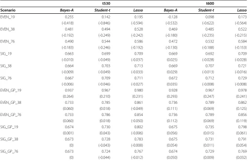
Correlations of GEBV for each low-density SNP sce-nario (Table 1) and EBV (including the change in corre-lation compared to GEBV calculated using all markers in the prediction set) are shown in Table 3, to represent the change in GEBV accuracy using the low-density approach. In all cases the accuracy increased (or stayed the same) when increasing the number of markers with genotypes in the subset. The scenarios where evenly-spaced markers were included had lower accuracies than the same density subset where SNPs with the lar-gest effects were included. There appears to be an advantage to using genotype probabilities with evenly-spaced markers, particularly in the case with few marker genotypes (EVEN_19) with accuracies approaching 1. The differences between the three models were similar to those found when using all markers in the prediction set (Table 2), but the reductions in accuracy using Bayes-A were the smallest in nearly all cases. When using SNPs with the largest effects (with and without genotype probabilities), the GEBV calculated using Bayes-A were essentially the same as GEBV calculated using all markers. There was little loss in accuracy by reducing the marker set from 453 to 19 (with the largest
effects) for all methods. The reductions in accuracy resulting fromLassomarker effects were generally simi-lar to the other methods for all low-density subsets and the accuracy was still superior toBayes-AandStudent-t in all cases. In a number of the scenarios the accuracy actually increased from high-density to low-density. Many of the increases were small and thus the accura-cies were practically unchanged, but large increases in accuracy were observed for subsets with evenly-spaced SNPs and genotype probabilities, particularly EVEN_GP_19.
Discussion
The three methods applied to the simulated data per-formed similarly (Table 2), where the accuracy using Lasso was the highest, Student-t was next and then Bayes-A, though differences were small. The accuracy in this case was the correlation between GEBV and EBV, which is the limit of information currently available, and thus the reported accuracies will likely change when true breeding values are available. In general, methods based on inverse -c2 priors (Bayes-A and Student-t) appear to be more conservative in the shrinkage than Lasso, even when the scale and degrees of freedom
Table 1 Number of SNPs included in the calculation of genomic breeding values in each low-density scenario
Scenario Evenly-spaceda Largest effectsb Genotype probabilitiesc Total
EVEN_19 19 19
EVEN_38 38 38
EVEN_76 76 76
SIG_19 19 19
SIG_38 38 38
SIG_76 76 76
EVEN_GP_19 19 434 453
EVEN_GP_38 38 415 453
EVEN_GP_76 76 377 453
SIG_GP_19 19 434 453
SIG_GP_38 38 415 453
SIG_GP_76 76 377 453
a
Selected by taking themth
SNPs from ordered list and thus SNP were approximately evenly-spaced b
Selected by taking the topmSNPs from a list ordered by absolute effect, for each analysis method c
Genotype probabilities were used in place of actual genotypes for all SNPs that don’t fall into one of the other categories, within a scenario
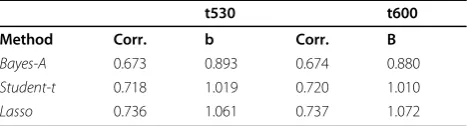
Table 2 Correlations between genomic breeding values and breeding values from a traditional animal model for animals in the prediction set (without phenotypes) and coefficients of regression of traditional on genomic breeding values, for t530 and t600.
t530 t600
Method Corr. b Corr. B
Bayes-A 0.673 0.893 0.674 0.880
Student-t 0.718 1.019 0.720 1.010
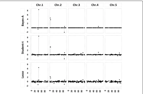
parameters are estimated from the data (Figure 1). These parameters estimated byStudent-tand Lassoall converged to the same values (within method) across the cross-validation replicates, indicating that this data-set included sufficient information for estimation. The marker effects shown in Figure 1 suggest thatLassomay be more sensitive to QTL with small effects than Stu-dent-t,which in turn is more sensitive thanBayes-A.
The use of low-density SNP subsets is based on the concept of Habier et al.[23] where SNP effects are esti-mated from a training dataset using high-density SNP genotypes, but GEBV are then calculated for individuals genotyped for only a small subset of the SNPs. These subsets may be chosen by selecting markers for even genome coverage or based on effect size for a certain trait, where un-genotyped SNPs may be filled in to approximate high-density coverage. The current analysis found that evenly-spaced SNPs alone did a poor job of predicting GEBV (Table 3). By chance this approach could produce high GEBV accuracies if selected SNPs happened to be in linkage disequilibrium (LD) with large QTL for a particular trait, but in general it would be expected that many QTL would not be represented
by the low-density panel. In the current dataset average LD was low (results not shown) which explains the poorer performance of the evenly-spaced, low-density subset compared to other approaches. Selecting only SNPs with large effects in each of the three methods yielded GEBV that were nearly as accurate as when using all markers, in all cases. This result is likely speci-fic to the case where few QTL of large or moderate effect are expected and thus few markers will account for most of the variance, which is presumed in this data-set based on Figure 1. In fact, the correlation between GEBV and EBV for t600 in the prediction set was 0.603 using the three SNPs with largest effects in Bayes-A, only a 7% reduction in accuracy.
The scenarios using genotype probabilities performed well and in most cases showed a small or no reduction in accuracy, compared to using the full marker set. Due to the population structure (full and half-sib families) and completeness of parental genotypes it is expected that the genotype probabilities are a good representation of the true genotypes in this case. In a situation where there are fewer ties between individuals the advantage of using genotype probabilities (in place of actual genotypes) is
Table 3 Correlations between genomic breeding values and breeding values from different low SNP-density
approaches (and change in correlation compared to original full marker model), where all SNP effects are estimated in the same high SNP-density training set, for t530 and t600.
t530 t600
Scenario Bayes-A Student-t Lasso Bayes-A Student-t Lasso
EVEN_19 0.255 0.142 0.195 -0.128 0.098 0.173
(-0.418) (-0.846) (-0.594) (-0.532) (-0.622) (-0.564)
EVEN_38 0.481 0.494 0.528 0.469 0.485 0.522
(-0.192) (-0.249) (-0.242) (-0.180) (-0.235) (-0.215)
EVEN_76 0.490 0.544 0.586 0.472 0.532 0.584
(-0.183) (-0.246) (-0.192) (-0.130) (-0.188) (-0.153)
SIG_19 0.663 0.699 0.709 0.669 0.692 0.709
(-0.010) (-0.049) (-0.037) (0.025) (-0.028) (-0.028)
SIG_38 0.664 0.703 0.713 0.669 0.707 0.721
(-0.009) (-0.049) (-0.033) (0.029) (-0.013) (-0.016)
SIG_76 0.667 0.709 0.711 0.672 0.712 0.729
(-0.006) (-0.046) (-0.027) (0.035) (-0.008) (-0.008)
EVEN_GP_19 0.937 0.967 0.980 0.928 0.967 0.978
(0.264) (0.210) (0.231) (0.293) (0.247) (0.241)
EVEN_GP_38 0.733 0.785 0.861 0.736 0.789 0.862
(0.060) (0.018) (-0.049) (0.111) (0.069) (0.125)
EVEN_GP_76 0.733 0.786 0.854 0.736 0.789 0.856
(0.060) (0.018) (-0.050) (0.112) (0.069) (0.119)
SIG_GP_19 0.674 0.730 0.802 0.675 0.735 0.798
(0.001) (0.043) (-0.006) (0.056) (0.015) (0.061)
SIG_GP_38 0.673 0.728 0.783 0.675 0.731 0.791
(0) (-0.043) (-0.008) (0.054) (0.011) (0.054)
SIG_GP_76 0.673 0.724 0.767 0.674 0.729 0.769
likely to be lower than what was found in this study. A number of the scenarios even showed large increases in accuracy to unrealistic levels (e.g., EVEN_GP_19, Table 3). Paradoxically, the evenly-spaced scenarios outper-formed the largest SNP effects scenarios, where the best performance came from the smallest number of SNPs. This result can be attributed to calculating accuracy based on the EBV. With fewer markers and less informa-tion (based on even spacing) the GEBV calculated in EVEN_GP_19 are nearly identical within family and are implicitly based on family relationships, through SNP allele sharing, and thus the GEBV are approximations of the EBV rather than the true breeding value. Using the EBV as a proxy for the true breeding value appears to be a poor choice in this case. Addition of true breeding values should make this a fairer comparison.
Epilogue
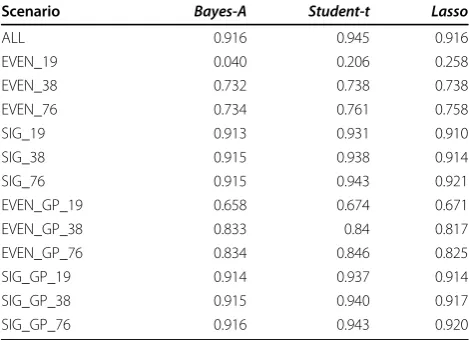
The availability of true breeding values (TBV) allowed for an improved evaluation of the effectiveness of the three analysis methods on alternative marker sets (Table 4). As expected, the correlations improved when com-paring GEBV to TBV, instead of EBV. The accuracy of each of the methods was high when using all markers, with Student-tyielding the highest value (0.945). The
of SNPs with large effects would be enough to obtain high accuracy GEBV while greatly reducing genotyping requirements. The results from using genotype probabil-ities are promising but are likely best applied in situa-tions where many small QTL are expected.
Conclusions
For this simulated dataset theLassomethod slightly out-performed Bayes-A and Student-t when considering accuracy as the correlation between GEBV and EBV, but Student-tperformed the best when comparing GEBV to TBV. Bayes-Aand Student-tappeared to be more con-servative in shrinkage of SNP effects indicating that Lasso may be more sensitive to small QTL and thus may perform better than other methods for traits where large or moderate QTL are not expected. In the analysis of reduced marker density few SNPs were needed to maintain levels of accuracy similar to the high-density SNP set when SNPs with large effect were selected. When markers were selected based on spacing, the use of genotype probabilities in place of known genotypes increased the accuracy of the GEBV, which would allow a single low-density panel to be used across traits.
Acknowledgement
This article has been published as part of BMC Proceedings Volume 4 Supplement 1, 2009: Proceedings of 13th European workshop on QTL mapping and marker assisted selection.
The full contents of the supplement are available online at http://www.biomedcentral.com/1753-6561/4?issue=S1.
Author details
1Genus plc., 100 Bluegrass Commons Blvd., Suite 2200, Hendersonville, TN,
37075, USA.2North Carolina State University, Department of Animal Science, Raleigh, NC, 27695-7627, USA.
Authors’contributions
MAC performed analyses, participated in study design and drafted the manuscript. SF performed analyses and participated in study design. ND participated in study design and helped to interpret results. CM developed the methods for effect estimation, performed analyses, participated in study design and helped draft the manuscript. All authors read and approved the final manuscript.
Competing interests
The authors declare that they have no competing interests.
Published: 31 March 2010
References
1. Meuwissen THE, Hayes BJ, Goddard ME:Prediction of total genetic value using genome-wide dense marker maps.Genet2001,157:1819-1829. 2. Hayes BJ, Goddard ME:The distribution of the effects of genes affecting
quantitative traits in livestock. Genet. Sel. Evol.2001,33:209-229. 3. Andrews DF, Mallows CL:Scale mixtures of normal distributions.J Royal
Stat Soc B-Methodological1974,36:99-102.
4. Tibshirani R:Regression shrinkage and selection via the lasso.J Royal Stat Soc B1996,58:267-288.
5. Yi N, Xu S:Bayesian LASSO for quantitative trait loci mapping.Genet
2008,179:1045-1055.
6. VanRaden PM:Efficient methods to compute genomic predictions.J Dairy Sci2008,91:4414-4423.
7. VanRaden PM, Van Tassell CP, Wiggans GR, Sonstegard TS, Schnabel RD, Taylor JF, Schenkel FS:Invited review: Reliability of genomic predictions for North American Holstein bull.J Dairy Sci2009,92:16-24.
8. Coster A, Bastiaansen J, Calus M, Maliepaard C, Bink M:QTLMAS 2009: Simulated dataset.BMCProc2010,4(Suppl 1):S3.
9. Brody S:Bioenergetics and growth.Reinhold Publishing Corp. 1945. 10. Von Bertalanffy L:Quantitative laws in metabolism and growth.The
Quarterly Review of Biology1957,32:217-230.
11. Nelder JA:The fitting of a generalization of the logistic curve.Biometrics
1961,17:89-110.
12. Laird AK:Dynamics of relative growth.Growth1965,29:249-263. 13. Akaike H:A new look at the statistical model identification.IEEE Trans
Autom Control1974,19:716-723.
14. Schwarz G:Estimating the dimension of a model.Annals of Stat1978, 6(8):461-464.
15. SAS Institute Inc:SAS 9.2 Help and Documentation.2009.
16. Park T, Casella G:The Bayesian Lasso.JAmer Stat Soc2008,103:681-686. 17. de los Campos G, Naya H, Gianola D, Crossa J, Legarra A, Manfredi E,
Weigel K, Cotes JM:Predicting quantitative traits with regression models for dense molecular markers and pedigree.Genet2009,182:375-385. 18. Legarra A, Misztal I:Technical Note: Computing strategies in
genome-wide selection.J Dairy Sci2008,91:360-366.
19. R Development Core Team:R: A language and environment for statisitcal computing.2008.
20. Plummer M, Best N, Cowles K, Vines K:CODE: Convergence diagnosis and output analysis for MCMC.R News2006,6:7-11.
21. Kerr RJ, Kinghorn BP:An efficient algorithm for segregation analysis in large populations.JAnim Breed Genet1996,113:457-469.
22. Boer MP, Wright D, Feng L, Podlich DW, Luo L, Cooper M, van Eeuwijk FA: A mixed-model quantitative trait loci (QTL) analysis for multiple-environment trial data using multiple-environmental covariables for QTL-by-environment interactions, with an example in Maize.Genet2007, 177:1801-1813.
23. Habier D, Fernando RL, Dekkers JCM:Genomic selection using low-density marker panels.Genet2009,182:343-353.
doi:10.1186/1753-6561-4-S1-S6
Cite this article as:Clevelandet al.:Genomic breeding value prediction using three Bayesian methods and application to reduced density marker panels.BMC Proceedings20104(Suppl 1):S6.