R E S E A R C H
Open Access
Sub-sampling-based 2D localization of an
impulsive acoustic source in reverberant
environments
Muhammad Omer
1*, Ahmed A Quadeer
1, Mohammad S Sharawi
1and Tareq Y Al-Naffouri
1,2Abstract
This paper presents a robust method for two-dimensional (2D) impulsive acoustic source localization in a room environment using low sampling rates. The proposed method finds the time delay from the room impulse response (RIR) which makes it robust against room reverberations. We consider the RIR as a sparse phenomenon and apply a recently proposed sparse signal reconstruction technique called orthogonal clustering (OC) for its estimation from the sub-sampled received signal. The arrival time of the direct path signal at a pair of microphones is identified from the estimated RIR, and their difference yields the desired time delay estimate (TDE). Low sampling rates reduces the hardware and computational complexity and decreases the communication between the microphones and the centralized location. Simulation and experimental results of an actual hardware setup are presented to demonstrate the performance of the proposed technique.
Keywords: Impulsive source localization; Room impulse response (RIR); Orthogonal clustering (OC); Sub-sampling
1 Introduction
Time delay estimation (TDE)-based localization methods are suitable for wideband source signals, and many algo-rithms [1-5] have been proposed for TDE-based localiza-tion. Such systems can be divided into two categories. The first one assumes the presence of the sound source in the far field of the microphone array. The sound wavefronts arriving at the microphones are planar, and TDE from a pair of microphones can be used to find the direction of arrival (DOA) of the signal [6]. Several DOA estimates from spatially separated microphone arrays are used to find the source location.
Another TDE-based method called the time difference of arrival (TDOA), assumes the presence of the sound source in the near field of the microphones [7-10]. The TDE from a pair of microphones is converted into range difference from which the range difference equation is formed. Multiple range difference measurements lead to multiple equations which can be solved for the unknown source position [11,12]. With an increased number of
*Correspondence: [email protected]
1Electrical Engineering Department, King Fahd University of Petroleum & Minerals, Dhahran 31261, Saudi Arabia
Full list of author information is available at the end of the article
microphones, the ambiguity in the source location can be resolved by the least squares solution for the multiple range difference equations.
An accurate TDE is vital for both relative angles (DOA) and range-based (TDOA) localization schemes. The most basic TDE methods are the cross-correlation (CC)-based ones [2]. The CC method assumes an ideal sound prop-agation model which makes it suitable for low-noise and reverberant-free outdoor environments. The improved version of the CC method is the generalized cross-correlation (GCC) method [13]. The GCC is a family of algorithms which applies various weight functions to the received signal (pre-filters) in order to improve the TDE performance in noisy environment. Despite much improvement in GCC over the CC method, GCC method suffers from performance degradation in dense reverber-ant environments [14]. The performance of GCC method under real reverberant conditions has been analyzed in [15], and several improvements have been proposed. The fundamental problem with CC and GCC methods is their assumption that the microphones receive only the direct path signal. In [16], an adaptive eigenvalue decomposi-tion (AED) algorithm has been proposed that assumes more realistic sound propagation models for TDE in a
room reverberant environment. It first estimates the room impulse response (RIR) between the source and the pair of microphones. The TDE estimate is determined by identi-fying the direct paths from the two RIR. The AED algo-rithm for RIR estimation is a computationally complex algorithm with complexity ofO(N2). For AED to converge to the true RIR, it requires continuous snapshots of the source signal. This makes AED-based TDE unsuitable for the sources which are impulsive in nature.
In addition, these TDE techniques suffer from a time resolution problem at low sampling frequencies. The effect of under-sampling on the performance of these algorithms is discussed in [17]. The high sampling fre-quency requirement makes the localization process not only computationally intensive but also demands sophis-ticated hardware. In [5], the authors provide a brief overview, performance comparison, and problems associ-ated with widely used TDE methods. For example, the CC method requires the acquired data to be sent to a central processing unit for TDE. This puts stress on the commu-nication link as at high sampling rates, a large amount of data has to be communicated from the sensor to the central processing unit.
1.1 Motivation and main objectives
The drawbacks of the available TDE techniques motivated us in this work to find a better solution for TDE. In this work, a recently developed sparse signal reconstruction algorithm called orthogonal clustering (OC) is applied for the TDE problem [18]. This algorithm has already been successfully implemented for impulsive noise estimation and cancellation in digital subscriber lines (DSL) [19]. The objectives of this work are as follows:
1. To tune the algorithm in [18] and apply it to enhance the robustness of an indoor acoustic source
localization system against dense room reverberations.
2. To work at extremely low sampling rates to relax the computational and hardware complexity.
3. To build a hardware setup and investigate the algorithm performance in a real reverberant environment using actual measurements.
4. To benchmark the algorithm performance in terms of localization accuracy and computation time against a CC-based method.
The proposed method finds the time delays from the estimated RIR which makes it robust against room rever-berations. The RIR can be considered to be a sparse phenomenon when a finite number of non-zero and tem-porally separated impulses (corresponding to the reflected signal components) are observed for a relatively large time interval. This sparsity assumption is utilized to estimate
the RIR using OC algorithm [20]. The OC method recon-structs the sparse signals from the sub-sampled data which reduces the hardware and computational complex-ity. The arrival time of the direct path signal at a pair of microphones is identified from the estimated RIR, and their difference yields the desired TDE. These estimates are then used for the localization of the impulsive acoustic source using TDOA.
1.2 Paper organization
This paper is organized as follows: In Section 2, the signal model for RIR estimation is presented. A brief overview of sparse signal reconstruction methods and their appli-cations in different fields is given in Section 3. The details of the OC algorithm are presented in Section 4, followed by the description of the proposed TDE method based on OC in Section 5. The numerical and experimental results of the TDE-based source localization utilizing the OC algorithm are presented in Section 6. A discussion on the results is given in Section 7 and the concluding remarks in Section 8.
2 Signal model for sparse signal estimation
TDE is a challenging task in reverberant environments. The room environment between the source-microphone pair separated by some distance can be modeled as a finite impulse response (FIR) filter with a finite response termed as the RIR. The channel taps of this filter represent the multi-path components in the received signal. From the RIR, the direct line of sight (DLOS) signal can be identi-fied from the reflected ones. Thus, the problem of TDE is equivalent to an accurate RIR estimation at a pair of microphones and identification of the DLOS components [5,21].
The signal received at the microphone due to a known excitation signals(t)can be described by a multi-path sig-nal propagation model. The source sigsig-nals(t)is assumed to be of impulsive nature with a few non-zero values for a short time durationT. The received signaly(t)is given by
y(t)=
L−1
l=0
αls(t−τl)+n(t), (1)
where L is the number of paths capturing most of the
multi-path energy,αlandτlare the scaling magnitude fac-tor and the time shift of path l, respectively, while n(t) is the additive white Gaussian noise (AWGN). The dis-crete time representation of the model given in (1) can be compactly written as
y=α+n, (2)
with zero-mean and covariance matrixCn=σn2I. TheN×
Nmatrixis the sensing matrix whose columns consist
ofNdiscretized and delayed versions of the source signal s(t), i.e.,
S represent the time resolution withFSbeing
the sampling frequency. The sampling frequency FS is
assumed to satisfy the Nyquist criteria and thus <<T. The sub-sampled received signalris given as
r=α+ ´n, (4)
wherer∈RMis the sub-sampled received signal andn´ ∈
RMis the AWGN of the same mean and covariance matrix
as ofn. The matrix(of sizeM×N) is a uniformly sub-sampled version of the sensing matrixwhereM<<N and the sub-sampling ratio1 is N
M =
FS
FM. AsM << N, (4) is an under-determined system of equations and thus is ill-posed.
The room impulse response α can be assumed as a
sparse signal when the lengthNof the impulse response vector is much greater than the number of reflected signal componentsL, i.e.,N >>L. The sparsity information of the RIR helps in its reconstruction from a small number of measurements obtained from subsampling the received signal using compressed sensing theory as discussed in the next section.
3 Sparse signal estimation techniques
Sparse signal reconstruction has largely been facilitated since the advent of compressed sensing (CS). As the name suggests, the scheme acquires a signal at compressed sam-pling rates by randomly projecting it onto a subspace much smaller than the signal dimension. Most of the naturally occurring signals are sparse in some domain, and thus, CS techniques are able to reconstruct a sig-nal sampled at sub-Nyquist rates. This has successfully been implemented in peak-to-average power reduction in orthogonal frequency domain multiplexing (OFDM), image processing [22], impulse noise estimation and can-cellation in power-line communication and DSL [19], magnetic resonance imaging (MRI) [23], channel esti-mation in communication systems [24], ultra-wideband (UWB) channel estimation [25], DOA estimation [26], and radar design [27].
The number of measurementsMare less than the
num-ber of the unknownsN in (4) which renders the system
of equations as under-determined. This implies that an infinite number of α’s satisfy (4). This makes the prob-lem ill-posed, but it can be solved using the sparse nature ofα. The optimal solution in this cases is to solve an0
minimization problem. The 0minimization problem is
NP-hard and thus is not practical [28].
An alternate approach called convex relaxation solves
a relaxed 1 minimization problem by linear
program-ming instead of 0 minimization with a penalty on the
number of observations. Given that the sensing matrix
obeys certain properties, 1 minimization approach
gives accurate estimates of the sparse signal [29,30]. These methods do well in recovering the sparse signals from under-determined system, but at the same time, they suf-fer from a number of drawbacks. Some of these drawbacks are listed below:
1. Convex relaxation approaches are relatively computationally complex.
2. The structure of the sensing matrix is harmful to these methods, e.g., the Toeplitz matrixin (3). The best estimation results are obtained when the sampling is close to random.
3. They cannot make use ofa priori statistical information about the signal and additive noise.
These drawbacks motivated the work in [19,20] (pro-posed by a sub-group of the authors) to use (1)a priori statistical information, (2) the sparsity information, and (3) the structure of the sensing matrix, to develop a low-complexity sparse signal reconstruction method which is discussed in the next section.
4 Orthogonal clustering-based sparse signal reconstruction method
We begin the discussion of the sparse signal reconstruc-tion algorithm from the system model as given in (4) where the sparse signalαis modeled as
α=αBαG, (5)
where denotes the Hadamard (element-by-element)
multiplication. The entries of αB are independent and identically distributed (i.i.d.) Bernoulli random variables with success probability p, and the entries of αG are also i.i.d drawn from some zero-mean distribution with marginal probability distribution function f(x). When the supports (indices with non-zero amplitude) ofαare known, we may write (4) as
r=SαS+n (6)
where S is the sub-matrix formed by the columnsψs:
4.1 Optimum estimation ofα
The task is to obtain the optimum estimate ofαgiven the observationr. To find an optimum estimate ofα, an min-imum mean square error (MMSE) approach is pursued that can be expressed as
ˆ
αMMSE=
S
p(S|r)E[α|r,S] (7)
where the sum is evaluated over all possible supports set Sof α. However, for largeN, there will be 2N such sets and it would become hard to evaluate this sum. The com-putational complexity of the estimation can be reduced by finding ways to approximate (7). In the following, the ways to calculate various terms in (7) are discussed.
4.1.1 Evaluation ofE[α|r,S]
When it is known a priori that α conditioned on its
supportSis non-Gaussian (as the distribution of RIR is unknown),E[α|r,S] is hard to find and thus we replace it by the best linear unbiased estimate (BLUE),
E[αS|r]= SHS−1HSr. (8)
4.1.2 Evaluation of p(S|r)
The posterior probabilityp(S|r)can be obtained from the priorp(S)using Bayes rule
p(S|r)= p(r|S)p(S)
Sp(r|S)p(S)
. (9)
According to our model, the elements of xare obtained from the Bernoulli process with success probabilityp, so p(S)is given by
p(S)=p|S|(1−p)n−|S|. (10)
The only probability that remains to be found isp(r|S). If we consider the distribution of α|S to be unknown arbitrary, then all we can say aboutris that it is the vec-tor in the subspace spanned by the columns of S, plus AWGNn. In this case,p(r|S)is given by [20]
Evaluating the posterior probability and expectation over all possible supports (2N such sets) requires a lot of computations. Instead, a search space can be reduced to 2Sr points by finding the most probable supportsS
rofα
using the rich structure of the problem.
4.2 Structure-based Bayesian recovery approach
The sensing matrixin (2) has a Toeplitz structure which is encountered in many signal processing applications of channel estimation [24], UWB channel estimation [25],
and DOA estimation [26]. On the other hand, the uni-formly subsampled sensing matrixofin (6) has block Toeplitz structure. The OC method exploits the structure and the impulsive nature of the source signal to estimate the RIR vectorαin a divide and conquer approach. The columns of a sensing matrixare not orthogonal since it is a fat matrix (M<<N). However, in the aforementioned applications, a subset of columns can be found which are
truly orthogonal and span the column space of . The
columns of can be rearranged in such a way that their correlation gets lower as the columns get farther from each other. The columns ofScan be grouped into a max-imum ofPorthogonal clusters, i.e.,S =[12. . .P].
Equation (6) can be re-written as
r|S=12. . .P
Notice that|S|follows a binomial distribution. Its mean
Npcan be assumed to be small and thus we can use the
Poisson approximation of the binomial distribution, i.e.,
P(|S| =P)≈ (Np)
P
P! exp(−Np) (14)
We select the value ofPfor whichP(|S| =P) < , where can be a very small number corresponding to the number of clusters we wish to estimate. The MMSE ofαin (7) can be written as
whereSiis the support set corresponding to theith
clus-ter. This implies that the MMSE estimate,αˆMMSEcan be obtained in a divide and conquer manner by separately evaluating the MMSE estimatesαˆicorresponding to each cluster.
5 Proposed TDE method based on OC
In the previous section, we presented the details of the OC method that combinesa prioristatistical information, sparsity, and structure of the sensing matrix to develop a fast and low-complexity sparse RIR reconstruction algorithm.
sensing matrix . After finding the dominant supports, P clusters are formed around them. This is followed by computing the likelihood of dominant supports within a cluster using (9) andE[αS|r] using (8). Once we have these two quantities, the MMSE estimate ofαcan be obtained by using (15). Thus, we start with an initial guess of the dominant support and refine it by exploring the supports around the initial guess. In the following, we summarize the steps involved in RIR estimation using OC algorithm:
1. Determine dominant supports. The correlation of the received signal with the columns of the sensing matrixgives us the initial guess at the regions where the dominant supports of the sparse RIR vector,α, might be located.
2. Form semi-orthogonal clusters. The index i with the largest correlation is selected and a cluster of sizeL is formed with theithindex at the center. The length of the cluster is selected on the basis of the correlation between the columns of the sensing matrix. Following in this manner, we formP such clusters. In a room environment considered in this work, the number of clusters are not expected to be large and thus we useP=3in this scenario. The number of clusters can be increased for RIR estimation in an environment with large reverberation time. 3. Determine dominant supports within clusters.
Within each cluster, the most probable supports of size=1, 2,. . .Pcare found. This is done by
evaluating the likelihood of all supports of the size =1, 2,. . .Pcusing (9). The expected value ofα
givenris evaluated using (8). Each cluster is processed independently due to the orthogonality between the clusters. To estimate closely spaced reflections within a cluster, a high value ofPcis
selected.
4. Evaluate an estimate ofα. The MMSE estimate ofα can be easily evaluated using (15) once the dominant supports for each cluster, their likelihoods, and the expected value ofαgivenrhave been computed.
5.1 OC-based TDE method requirements and experimental procedure
It should be noted here that we are simply interested in estimating the time of arrival and not a perfect reconstruc-tion of the gunshot signal. Thus, the OC method does not require the sampling frequenciesFSor FM to satisfy the
Nyquist criteria. Sampling the gunshot at sub-Nyquist rate is similar to sub-sampling the sensing matrixwhich is composed of these pulses shifted in time. In this regard, the compressed sensing theory tells us that we can sub-sample the signal below the Nyquist rate and still be able to reconstruct it. So, here, we are sub-sampling the signal atFM < FS(i.e., below Nyquist criteria) while satisfying
the condition thatFM< T1. This is equivalent to sampling
the signal at the Nyquist rate or even higher,
construct-ing the sensconstruct-ing matrix using this perfectly sampled
pulse, and then sampling rows of this matrix at a uniform rate. In other words, the sensing matrix constructed this way is equivalent to a sensing matrixconstructed by a sub-sampled pulse.
In the following, we outline the experimental procedure involved in estimating the time delays between a pair of microphones using OC algorithm:
1. Each microphone acquires a signal at low data rates and transmits it to the centralized workstation. The received signal at theithmicrophone is given by
ri=αi+ ´ni, (16)
whereri∈RMis the sub-sampled received signal at
theithmicrophone,αi∈RNis the impulse response
of the channel between the source andith
microphone, andn´i∈RMis the AWGN. The matrix
(of sizeM×N) is a uniformly sub-sampled version ofof the dictionary matrix where
M<<N. The columns ofare delayed versions of a signal which is obtained by averaging several instances of the impulsive source signals of interest at FM, collected in an outdoor environment.
2. The RIR of each microphoneαˆiis estimated using
the OC algorithm [20], as shown in (15).
ˆ pair of microphones, the time delay estimate is determined as the difference between the two direct paths, i.e.,
ˆ
τ =arg max
l | ˆα1,l| −arg maxl | ˆα0,l| (18)
4. With the multiple TDEs obtained from multiple pair of microphones, we apply conventional TDOA- or DOA-based localization method [6-10] to locate the impulsive acoustic source.
6 Results and discussion
In this section, the performance of the OC-based TDE method is analyzed through simulations and experiments. In the experimental part, three different configurations of the microphones will be used to compare the performance of the OC with CC algorithm in an indoor environment.
6.1 Impulsive acoustic source
0 5 10 15
x 104 −1
−0.5 0 0.5 1 a)
Samples
Signal Amplitude r(t)
0 100 200 300 400 500
−1 −0.5 0 0.5 1 b)
Samples
Signal Amplitude r(t)
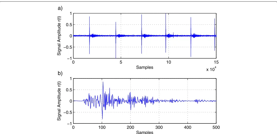
Figure 1Impulsive acoustic source signal generated by a toy gun shot.(a)Multiple instances of an impulsive source signal generated by a toy gun fire.(b)Single instance of an impulsive source signal generated by a toy gun fire.
30 kHz. Figure 1a shows several instances of the gunshot signal, while Figure 1b zooms into one of the instances to show the signal shape.
Note that we are only concerned withFM(i.e., the
sub-sampling frequency) and not with FS. The only
require-ment for the proposed method to work is thatFM < T1
to make sure that the gunshot is not missed completely during sub-sampling.
6.2 TDE simulation results
The performance of the OC-based TDE method is ana-lyzed in simulations by creating a virtual room environ-ment. The impulse response of the channel between a source-microphone pair placed in a room with specific dimensions is obtained using an image-source model as presented in [31]. Figure 2 shows the shoe box model of a room with dimensions 8×6×3 m (x×y×z).
0
2
4
6
8
0 2
4 6
0 0.5 1 1.5 2 2.5 3
Room Length Sensor
Source
Room Width
Room Height
0 10 20 30 40 50 −1
0 1
Room Impulse Response (b)
Time (ms)
Amplitude
0 10 20 30 40 50
−1 0 1
Source Signal (a)
Time (ms)
Amplitude
0 10 20 30 40 50
−1 0 1
Received Signal (c)
Time (ms)
Amplitude
Figure 3Typical impulsive acoustic source signal (a), room impulse response (b), and received signal at the microphone (c).
Two reverberant environments are considered with different extent of reverberations. A dense reverberant environment is created by setting high wall reflection coefficients, ([x1 = 0.75,x2 = 0.75,y1 = 0.8,y2 = 0.8,z1 = 0.85,z2 = 0.9]). For a less reverberant envi-ronment, the reflection coefficients are set low ([x1 = 0.2,x2 = 0.2,y1 = 0.3,y2 = 0.25,z1 = 0.3,z2 = 0.5]). Note that these values are selected to mimic the two extreme room environments, and any other values could
have been used. The reverberation timeT60is set to 0.25 s, whereT60is the time it takes for the signal energy to fall below−60 dB.
The sampling frequency of the microphones is ini-tially set to 10 kHz. Figure 3a shows a typical impulsive source signal (a recorded toy gun shot). The room impulse response generated using the model in [31] is shown in Figure 3b. The signal received at the microphone is the convolution of source signal with the RIR as shown
0 10 20 30 40 50
−1 −0.8 −0.6 −0.4 −0.2 0 0.2 0.4 0.6 0.8 1
Time (ms)
Normalized Amplitude
Actual RIR Estimatated RIR
0 10 20 30 40 50 −1
−0.8 −0.6 −0.4 −0.2 0 0.2 0.4 0.6 0.8 1
Time (ms)
Normalized Amplitude
Actual RIR Estimatated RIR
Figure 5Example of simulated RIR estimation (dense reverberations).
in Figure 3c. The sparsity of the RIR is observable in Figure 3b.
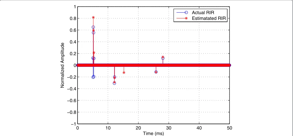
An example of the RIR estimation for a low reverber-ant room environment is shown in Figure 4. The OC algorithm is applied for the sparse RIR estimation with sampling rate of 8 kHz. The direct path signal and most of the reflected signals are correctly estimated while few early reflections are missed. Figure 5 shows an example
of a dense reverberant environment. Here, the direct path signal is accurately estimated as well as a number of early and late reflections.
Figure 6 demonstrates the performance of the OC algo-rithm for different sub-sampling rates. For simulation purpose, the signal-to-noise ratio (SNR) is set by adding mutually independent white Gaussian noise to the acquired microphone signal to control the SNR. The
2 3 4 5 6 7
−60 −50 −40 −30 −20 −10 0
Sub−sampling rate (F s/Fm)
MSE in Time−Delay Estimation (dB)
High Reflection Coefficients (SNR=30dB) Low Reflection Coefficients (SNR=30dB) High Reflection Coefficients (SNR=40dB) Low Reflection Coefficients (SNR=40dB)
Figure 7Experimental setup for indoor TDE.
simulation is run for 500 iterations for two values of SNR, 30 and 40 dB, respectively. For each iteration, the posi-tion of the microphones and the acoustic source were randomly varied within the room boundaries, and RIR is generated using the image source model in [31]. It can be seen that for the 40-dB case, the MSE at low sub-sampling rates is quite low and the performance degrades gradually for higher sub-sampling rates, while there is a significant degradation in performance for sub-sampling rate greater
than 2 in the 30-dB case. With less measurements (high sub-sampling factor), the performance of the OC-based RIR reconstruction degrades which eventually results in increased MSE in TDE. Thus, the OC algorithm requires more measurements to estimate the sparse RIR at low values of SNR.
6.3 TDE experimental results
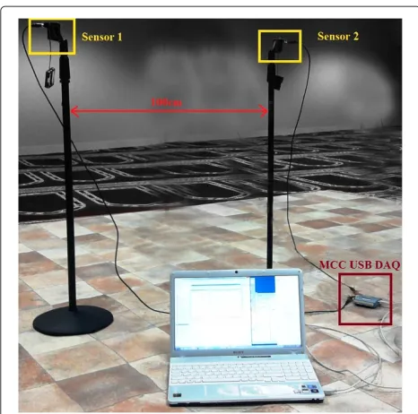
Figure 7 shows the actual hardware setup for TDE in a
hall room of dimensions 8×6×3 m. Two microphones
are secured with metallic stands placed 100 cm apart. The electret microphones are mounted on low-noise ampli-fier (LNA) PCBs with a MAX 9814 LNA IC whose gain is set to 40 dB. The output of the LNAs are connected to a 16-bit, 8-channel data acquisition (DAQ) device via audio jacks and cables. The DAQ communicates with a PC through the data acquisition tool box within MATLAB. The DAQ device is configured using MATLAB com-mands to acquire uniform samples of the source signal at the sampling rates ofFM =16, 8, and 4 kHz,
respec-tively. A toy gun was used as the impulsive source with a duration of approximately 10 ms as shown in Figure 3. From the figure, the experimental value of the SNR is determined by taking the ratio of the signal varianceσs2 (portion of the waveform that corresponds to the gun shot signal) and the noise varianceσn2(portion of the waveform that corresponds to the background noise received at the microphone). The SNR is determined from the following expression:
SNR=10 log10
σs2 σ2
n
(19)
Figure 9Experimental RIR estimate with microphone close to the wall.
The average SNR value in the experiments was SNR ≈
20 dB. The dictionary matrix in (4), required for the RIR estimation using the OC algorithm, is constructed by averaging several instances of the impulsive source sig-nal at FS = 16 kHz whereFS = FM (i.e., sub-sampled
frequency) as introduced before.
The first step in finding the time delay based on the proposed OC method is to estimate the sparse RIR. To illustrate this intermediate step of RIR estimation, we discuss two instances of the RIR estimated for different microphone positions inside the room. In the first case, the microphone is placed at the room center and with the source lying close to it. The estimated RIR shows the direct path, early reflections along with few late reflec-tions as shown in Figure 8. Thus, we observe that the effect of room reverberations is quite low when microphone is placed away from sound obstacles (room walls). Another example of RIR estimation is conducted with the micro-phone placed close to the room walls. The estimated RIR contains a direct path along with a number of reflections as shown in Figure 9. The presence of the walls close to the microphone builds dense reverberations. This effect is apparent in the high number of room reflections of the estimated RIR.
The real-time functionality of the algorithm for TDE has been verified by placing the source at known locations around the microphones and acquiring the source signal at various sampling rates. Table 1 shows the time delays corresponding to three known source locations:
1. Case I: source positioned at a point on the line that passes through the two microphones.
2. Case II: source positioned close to microphone 1, on the vertex of an isosceles triangle formed by the microphones and the source.
3. Case III: source positioned in the middle of the line joining the two microphones.
The corresponding estimated time delays using CC and the proposed algorithm for three sampling rate values of FM=16, 8, and 4 kHz are shown in Table 1. The sampling
rates are selected by setting the data acquisition hardware to the desired rate. It can be seen that the proposed algo-rithm gives closer time delay estimates when compared to CC in the case of low sampling rates. This demonstrates the superior performance of the OC-based technique used
Table 1 Comparison of time delay estimates obtained using CC and the proposed technique based on OC algorithm
Frequency True TD TDE CC Run time TDE OC Run time (kHz) (ms) (ms) CC (s) (ms) OC (s)
Case I 16 2.941 2.875 66 2.875 70
8 2.941 3.125 17 2.875 7
4 2.941 2.250 4.5 3.312 3.5
Case II 16 1.218 1.250 66 1.250 70
8 1.218 0.875 17 1.312 7
4 1.218 1.000 4.5 1.250 3.5
Case III 16 0.000 0.000 66 0.000 70
8 0.000 0.250 17 0.000 7
Figure 10Microphone configuration I for source localization.(a)Configuration geometry.(b)Experimental setup.
in [19] when tuned to work for this application. In addi-tion, the run time needed to provide TDE of the proposed algorithm are faster than CC at low sampling rates, which gives it a computational advantage as well.
6.4 Source localization results
In this sub-section, we present the results of time delay-based localization experiment. The inherent limitations of DOA-based localization method specifically for indoor environment and under low sampling rate are initially dis-cussed. We apply the TDOA method for localization as it suits our application. Results of several localization exper-iments for three different microphones geometries are presented.
6.4.1 DOA-based source localization
The TDE is an integer multiple of the sampling period
Ts in the absence of an interpolation technique. The
estimated delays suffer from poor time resolution at low sampling frequencies (large sampling period) [5]. Such low time resolution is not suitable for DOA-based local-ization scheme where the spatial resolution between the microphones (inter-microphone spacing) is also low. Con-sider a setup for DOA estimation consisting of an array of two microphones separated by a small distancedand a source that lies in the far field of the array. The bear-ing angle θ is related to the time delay, which for 1D microphone array is expressed as [6]
θ =cos−1cτ d
(20)
wherecis the sound propagation velocity.
The angular resolution of an array determines the num-ber of different DOA measurements between 0 andπ. It directly corresponds to the sampling frequencyFs
(sam-pling time Ts). For instance, a microphone array, with
−200 −150 −100 −50 0 50 100 150 200 −200
−150 −100 −50 0 50 100 150 200
x co−ordinate (cm)
y co−ordinate in (cm)
Sensor Loc.
Source Loc. (−100,100) Est. Loc. (Fs=8KHz) Est. Loc. (Fs=4KHz)
a 30-cm inter-microphone spacing, can provide only 14 distinct DOA measurements at the sampling frequency Fs = 16 kHz, 7 measurements atFs = 8 kHz and 4
mea-surements atFs=4 kHz between 0 andπ, respectively.
Increasing the sampling rate improves the TDE reso-lution which in turn lead to a higher DOA resoreso-lution [5]. However, this approach will increase the complex-ity of both the TDE algorithm and hardware. Other ways to improve the DOA resolution is by increasing
micro-phone spacing dN which will increase the size of the
array. Also, the far field requirement for DOA estimation makes it hard to implement in a room environment with a limited space. Moreover, large microphone spacing may
cause spatial aliasing. It may also lead to higher computa-tional complexity since more data has to be acquired for extended time durations to account for the larger delay range.
6.4.2 TDOA-based source localization
Time difference of arrival (TDOA) is another widely used TDE-based source localization method. The method is a two-step procedure. In the first stage, the time difference of signal arrival between a pair of microphones is esti-mated. With the knowledge of the propagation velocity of sound, the estimated TDOA measurement is transformed into range difference measurement from which hyperbolic
Table 2 Microphone configuration I results for the source location of (−100, 100)
Fs True time Estimated tau Estimated source Run time Estimated tau Estimated source Run time
delay CC location CC CC OC location OC OC
(kHz) (ms) (ms) (cm) (s) (ms) (cm) (s)
4.250 3.125
1.250 L.F. −0.625 L.F.
1.250 −0.625
2.125 2.375
−1.250 (−39.3, 78.1) −0.937 (−61.8, 76.2)
−2.250 −0.375
2.417 4.500 2.375
8 −1.218 −1.125 L.F. 17 −1.250 (−88.1, 96.5) 7
−1.218 −1.0000 −1.000
4.250 2.312
−1.000 L.F. −1.375 (−82.6, 99.5)
−7.250 −0.812
2.125 2.062
−1.500 (−49.7, 89.0) −1.562 (−43.4, 88.0)
−0.250 0.187
1.250 2.250
−2.750 (−0.1, 96.7) −1.500 (−77.9, 102.7)
−2.500 −0.687
2.500 3.650
−1.500 L.F. −1.562 L.F.
−2.000 −0.500
2.417 −0.750 2.125
4 −1.218 −1.750 (83.3, 118.8) 4.5 −1.250 (−39.2, 78.1) 3.5
−1.218 −1.250 0.312
3.650 2.562
−0.750 L.F. −0.687 (−89.0, 74.3)
−1.250 −1.187
2.250 2.500
−0.500 (−30.2, 60.0) −0.812 (−80.3, 76.8)
−0.500 −0.937
range difference equation is formed. The second stage utilizes efficient algorithms to produce an unambiguous solution to the hyperbolic equations obtained from multiple microphone pairs. The solution produced by these algorithms result in the estimated source location.
The drawbacks of DOA method for indoor localiza-tion made us focus on using the TDOA-based localizalocaliza-tion method. The TDOA-based method does not make the far field assumption (i.e., plane waves arriving at micro-phones). Moreover, the microphones can be separated by large distances that provides higher spatial resolution for TDE at low sampling frequencies. In the following, we consider three different microphone geometries. For each geometry, we apply the CC and OC algorithms for TDE and apply the TDOA method for two-dimensional (2D) source localization.
6.4.3 Microphone configuration I
The microphone configuration shown in Figure 10a con-sists of a 2D microphone array placed in the xy plane. MicrophoneM1 placed at the center of the array is taken as a reference of the array. The location of the reference microphoneM1 defines the origin (intersection ofxand yaxis) of the 2D plane. Other microphonesM2,M3, and
M4 are placed at an equidistant spacing of d = 100
cm from the reference shown in Figure 10. The TDOA-based localization in 2D plane requires a minimum of two time delay estimates obtained from three microphones where the two TDEs corresponds to the two microphone pairsM1,M2 andM1,M3, respectively. However, adding
an extra microphone M4 gives a redundant time delay
measurement which can be used to improve the location estimate.
The experimental setup for microphone configuration I is shown in Figure 10b. The setup is made on a 4×4 m
floor mat placed in the room center. The floor mat has a
printed grid of 20×20 cm which helps in microphones
and source placement. The acoustic sensors are secured on top of metallic stands. The height of the stands form a 2D plane in which the acoustic source lies (a person fir-ing a gun). Outputs of the pre-amplifiers are connected via audio leads and jacks to four different channels on a USB data acquisition device. MATLAB is used for data acquisition and further signal processing for the source localization algorithm.
The CC- and OC-based methods of TDE have been applied on the data acquired for different source locations. In order to assess the consistency of both algorithms, five instances of the source signal are acquired at each source location at sampling rates of 4 and 8 kHz, respectively. TDOA-based source localization is used to determine the source location based on the estimated time delays.
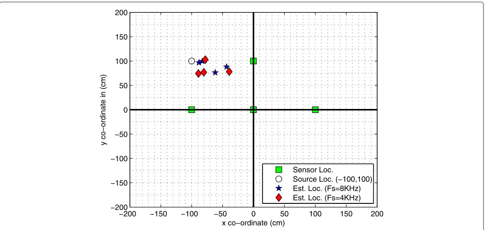
The estimated locations using the proposed OC method (with sub-sampling), for the source positioned at vari-ous locations in the vicinity of the acvari-oustic sensors, were recorded for five different source locations. Figure 11 shows one of the positions where the source was at (−100, 100) cm. The figure shows the position of the microphones (filled squares), source location (hollow cir-cles), and the estimated source locations (stars for 8 kHz and diamond for 4 kHz). The plot area represents the region of the floor mat. It can be observed that the source locations for the 8-kHz measurements lie in close prox-imity to the true location. The location estimates for the 4-kHz measurements are observed to be lying rel-atively farther from the true source location than with the 8-kHz measurements. This shows the trade off that exists between the accuracy of location estimates and the sub-sampling rates as shown earlier in Figure 6.
The experimental results of the CC- and OC-based time delay and source location estimates for microphone
Figure 13Microphone configuration II for source localization.(a)Configuration geometry.(b)Experimental setup.
configuration I with source location (−100, 100) cm are also tabulated in Table 2. The table provides the results of the estimated time delays, source location, and computa-tion time of both TDE techniques for this specific source location sampled at two different sampling rates. Five dif-ferent locations were examined for this geometry. Tables similar to Table 2 were generated for each case. From the results of this configuration, we conclude that
• The benefit of the proposed method becomes obvious
when the source signal is sub-sampled. With the 8-kHz measurements, the proposed OC-based TDE method gives better and more consistent location estimates as compared to the CC which fails (location failure (LF)) several number of times to locate the source in an
acceptable region (4×4 m). Figure 12 shows that CC fails2more than 50% of the times, while the failure rate of OC is less than 30%. The OC algorithm computes TDE in 7 s which is much less than 17 s taken by CC.
• Sampling the source signal at even lower rate of 4 kHz deteriorates the performance of the CC method to a much larger extent, resulting in an increased percentage of localization failures up to 85%. In contrast, OC gives acceptable location estimates in many cases with rela-tively less percentage, 40% of localization failures. The computation time of OC is 3.5 s which is less than 4.5 s taken by CC.
The acoustic source used is not an ideal point source, but in fact, it is a person exciting an acoustic source
0 50 100 150 200 250 300 350 400 0
50 100 150 200 250 300 350 400
x co−ordinate (cm)
y co−ordinate in (cm)
Sensor Loc.
Source Loc. (100,200) Est. Loc. (Fs=8KHz) Est. Loc. (Fs=4KHz)
while standing at the true location. Hence, we expect the location estimates to lie within an area around the source (±25 cm).
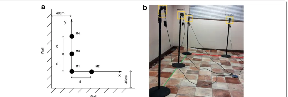
6.4.4 Microphone configuration II
Another microphone configuration examined for the source localization experiments is shown in Figure 13. It consists of a 2D microphone array placed in anxyplane.
Microphone M1 is taken as an array reference and is
placed at the origin. MicrophonesM2 andM3 are placed at an equidistant spacing ofd = 100 cm from the refe-rence along the horizontal and vertical axis, respectively. MicrophoneM4 is placed 200 cm apart from the reference
along theyaxis. The fourth microphoneM4 provides an extra time delay measurements which in turn improves the location estimates. This array was placed at the room corner to obtain more reverberations.
The proposed OC-based method and the CC method were applied on the acquired data for three different source locations. For each source location, the signal was acquired at sampling rates of 4 and 8 kHz, respec-tively. The location estimates for the source positioned at (100, 200)cm are shown in Figure 14.
From the figure, we observe that with the sampling rate of 8 kHz, a high percentage of estimated source locations are in close proximity with the true location. Decreasing
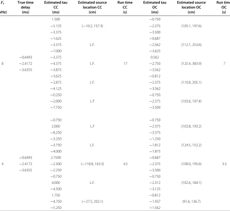
Table 3 Microphone configuration II results for the source location of (100, 200)
Fs True time Estimated tau Estimated source Run time Estimated tau Estimated source Run time
delay CC location CC CC OC location OC OC
(kHz) (ms) (ms) (cm) (s) (ms) (cm) (s)
1.500 −0.750
−5.125 (−10.2, 157.3) −2.375 (105.1, 197.6)
−3.375 −3.500
−1.625 −0.687
−3.375 L.F. −2.562 (112.1, 253.6)
−7.000 −3.625
−0.6493 −3.375 0.562
8 −2.4172 −4.375 L.F. 17 −2.750 (125.4, 383.9) 7
−3.6355 −3.875 −3.562
−3.625 −0.812
−2.875 L.F. −2.375 (110.8, 205.1)
−4.125 −3.562
−0.250 −0.750
−2.000 L.F −2.375 (103.6, 197.4)
−7.750 −3.500
−0.750 −0.750
2.000 L.F −2.375 (102.8, 193.2)
−8.250 −3.375
−3.250 −1.250
−3.750 L.F. −1.812 (124.5, 152.2)
−4.000 −1.875
−0.6493 2.7500 −0.687
4 −2.4172 −2.500 (−118.8, 163.3) 4.5 −2.375 (100.0, 195.6) 3.5
−3.6355 −2.250 −3.500
−0.750 −0.750
4.000 L.F. −2.312 (102.6, 184.1)
−4.500 −3.125
1.750 −0.812
−4.750 (−27.5, 202.1) −1.937 (91.6, 136.7)
−5.250 −1.562
the sampling frequency to 4 kHz, the algorithm finds close location estimates in many cases, while in others, the esti-mates lie a bit far from the true location. Tabulated results are shown in Table 3. We make the following observations from the results obtained:
• The close to wall microphone configuration results in an increased level of room reverberations. At 8 kHz, the proposed OC-based method is observed to be working effectively under dense room reverberation conditions. Comparing this case with the center room configura-tion, the localization failure has significantly decreased from 30% to 12%. In contrast, the CC method suf-fers both from the increased level of reverberations and higher under-sampling factors. These reverbera-tions result in an increased rate of localization failures from 50% (center room configuration) to 60%. A com-parison of localization failures of both CC and OC with respect to the sampling frequencies is shown in Figure 15. Moreover, the execution time of OC method is 7 s which is much faster than 17 s consumed by CC.
• At 4 kHz, the OC method performs consistently well
under high sub-sampling rate with a low percentage 20% of localization failures as compared to 40% for center room configuration. On the other hand, the per-formance of the CC method deteriorates further at such low sampling rate. A high percentage of localization failures of more than 75% are observed with CC. The computation time of OC is 3.5 s, faster than 4.5 s of CC.
6.4.5 Microphone configuration III
Figure 16 shows the third microphone configuration for the source localization experiments. It represents a 2D microphone array placed in anxyplane. MicrophoneM1 is taken as an array reference and is placed at the origin.
Microphones M2 and M3 are placed at an equidistant
spacing of d = 100 cm from the reference along the
horizontal and vertical axis respectively. MicrophoneM4 is placed 100 cm apart from the reference in bothxandy axes. The fourth microphoneM4 provides an extra time delay measurements which in turn improves the location estimates. This geometry was also built next to the wall to increase reverberations.
The estimated locations for the source position at location (200, 100) cm are shown in Figure 17. Table 4 shows all the experimental results conducted for micro-phone configuration III. From the results, we observe the following:
• At 8 kHz, the OC method works better under increased level of reverberations as less localization failure rate of10%is observed as compared to30% for center room configuration. Once again, we observe performance degradation of CC method with high failure rate of CC of60%caused by increased reverberations and high under sampling factor. Figure 15 shows the comparison between the localization failures of OC and CC under different sampling rates. The execution time of OC method is 7 sec which is much less than 17 s consumed by CC.
• At 4 kHz, the OC method performs effectively under dense reverberations. Comparing with center room configuration, less localization failure rate of20%is achieved. In contrast, CC fails to locate the source 70%of the times due to high sub-sampling rate and increased reverberations. Figure 18 shows the rate of localization failure for both OC and CC methods under different sub-sampling rates. The computation time of OC is 3.5 s, faster than 4.5 s of CC.
7 Discussion
The time delays for an indoor environment are extremely small (few milliseconds), where the source and the
Figure 16Microphone configuration III for source localization.(a)Configuration geometry.(b)Experimental setup.
microphones lie close to each other. In this case, accu-rate TDE requires high time resolution (low sampling time). The proposed method reconstructs a sparse RIR signal using signal statistics, sparsity information, and the problem structure. Although decreasing the number of measurements (sampling rate) makes the RIR estimation less accurate, this does not decrease the time resolution. In contrast, CC-based TDE method depends largely on the sampling rate. At low sampling rates, the time reso-lution (large sampling time) becomes poor which makes it hard to find the correlation peak close to the true time delay.
The proposed method estimates the time delays from the RIR. The accuracy of TDE depends largely on estimating the impulse which corresponds to the direct path signal. Since RIR is estimated from under-sampled signal, there is a possibility to miss the impulse corre-sponding to the true time delay. The TDE in such case will rely on estimating the closest reflection. Thus, increased level of reverberations in the close wall configuration favored the proposed TDE method as it suffered from low localization failures as compared to the center room configuration. On the other hand, reverberations have an adverse effect on CC method. The reflected signals cause
0 50 100 150 200 250 300 350 400 0
50 100 150 200 250 300 350 400
x co−ordinate (cm)
y co−ordinate in (cm)
Sensor Loc.
Source Loc. (200,100) Est. Loc. (Fs=8KHz) Est. Loc. (Fs=4KHz)
Table 4 Microphone configuration III results for the source location of (200, 100)
Fs True time Estimated tau Estimated source Run time Estimated tau Estimated source Run time
delay CC location CC CC OC location OC OC
(kHz) (ms) (ms) (cm) (s) (ms) (cm) (s)
−5.500 −3.437
−2.625 L.F. −3.250 (193.3, 98.3)
0 −0.125
−5.500 −3.562
−2.000 L.F. −3.625 (199.8, 103.8)
−3.250 −0.125
−3.635 −5.500 −3.500
8 −3.635 −3.375 L.F. 17 −3.750 (190.8, 93.8) 7
0 7.375 0.250
−5.500 3.500
−3.125 (298.3, 67.4) −3.000 (195.5, 96.7)
0.625 0.187
−6.875 −3.500
−3.375 (310.3, 15.4) −3.562 (194.5, 98.7)
2.000 0
−5.750 −3.625
−3.500 L.F. −3.625 (193.4, 90.4)
−4.250 0.312
−5.500 −3.625
−3.750 L.F. −3.500 (200.3, 100.1)
0.500 −0.062
−3.635 −5.500 −3.500
4 −3.635 −4.000 L.F. 4.5 −4.000 (208.5, 123.7) 3.5
0 −5.750 −0.562
−3.250 −3.312
−7.000 L.F. −3.562 (189.1, 100.4)
−2.250 −0.062
−3.000 −3.250
−4.250 L.F. −3.312 (188.2, 100.9)
−3.750 −0.187
L.F., localization failure.
multiple peaks to appear in the correlation resulting in performance degradation.
Increase in the sampling rate improved the perfor-mance of OC-based TDE method, as more measure-ments favored the sparse RIR signal reconstruction. Thus, OC-based localization method performed better at the sampling rate of 8 kHz (localization failure ≤ 30%) as compared to 4 kHz (localization failure≤40%).
Placing the microphones close to the wall improved the performance of the proposed OC-based method. Among the three microphone configurations that we experimented, the least localization failures (≤20%) were experienced with the microphone configuration II. Simi-lar failure rate was observed in microphone configuration
III, while the center room configuration resulted in a large rate of localization failure (≤40%).
8 Conclusions
Figure 18Localization failures in CC and OC for microphone configuration III.
the localization process computationally intensive and imposes the need for sophisticated hardware. Moreover, the need of centralized processing in CC-based methods puts strain on the communication link between sensors and the processing unit. This motivated us to develop a more robust TDE method, based on the RIR estima-tion to enhance the robustness of indoor acoustic source localization. In addition, the proposed method works at extremely low sampling rates and hence decreases the computation time and hardware complexity. More-over, the distributed nature of the proposed algorithm enables it to perform localization at the sensor level which eliminates the need for centralized processing. The performance of the proposed method for TDE and local-ization is analyzed by both simulations and experimen-tal setup. The results show the improved performance of the proposed method over the existing CC method. Several microphone configurations are considered for source localization experiments. Through experimen-tal evidences and theoretical understanding, it is found that the close wall configuration favored the proposed method.
Endnotes
1Note that it is necessary for the sub-sampling ratio to
be less thanTto avoid missing the source signal completely, i.e.,FMshould be less thanT1. Ideally
speaking, the gunshot will have frequency≥20 kHz being an acoustic signal of impulsive nature.
2Localization failure is the ratio of the number of times
the algorithm fails to locate the source in an acceptable region to the total number of measurements conducted at a specificFs.
Competing interests
The authors declare that they have no competing interests.
Acknowledgements
The authors would like to acknowledge the support provided by the King Abdulaziz City for Science and Technology (KACST) through the Science and Technology Unit at King Fahd University of Petroleum and Minerals (KFUPM) for funding this work through project no. 09-ELE763-04 as part of the National Science, Technology and Innovation Plan.
Author details
1Electrical Engineering Department, King Fahd University of Petroleum &
Minerals, Dhahran 31261, Saudi Arabia.2Electrical Engineering Department,
King Abdullah University of Science and Technology (KAUST), Thuwal 23955, Saudi Arabia.
Received: 22 December 2013 Accepted: 26 June 2014 Published: 22 July 2014
References
1. G Carter, A Nuttall, P Cable, The smoothed coherence transform. Proc. IEEE.61, 1497–1498 (1973)
2. J Ianniello, Time delay estimation via cross-correlation in the presence of large estimation errors. IEEE Trans. Acoustics Speech Signal Process. 30, 998–1003 (1982)
3. G Jacovitti, G Scarano, Discrete time techniques for time delay estimation. IEEE Trans. Signal Process.41, 525–533 (1993)
4. MS Brandstein, Time-delay estimation of reverberated speech exploiting harmonic structure. J. Acoust. Soc. Am.105, 2914 (1999)
5. J Chen, J Benesty, YA Huang, Time delay estimation in room acoustic environments an overview. EURASIP J. Adv. Signal Process.2006, 1–20 (2006)
6. B Berdugo, MA. Doron, J Rosenhouse, H Azhari, On direction finding of an emitting source from time delays. J. Acoust. Soc. Am.105, 3355 (1999) 7. U Klee, T Gehrig, J McDonough, Kalman filters for time delay of
arrival-based source localization. EURASIP J. Adv. Signal Process.2006, 1–16 (2006)
8. PB Muanke, C Niezrecki, Manatee position estimation by passive acoustic localization. J. Acoust. Soc. Am.121, 2049–59 (2007)
9. Y Teshima, J-y Takayama, S Ohyama, K Oshima, Person localization using TDOA of non-speech sound signal based on multiplexed CSP analysis, in Proceedings of SICE Annual Conference 2010(Taipei, 18–21 Aug 2010) 10. T Han, X Lu, Q Lan, Pattern recognition based Kalman filter for indoor
localization using TDOA algorithm. Appl. Math. Model.34, 2893–2900 (2010)
11. Y Chan, K Ho, A simple and efficient estimator for hyperbolic location. IEEE Trans. Signal Process.42, 1905–1915 (1994)
13. C Knapp, G Carter, The generalized correlation method for estimation of time delay. IEEE Trans. Acoustics Speech Signal Process.24, 320–327 (1976)
14. B Champagne, S Bedard, A Stephenne, Performance of time-delay estimation in the presence of room reverberation. IEEE Trans. Speech Audio Process.4, 148–152 (1996)
15. J Chen, J Benesty, YA Huang, Performance of GCC- and AMDF-based time-delay estimation in practical reverberant environments. EURASIP J. Adv. Signal Process.2005, 25–36 (2005)
16. J Benesty, Adaptive eigenvalue decomposition algorithm for passive acoustic source localization. The J. Acoust. Soc. Am.107, 384–392 (2000) 17. OM Bouzid, GY Tian, J Neasham, B Sharif, Investigation of sampling
frequency requirements for acoustic source localisation using wireless sensor networks. Appl. Acoustics.74(2), 269–274 (2013)
18. AA Quadeer, SF Ahmed, TY Al-Naffouri, Structure based Bayesian sparse reconstruction using non-Gaussian prior, in49th Annual Allerton Conference on Communication, Control, and Computing (Allerton) (Monticello, Sept 2011), pp. 277–283
19. TY Al-Naffouri, AA Quadeer, G Caire, Impulsive noise estimation and cancellation in DSL using orthogonal clustering, in2011 IEEE International Symposium on Information Theory Proceedings(St. Petersburg, Aug 2011), pp. 2841–2845
20. AA Quadeer, TY Al-Naffouri, Structure-based Bayesian sparse reconstruction. IEEE Trans. Signal Process.60, 6354–6367 (2012) 21. R Ratnam, DL Jones, BC Wheeler, WD O’Brien, CR Lansing, AS Feng, Blind
estimation of reverberation time. J. Acoust. Soc. Am.114, 2877–92 (2003) 22. M Duarte, M Davenport, D Takhar, J Laska, K Kelly, R Baraniuk, Single-pixel imaging via compressive sampling. IEEE Signal Process. Mag.25, 83–91 (2008)
23. M Lustig, D Donoho, JM Pauly, Sparse MRI: The application of compressed sensing for rapid MR imaging. Magn. Reson. Med.58, 1182–95 (2007) 24. J Haupt, WU. Bajwa, G Raz, R Nowak, Toeplitz compressed sensing
matrices with applications to sparse channel estimation. IEEE Trans. Inf. Theory.56, 5862–5875 (2010)
25. JL Paredes, GR Arce, Z Wang, Ultra-wideband compressed sensing: channel estimation. IEEE J. Selected Top. Signal Process.1, 383–395 (2007) 26. G Leus, A Pandharipande, Direction estimation using compressive
sampling array processing, in2009 IEEE/SP 15th Workshop on Statistical Signal Processing(Cardiff, Sept 2009), pp. 626–629
27. M Herman, T Strohmer, High-resolution radar via compressed sensing. IEEE Trans. Signal Process.57, 2275–2284 (2009)
28. EJ Candès, JK Romberg, T Tao, Stable signal recovery from incomplete and inaccurate measurements. Commun. Pure Appl. Math. 59, 1207–1223 (2006)
29. J Tropp, Just relax: convex programming methods for identifying sparse signals in noise. IEEE Trans. Inf. Theory.52, 1030–1051 (2006)
30. EJ Candes, PA Randall, Highly robust error correction by convex programming. IEEE Trans. Inf. Theory.54, 2829–2840 (2008)
31. EA Lehmann, AM Johansson, Prediction of energy decay in room impulse responses simulated with an image-source model. J. Acoust. Soc. Am. 124, 269–77 (2008)
doi:10.1186/1687-6180-2014-116
Cite this article as:Omeret al.:Sub-sampling-based 2D localization of an impulsive acoustic source in reverberant environments.EURASIP Journal on Advances in Signal Processing20142014:116.
Submit your manuscript to a
journal and benefi t from:
7Convenient online submission 7Rigorous peer review
7Immediate publication on acceptance 7Open access: articles freely available online 7High visibility within the fi eld
7Retaining the copyright to your article