R E S E A R C H
Open Access
Optimum beamforming for MIMO multicasting
Baisheng Du
1*, Yi Jiang
2, Xiaodong Xu
1*and Xuchu Dai
1Abstract
This paper investigates the transmit (Tx) beamforming design to maximize the throughput of a multiple-input multiple-output multicast channel, where common information is sent from the base station toKusers
simultaneously. This so-called max-min fair beamforming problem is known to be NP-hard. When the base station is equipped with two Tx antennas, we prove that the original complex-valued beamforming problem can be
transformed into a real-valued problem and the globally optimal solution can be found by exhausting at most
C1K+CK2+C3Khypothesis tests. Moreover, a prune and search algorithm (PASA) is proposed for searching the optimal beamformer with computational complexityO(K3)in the worst case. When the base station has more than two Tx antennas, we develop an efficient algorithm named iterative two-dimensional optimization which converts the original beamforming problem into a series of two-antenna subproblems by iterations and hence, the beamformer is improved using PASA iteratively. Simulations results are presented to demonstrate the superior performance of the proposed algorithms.
Keywords: Physical layer multicasting; Multiple-input multiple-output; Transmit beamforming; Semidefinite relaxation (SDR)
1 Introduction
In the next generation of wireless networks, spectrally efficient multicasting techniques are required to support applications such as web TV, online gaming, and software updates, where common messages are sent to a group of users simultaneously. Under the assumption that the channel state information of all users is available at the multi-antenna base station (BS), transmit (Tx) beamform-ing can be used to improve the performance of multicast-ing. Consequently, the problem of multicast beamforming has received significant attentions recently[1-5].
In [1], Lopez formulated the multicast beamforming problem as maximizing the average signal-to-noise ratio (SNR) of all users, for which the optimal beamformer can be obtained by an eigendecomposition. However, this approach does not guarantee satisfactory performance for all users. In general, the performance of multicasting is determined by the user(s) with the lowest SNR. From this point of view, a practical criterion is to maximize the minimal SNR of all users. This optimization problem is referred to as max-min fair beamforming and is known
*Correspondence: [email protected]; [email protected]
1Department of Electronic Engineering and Information Science, University of Science and Technology of China, Hefei, Anhui 230027, China
Full list of author information is available at the end of the article
to be NP-hard. The seminal work of max-min fair beam-forming is proposed in [2], where semidefinite relaxation (SDR) is used to yield approximate solutions. In order to achieve higher throughput or reduce the implementation complexity, various iterative schemes are proposed subse-quently. In [3], the closed-form expression of the optimal beamformer is deduced for the two-user case. For the case of more than two users, a group of beamformers are calculated through different pairs of users by the closed-form expression. Then, the best one among these beam-formers is used to be an initialization for the proposed iterative algorithm, whose main idea is to improve the lowest SNR at each iteration. Furthermore, it is showed that this method is computationally much simpler while the performance is comparable to that of the SDR-based scheme. In [4], another iterative approach based on chan-nel orthogonalization and local refinement is developed, and it provides attractive performance compared to the methods in [2] and [3]. Similar to [3], the authors in [5] also develop a closed-form solution for the beamformer design, wherein two users are assumed. Then, a succes-sive greedy algorithm based on the two-user case are proposed to tackle the general cases. Recently in [6], the authors consider the robust design for unicast downlink beamforming and conclude that the optimal beamforming
vectors can be obtained by the semidefinite relaxation when the base station is equipped with two antennas. Yet, it cannot be applied to the multicast scenario we investigate here.
For the max-min fair beamforming problem, to the best of our knowledge, previous methods are not guaranteed to obtain the globally optimal beamforming vector when the base station serves arbitrary number of users. In addition, most of the methods are only applicable to the scenario of single-antenna users. In this paper, we intend to address the general case for max-min fair beamforming where the users are equipped with one or multiple receive antennas. The main contributions of this paper are listed below:
(1) For the case that the BS has two Tx antennas, we derive that the feasible set of the SNR vector of all users is a two-dimensional ellipsoid in
K -dimensional Euclidean space, where K is the number of users. With this geometrical property, we prove that the original complex-valued optimization problem can be simplified as a real-valued problem and the optimal beamforming vector can be found by exhaustingC1K+C2K+CK3 hypothesis tests of the bottleneck users, which are defined as the users with the lowest SNR.
(2) In order to reduce the complexity of exhausting, we propose a prune and search algorithm (PASA) which is guaranteed to find the globally optimal
beamformer. By analyzing the probabilities for three cases of bottleneck users, we prove that the
worst-case computational complexity of PASA is O(K3). It is showed that PASA is computationally more efficient than most of the existing schemes. (3) For the general case that the BS is equipped with
more than two Tx antennas, we propose an iterative two-dimensional optimization (I2DO) algorithm which iteratively transforms the problem of beamformer design into a sequence of two-antenna subproblems and then PASA can be used to improve the beamformer at each iteration. When the number of users is large, the throughput achieved by the proposed beamformer has considerable improvement over the state-of-the-art multicasting techniques.
The remainder of this paper is organized as follows. In Section 2, we introduce the input multiple-output (MIMO) multicast channel and formulate the transmit beamforming problem. In Section 3, we ana-lyze the special case of two Tx antennas and deduce a new formulation for the beamformer design. Based on the new formulation, the PASA is proposed to obtain a glob-ally optimal beamforming vector. For the case of more than two Tx antennas, we propose the I2DO algorithm in Section 4. Section 5 presents simulation results to verify
the effectiveness of the proposed approaches. Finally, conclusions are drawn in Section 6.
Notations: We use uppercase and lowercase bold let-ters to denote matrices and vectors. The superscripts(·)T, (·)∗, and (·)† stand for transpose, conjugate transpose, and pseudo-inverse, respectively. Re(·) and Im(·) mean the real part and imaginary part, respectively. · and ·Fdenote the vector Euclidean norm and the Frobenius
norm.Inrepresents ann×nidentity matrix and1nis an
all-one column vector with lengthn, while0nis an all-zero
column vector with lengthn.
2 System model and problem statement
We consider a MIMO system consisting of one base sta-tion andKusers, where the base station is equipped with
M transmit antennas and the k-th user has Nk receive
antennas. The multicast scenario is investigated, that is, the base station broadcasts common messages toKusers. Then, the received signal of thek-th user, i.e.,yk∈CNkis
yk= ˜Hks+nk, k=1,. . .,K, (1)
whereH˜k ∈ CNk×Mis the channel between the base
sta-tion and thek-th user,s∈ CMis the transmit signal, and nk ∈ CNk is the additive complex Gaussian noise
vec-tor at the k-th user. We assume that H˜k,k = 1,. . .,K
are known to the base station by exploiting channel reci-procity or through a feedback channel. Moreover, we consider the block fading channel model, i.e., the multicast channel remains constant during the transmission block and changes from one block to another. Without loss of generality (w.l.o.g), we also assume that the additive noise follows the distribution:nk∼CN(0,INk)a.
Letw ∈ CM,w2 = 1 denote the beamforming
vec-tor. Then, the transmit signal iss= √Pws, wheresis the information symbol with zero mean and unit variance and
Pdenotes the transmit power. Hence, the received signal at thek-th user can be rewritten as
yk=
√
PH˜kws+nk =Hkws+nk. (2)
For the sake of clarity,Hk =
√
PH˜kcan be referred to as
the equivalent channel throughout this paper.
With transmit beamforming, the achievable rate of the
k-th user isb
Rk =log2
w∗H∗kHkw+1
bps/Hz. (3)
To maximize the throughput of the multicast channel, which is the minimum achievable rate of all users, we have an optimization problem with respect tow
max
w∈CM k=min1,...,K log2
w∗H∗kHkw+1
Since the ‘logarithm’ function is monotonically increas-ing and the optimal beamformincreas-ing vectorwoptin Eq. (4) must satisfywopt2=1, Eq. (4) is equivalent to
max
It is proven in [2] that the max-min fair beamforming problem (5) is non-convex and NP-hard in general. To solve this problem, we first analyze the special case of two transmit antennas before addressing the general cases.
3 Case of two Tx antennas
In this section, the special case that the base station
has two Tx antennas is investigated, i.e., M = 2. The
results obtained here will be used for the general case in Section 4. It is worth mentioning that the early forms of some lemmas in this section are formerly established in the conference version of this paper. For the sake of completeness, we recall the refined lemmas here.
3.1 Feasible set of the SNR vector
Definingγ (w)as the SNR vector ofKusers
γ (w)w∗H∗1H1w,. . .,w∗H∗KHKw
T
, (6)
we have the following theorem.
Theorem 1([7]).For the case of M =2, the feasible set of the SNR vector
Zγ (w): w =1,w∈C2 (7)
can be equivalently expressed as
Z=zc+Gx: x =1,x∈R3
Proof.The proof is omitted. Please see [7] for details.
For a given real matrixA, a hyper-ellipsoid is defined by {Ax:x2=1}[8]. From Eq. (8), we can see that the fea-sible set of the SNR vector is a two-dimensional ellipsoid embedded inK-dimensional space with centerzc.
Let hk =
As stated in the proof ofTheorem1, vectorxin Eq. (12) has an one-to-one relationship with the beamforming vectorwin Eq. (5)
x=[cos 2θ, sin 2θcosφ, sin 2θsinφ]T, (13a)
w=[ cosθ, sinθejφ]T, (13b)
whereθ ∈[0,π/2),φ ∈[0, 2π ). Let(xopt,λopt)denote the optimal solution to Eq. (12). If(xopt,λopt)is given, then we can calculateθoptandφoptfrom Eq. (13a) and henceforth the optimal beamforming vectorwoptfollows in Eq. (13b). Due to the constraintx =1, Eq. (12) is a non-convex problem [9]. Nevertheless, it is easier than problem (5) since Eq. (12) is an optimization problem in the real space. In the following, we develop a so-called prune and search algorithm (PASA) to find a globally optimal solution to Eq. (12).
3.2 Prune and search algorithm
To gain more insights of problem (12), firstly we derive the Fritz John necessary conditions (FJ conditions). Letf(λ)= −λ, gk(x,λ) = λ−hk−gTkx, k = 1,. . .,K, andh(x) =
According to the Fritz John necessary conditions [10], we have
For a feasible solutionx, by condition (15a), we havex= 1
2ν
K
constraints, i.e.,gk(x,λ) = 0,k ∈ K. With Eq. (15b), we
For the sake of clarity, we refer to the user(s) with the lowest SNR asbottleneck user(s). With this definition and the FJ conditions, we can see that the optimal solution to Eq. (12) must have form asx=k∈Kωkgkwhere{ωk}are
of the same sign andKalso denotes the set of bottleneck users.
In the lemma below, we show that the globally optimal solution to Eq. (12) can be found by a series of hypothesis tests.
Lemma 1([7]).The globally optimal solution to Eq. (12) can be found through exhausting CK1+CK2+CK3hypothesis tests of the bottleneck users.
Proof. Defining {1, 2,. . .,L} as the indexes of the bottleneck users, we have
hl+gTl x=λ, l=1,. . .,L
x =1. (17)
To facilitate the analysis, we write Eq. (17) into the matrix form
channels, elements ofglandhlare random variables, and
Gais full-rank with probability 1c. ForL>= 5, Eq. (18a)
has no solutions in general; forL = 4, there is a single solutionxa = G−a1hato Eq. (18a); however, Eq. (18b) is
not fulfilled in general. IfL≤3, by letting the orthogonal basis in the null space ofGabeNGa=[η1,η2,· · ·] ,NGa∈
C4×(4−L), we can write the general form of solutions to Eq. (18a) as
xa=G†aha+NGaρ,
whereρ∈C(4−L)×1is an arbitrary vector. With the degree of freedom introduced byρ, it is possible to find a solution which satisfies Eq. (18b)d. Since the number of bottleneck
users is at most three, therefore, the globally optimal solu-tion to Eq. (12) can be found by exhaustingCK1+CK2+CK3
hypothesis tests of the bottleneck users.
Remark 1.Even if the number of bottleneck users hap-pens to be more than three, i.e.,L > 3, albeit with zero probability, the optimal solution can still be calculated by hypothesis tests of three bottleneck users, since the solu-tion to Eq. (17) is uniquely determined by any three of the
Lbottleneck users.
Although the optimal solution can be obtained by exhausting all possible combinations of bottleneck users, the computational complexity can be rather high espe-cially when the number of users is large. In the follow-ing, we develop several lemmas to dramatically reduce the number of hypothesis tests before identifying the optimal solution.
Lemma 2 (Sufficient condition for optimality [7]).
Given a set of L ≤ min(3,K) constraints with indexes
where λopt is an optimum solution to Eq. (12). Further-more, if x0 satisfies hk +gTkx0 ≥ λ0 for k = 1,. . .,K ,
thenλ0=λopt, and(x0,λ0)is also an optimum solution to
Eq. (12).
Proof. The proof is omitted. Please refer to [7] for details.
FromLemma2, we can see that the optimal solution to Eq. (20) always yields an upper bound to problem (12).
LettingUBdenote the upper bound to problem (12), we
have
λopt≤UB=λ0.
Besides, in the process of verifying the hypothesis tests,
assuming we have testedN candidate solutions denoted
as: {xn,xn2 = 1,n = 1,. . .,N}, then we also have a
lower bound ofλopt
LB=max
The lower bound LB and upper bound UB can be
reduced drastically. This is also the meaning of the prune and search algorithm.
In PASA, the hypothesis tests of one bottleneck user are checked firstly, then two bottleneck users and so on.
Lemma 3(Case of one bottleneck user [7]).If there is only one bottleneck user in Eq. (12), then the bottleneck user must be the one with index
i=arg min
1≤l≤K (hl+ gl) (22)
and the optimum solution to Eq. (12) is(gi/gi,hi+gi).
Proof.Please see Appendix 1.
If we have found a globally optimum solution to Eq. (12) in the hypothesis tests of one bottleneck user, obviously there is no need to check the rest of hypothesis tests, and the PASA routine terminates. Otherwise, we turn to check the case of two bottleneck users.
If there are two bottleneck users in Eq. (12) with indexes
i,j, then the optimum solution to Eq. (12) must be of form x=αgi+βgjwithα,βbeing of the same sign according to
the FJ conditions. Note thatα = ωi,β = ωj[cf. Eq. (16)].
In the next, we show the process of calculating the candi-date solutions. DenoteGij =[gi gj] andhij = [hi hj]T.
From the assumption of bottleneck users
λ=hi+gTi x=hj+gTj x, x=αgi+βgj, (23)
we have
GTijx=GTijGij[α β]T=λ12−hij. (24)
With Eq. (24),α,βcan be calculated by
[α β]T=(GTijGij)−1(λ12−hij). (25)
Hence,xis
x=Gij(GTijGij)−1(λ12−hij).
Recalling the norm constraint x = 1, we have a
quadratic equation with regard toλ
λGij(GTijGij)−112−Gij(GTijGij)−1hij2=1. (26)
Denote
a=1T2(GTijGij)−112, b=1T2(GTijGij)−1hij (27)
and
c=hTij(GTijGij)−1hij−1. (28)
Ifb2−ac≥0, from Eqs. (26), (27), and (28), the SNR of bottleneck users is
λ=
b−√b2−ac
a ,
b+√b2−ac
a
. (29)
Note that there are two solutions toλ, hence we need to verify both of them. Withα,β in Eq. (25), the candidate solution isx=αgi+βgj.
Lemma 4 (Case of two bottleneck users [7]).For the candidate solution derived above, ifα > 0,β > 0, and λ ∈ [LB,UB], then the upper bound can be tightened as
UB= λwithλgiven in Eq. (29). In particular, if this solu-tion satisfies hl+gTl x≥ λ, l ∈ {1,· · ·,K}, then the pair
(x,λ)is an optimal solution to Eq. (12).
Proof.Please see Appendix 2.
Remark 2.Whenb2−ac < 0, it means the equation
hi+ gTi x = hj +gTj x,x = 1 cannot be true. If hi+
gTi x>hj+gTj xalways holds true for all unit-length vector
x, then thei-th user must not be a bottleneck user since the SNR of thej-th user is always lower. Consequently, the
i-th user can be eliminated from problem (12) without loss of optimality.
If there are three bottleneck users in Eq. (12) with indexesi,j,k, then the optimum solution to Eq. (12) must be of formx = αgi + βgj +γgk withα,β,γ being of
the same sign according to the FJ conditions. Note that α = ωi,β = ωj,γ = ωk [cf. Eq. (16)]. Similarly from the assumption of three bottleneck users i,j,k, we have equations as below
GTijkx=λ13−hijk, (30)
where
Gijk=
gi,gj,gk
,
hijk=
hi, hj,hk
T
.
With the norm constraintx =1, we have
λG−ijkT13−Gijk−Thijk2=1. (31)
Defining
p=G−ijkT13, q=G−ijkThijk (32)
and (by a slight abuse of notation)
a=pTp, b=pTq, c=qTq−1, (33)
we can rewrite Eq. (31) as
aλ2−2bλ+c=0.
Ifb2−ac<0, it means that the SNR of useri,j,kcannot be equal, and the three users are surely not the real bot-tleneck users. Ifb2−ac≥0, the solutions to Eq. (31) are
λ=
b−√b2−ac
a ,
b+√b2−ac
a
andα, β,γ are given by
[α, β,γ]T=G−ijk1x=Gijk−1G−ijkT(λ13−hijk). (35)
Finally, the candidate solution isx=αgi+βgj+γgk.
Lemma 5(Case of three bottleneck users [7]).For the candidate solution derived above, ifα >0,β >0,γ > 0
andλ ∈[LB,UB], then a tighter upper bound is obtained asUB = λwithλgiven in Eq. (34). In particular, if this solution satisfies hl+gTl x≥λ, l∈ {1,· · ·,K}, then(x,λ) is an optimal solution to Eq. (12).
Proof. Please see Appendix 3.
Combining the calculation of candidate solutions with above lemmas and remarks, the full procedure of PASA follows straightforwardly and it is formerly proposed in [7]. To make this paper self-contained and facilitate the complexity evaluation of PASA, we include an improved
version of PASA in Appendix 5e. As we can see in
the pseudo-code, the algorithm constantly updates the boundsUBandLBto prune the hypothetical combinations of bottleneck users and henceforth the name PASA.
Remark 3.The users with weak channels are more likely to be bottleneck users in general. So before the hypothesis tests, the users can be sorted by the strength of their channels, i.e., the Frobenius norm of channels (see Eq. (9)) and the users with weaker channels should be tested first.
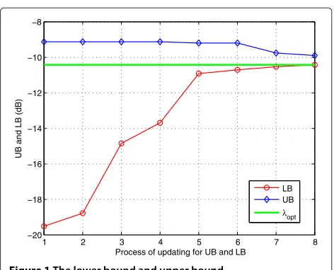
Remark 4. In the process of searching, the lower bound and upper bound are recorded inLBandUB. For a random generated multicast channel withK =32 single-antenna users, we display the process of updating for LB,UB in Figure 1. We can see that the upper bound and lower bound are getting tighter along with the hypothesis tests.
When the gap between LB and UB is less than a given
threshold:UB −LB ≤ δ, we can conclude that the gap
between the best solution we have found and the opti-mal solution to Eq. (12) is no greater thanδ. Ifδ is small, we can early terminate the PASA searching procedure. This scheme, which can be referred to as the truncated PASA, offers a desirable tradeoff between performance and complexity.
3.3 Complexity evaluation of PASA
LetP1,P2,P3denote the probability for case of one bot-tleneck user, case of two botbot-tleneck users, and case of three bottleneck users, respectively. W.l.o.g, we assume
1 2 3 4 5 6 7 8
−20 −18 −16 −14 −12 −10 −8
Process of updating for UB and LB
UB and LB (dB)
LB UB
λopt
Figure 1The lower bound and upper bound.
independent and identically distributed Rayleigh fading between the BS and users. When the BS is equipped with two antennas while all users are single-antenna users, we have derived the bounds forP1,P2,P3.
Theorem 2.For this multicast system, the probability for case of one bottleneck user is P1 = K1; the lower
bound of P2is P2L = 2(KK−21) and the upper bound of P2
is P2U = 16(KK(+K2)−31); consequently, P3 can be bounded as (1−P1−PU2)≤P3≤(1−P1−PL2).
Proof. Please see Appendix 4.
From Theorem 2, we can see that P3 tends to be 1 asK increases. Therefore, the computational complexity of PASA depends only on the third case for asymptoti-cally largeK. Based on this observation, we can obtain a first-order estimation of the computational complexity of PASA.
With knowledge of bounds and form of feasible solu-tion, most of combinations are pruned in PASA. In other words, most of hypothesis tests will be terminated before the division line marked in part III of PASA (Please see Appendix 5). Let Ps denote the probability of
combina-tions which survive after the division line. For a large scale of users, we count the probabilityPsin Table 1. It shows
thatPs≈0 whenKis large. For the hypothesis tests which
are terminated before the division line (with probability close to 1), the complexity involves a constant number of vector multiplications. There are at most CK3 hypothesis tests in the third part of PASA; therefore, the worst-case complexity of PASA isO(K3).
Table 1 Probability of survival combinations
K 8 16 24 32 40 48
Ps 0.0341 0.0226 0.0193 0.0148 0.0147 0.0121
K 56 64 72 80 88 96
Ps 0.0114 0.0103 0.0101 0.0091 0.0086 0.0082
K 104 112 120 128 136 144
Ps 0.0074 0.0071 0.0070 0.0067 0.0065 0.0054
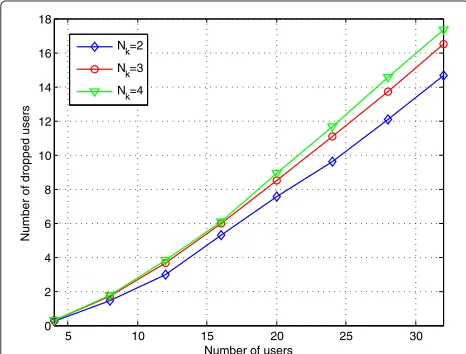
of the hypothesis tests as they cannot be bottleneck users according to Remark 2. Figure 2 shows the average number of dropped users when the users are equipped with multiple antennas. We can see that about half of users can be excluded; therefore, the complexity of PASA is substantially reduced.
4 Iterative two-dimension optimization forM>2
When the base station is equipped with more than two transmit antennas, the max-min fair beamforming prob-lem (5) becomes much more complicated due to the NP-hardness. In this section, an I2DO algorithm is developed for the general case, i.e.,M>2.
4.1 The I2DO algorithm
For a problem that cannot be solved directly, a well-known approach is decomposing it into solvable subproblems. The main idea of I2DO is transforming the problem (5)
into subproblems of M = 2. Considering the
beam-forming vectorwis in the column space of matrix P ∈
CM×2,P∗P=I
2, we can writewas
w=Pu, (36)
whereu =[u1,u2]T,u21+u22 = 1. Substituting Eq. (36) into problem (5), we have an optimization problem with respect tou
5 10 15 20 25 30
0 2 4 6 8 10 12 14 16 18
Number of users
Number of dropped users
Nk=2 Nk=3 Nk=4
Figure 2Average number of dropped users.
max
u∈C2 k=min1,...,K u
∗P∗H∗
kHkP
u
subject to u2=1.
(37)
We can see that Eq. (37) is exactly the max-min fair beamforming problem of two Tx antennas. As showed in Section 3, the optimal solution to Eq. (37) can be obtained efficiently by PASA.
Based on above discussions, an iterative strategy can be adopted to handle the original problem (5). Letwn∈CM,
wn = 1 denote the beamforming vector at then-th
iteration. The beamforming vector at then+1-th step is updated as
wn+1=u1wn+u2vn, u21+u22=1, (38)
wherevn ∈ CM denotes the direction of updating which
is orthogonal town and of unit-length. Note that u1,u2 can be referred to as the complex-valued step size. After definingP =[wn, vn] andu =[u1,u2]T, we can obtain the optimal step size by solving Eq. (37). In other words, we find the optimal beamforming vector on the plane spanned bywnandvn. With this scheme,wn+1always out-performs wn, except that u2 = 0. Hence, the objective function of Eq. (5) is monotonically increasing across iter-ations, and it shall converge to a stationary point. In the iterations, if minkγk(wn+1)−minkγk(wn)is less than a
preset threshold, then the I2DO algorithm can be termi-nated. Here,γk(w) = w∗H∗kHkwdenotes the SNR of the k-th user.
To accelerate the convergence of I2DO, the direction of updating vn should be carefully chosen. Firstly, we
con-sider a rotation fromwn tovn, thus the SNR of thek-th
user can be expressed as a function ofvnand the angle of
rotationθ
γk(θ,vn)=(cosθwn+sinθvn)∗H∗kHk(cosθwn+sinθvn).
After differentiatingγk(θ,vn)with respect toθ, we have
∂γk(θ,vn)
∂θ
θ=0
=2Rew∗nH∗kHkvn
. (39)
If Rew∗nH∗kHkvn
>0, then a tiny rotation fromwnto
vnwill increase the SNR of thek-th user.
LetBn ⊆ {1,· · ·,K}denote the indexes of users whose
SNRs are the lowest at then-th iteration. To improve the SNR of these users, we can rotatewntovnwhich satisfies
Rew∗nH∗kHkvn
>0, ∀k∈Bn,
w∗nvn=0,vn2=1.
(40)
For convenience, we turn it into real-valued form. Construct matricesW∈C2M×2andR∈R2M×(|Bn|)as
W=
Re{wT
n} Im{wTn}
−Im{wTn} Re{wTn} T
where
rk=
Re{H∗kHkwn}
Im{H∗kHkwn}
.
With above definitions and Eq. (40), we have
RT WT
Re{˜vn}
Im{˜vn}
=
1|Bn|
02
, (41)
where the vectorv˜nis a length-relaxed version ofvn. Note
that we choose Re{w∗nH∗kHkv˜n} =1,∀k∈ Bn, w.l.o.g. It is
clear that Eq. (41) are linear equations. Therefore, if|Bn| ≤
2M−2,v˜ncan be obtained by pseudo-inverse, while the
unit-length vectorvnisvn = ˜vn/˜vn. With this scheme,
the convergence rate of I2DO is satisfactory.
In summary, the full procedure of the I2DO algorithm is summarized in Algorithm 1.
Algorithm 1:The I2DO algorithm
1 Initiate vectorw0, threshold,n=0;
2 while|| ≥do
3 choose setBn;
4 construct vectorvnby Eq. (41) and normalization;
5 P=[wn,vn]; calculateuin Eq. (37);
6 wn+1=Pu;
7 =minkγk(wn+1)−minkγk(wn);
8 n=n+1;
9 end
Remark 5.In general, there is no need to choose the step size (u1,u2) optimally [3,8]. Suboptimal algorithms such as the truncated PASA can be used here to obtain an approximate step size in Eq. (37).
4.2 Initialization of I2DO
In the iterations of I2DO, the minimum SNR is non-decreasing, and it will converge to a stable point. How-ever, I2DO is not guaranteed to find the globally optimal beamformer, and it may get trapped into a local opti-mum. As a result, proper initialization of I2DO is of great significance [9].
In [11], Lozano’s alternating gradient method is pro-posed which is quite simple and easily for implementation. It is further improved by choosing Lopez’s initializa-tion and adaptive step size in [12]. Hence, this modified Lozano’s algorithm is called damped Lozano with Lopez’s initialization (dLLI). Considering its low complexity and feasibility, dLLI can be employed to yield initialization points for I2DO. In order to obtain good performance,
dLLI can be executed M times in parallel. Similar to
Lopez’s initialization, the M eigenvectors of kH∗kHk
can be used as the initialization points of dLLI. For each
eigenvector ofkH∗kHk, we invoke dLLI and obtain an
improved vectorwˆm. Finally, the best one is simply chosen
to be the initialization point of I2DO
w0=arg max
ˆ
wm
min
k wˆ
∗
mH∗kHkwˆm. (42)
4.3 Implementation complexity of I2DO
The I2DO algorithm is comprised of the I2DO iterations and computation of initialization vector which requires calling dLLI M times. Let J1,J2 denote the numbers of iterations in I2DO and dLLI. The worst-case computa-tional complexity of the I2DO iterations isO(J1K3), while the complexity involved in the generation of initialization vector isO(J2KM2). So the entire complexity of I2DO is O(J1K3 + J2KM2). It is worthy to note that the actual complexity of I2DO can be further reduced if the trun-cated PASA is used instead of PASA. The worst-case complexity of the SDR-based scheme isO((K+M2)3.5), excluding the additional process of randomization [2]. The overall complexity of the GS-DL method proposed in [4] isO(K(M3+IKM)), whereI denotes the number of iterations in local refinement. Therefore, the SDR-based scheme is less efficient than I2DO and GS-DL.
5 Simulation results
In this section, simulation results are presented to demon-strate the effectiveness of the proposed approaches: PASA and I2DO. The following results are based on 2, 000 Monte-Carlo trials, where independent and identically distributed Rayleigh fading channels between the base sta-tion and users are assumed. Besides, the transmit power is set asP=1.
5.1 Performance of PASA
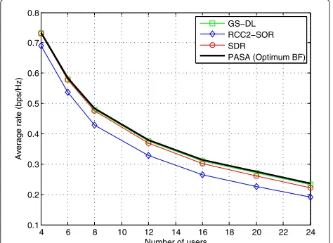
We consider that the base station is equipped with two transmit antennas and all users are single-antenna users, i.e., Nk = 1,∀k, since the GS-DL technique in [4] and
the RCC2-SOR method proposed in [3] cannot han-dle the case of multi-antenna users. Figure 3 displays the achievable rates of different approaches with respect to the number of users. In the SDR-based scheme, the CVX [13] is used to solve the semidefinite program-ming problem. In the subsequent process of random-ization, three randomization techniques: RandA, RandB, and RandC are used to generate 300 candidate vectors where 100 vectors are generated for each (see also [2]). We can see that both the SDR-based scheme and GS-DL perform quite close to PASA which yields the optimal beamformer. While for the RCC2-SOR method, it has about 0.05 bps/Hz performance loss compared to PASA.
4 6 8 10 12 14 16 18 20 22 24 0.1
0.2 0.3 0.4 0.5 0.6 0.7 0.8
Number of users
Average rate (bps/Hz)
GS−DL RCC2−SOR SDR
PASA (Optimum BF)
Figure 3Average achievable rate versus number of users.
distribution function (CDF). It is showed that the SNR loss of the SDR-based scheme and GS-DL are more than 1.5 dB in the worst case, even though their average achievable rates are close to the optimal value.
Figure 5 gives a comparison of average runtime for dif-ferent approaches, where all of them are implemented based on MATLAB. When the number of users is rela-tively small, for instance,K ≤12, the average runtime of PASA is less than those of the other three methods, and therefore, PASA is computationally more efficient. For the
case of K > 12, RCC2-SOR is computationally faster
than PASA; however, it is a suboptimal algorithm and may suffer from severe performance loss.
5.2 Performance of I2DO
Figure 6 shows the average rates achieved by the I2DO
algorithm, the SDR-based scheme and GS-DL forM=8.
−0.50 0 0.5 1 1.5 2 2.5 3 0.1
0.2 0.3 0.4 0.5 0.6 0.7 0.8 0.9 1
SNR loss compared to PASA (dB)
CDF
M=2, K=16, Nk=1
GS−DL SDR
Figure 4SNR loss of the existing algorithms compared to PASA.
4 6 8 10 12 14 16 18 20 22 24 0
0.1 0.2 0.3 0.4 0.5 0.6 0.7
Number of users
Average runtime of Matlab code (sec)
GS−DL RCC2−SOR SDR PASA
Figure 5Average runtime of Matlab codes.
For the SDR-based scheme, 3, 000 candidate vectors are generated by randomization, and the best one is cho-sen as an approximate solution. In the I2DO algorithm,
numbers of iterations in I2DO and dLLI are J1 = 20,
J2 = 100, respectively. When all users are equipped
with single antenna (Nk = 1), both I2DO and GS-DL
have superior performance over the SDR-based scheme, and the gap between them is more than 0.25 bps/Hz
forK ≥ 16. Moreover, I2DO also outperforms GS-DL
especially when the number of users is large. In multiple-antenna user scenario (Nk = 2), GS-DL is not applicable
anymore. Hence, we only compare the performance of I2DO and the SDR-based scheme. Similarly, we can see that I2DO has about 0.3 bps/Hz improvement over the latter.
In the following scenario, the number of users is set asK = 36, where all of them are single-antenna users. The average achievable rates of different methods are
10 15 20 25 30 35 40 45 50 55 60 0.2
0.4 0.6 0.8
1
1.2 1.4 1.6 1.8
2
2.2
Number of users
Average rate (bps/Hz)
GS−DL SDR I2DO Nk=2
Nk=1
compared in Figure 7. Note that 30MK candidate vectors are generated in the randomization process of SDR, since the dimensionality of beamforming problem gets larger as the number of transmit antennas increases [2]. Here, the multicast capacity is achieved by a multi-rank pre-coder [14]. Obviously, the multicast capacity is an upper bound of all achievable rates. From Figure 7, we can see that I2DO is superior to the SDR-based scheme and GS-DL. Moreover, the beamformer designed by I2DO can achieve a large majority of the multicast capacity, while the complexity of encoding and decoding is significantly reduced.
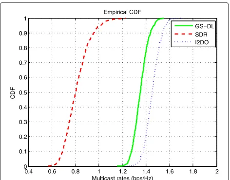
We further provide a detailed comparison for the
sce-nario of M = 24,K = 36,Nk = 1. The cumulative
distribution functions of the multicast rate achieved by above three methods are displayed in Figure 8. Again, I2DO has the best performance and it can achieve almost twice the multicast rate of the SDR-based scheme. As shown in [15], the approximation accuracy of semidefinite relaxation is a decreasing function of the number of users. In other words, the performance of the SDR-based scheme degrades when the number of users increases.
6 Conclusions
For the well-known max-min fair beamforming prob-lem, two efficient algorithms, PASA and I2DO, are pro-posed to handle the case of two Tx antennas and the general case of more than two Tx antennas, respec-tively. In the two-antenna case, PASA is guaranteed to obtain a globally optimal beamformer with worst-case complexity O(K3). While in the general cases, I2DO can decompose the original beamforming prob-lem into a series of two-antenna subprobprob-lems and iter-atively improve the solution by PASA. The superior performance of the proposed algorithms is demonstrated
10 15 20 25 30 35
0.4 0.6 0.8 1 1.2 1.4 1.6 1.8 2
Number of transmit antennas
Average rate of multicast channel (bps/Hz)
Multicast capacity GS−DL SDR I2DO
Figure 7Average rate versus number of transmit antennas.
0.4 0.6 0.8 1 1.2 1.4 1.6 1.8 2 0
0.1 0.2 0.3 0.4 0.5 0.6 0.7 0.8 0.9 1
Multicast rates (bps/Hz)
CDF
Empirical CDF
GS−DL SDR I2DO
Figure 8Cumulative distribution function of the multicast rate.
by comparing them with the state-of-the-art multicasting schemes.
Endnotes
aIf n
k is colored noise and the covariance matrix is
known, it can be pre-whitened at the receiver side. bThe formulaw∗H∗
kHkwin Eq. (3) can be interpreted as
the received SNR of thek-th user. cIt also means that every three of{g
k}Kk=1 are linearly independent.
dThe detailed process of computing these solutions is
demonstrated in the following three cases of bottleneck users.
eThere are some slight modifications in part II of PASA
and the division line marked in part III of PASA is to be used for the complexity analysis.
Appendices
Appendix 1 Proof ofLemma3
In the case of one bottleneck user, w.l.o.g, we assume the
i-th user is the bottleneck user. Hence, we haveγi(x) < γl(x),l∈ {1,· · ·,K}\{i}, whereγi(x)=hi+gTixis the SNR
of the i-th user. To maximize the SNR of the bottleneck user, the optimal solution to Eq. (12) must bex=gi/gi
according to the Cauchy-Schwarz inequality. Besides, it yields an upper bound ofλopt:λopt≤hi+gibyLemma2.
There areKpossible cases of the bottleneck user, so we obtainKupper bounds ofλopt:hk+ gk,k = 1,. . .,K.
We can see that only the index corresponding to the low-est upper bound is possible to be the bottleneck user. Therefore, instead of exhausting K hypothesis tests, we need only to verify if useri = arg mink hk+ gkis the
bottleneck user.
Appendix 2 Proof ofLemma4
In the case of two bottleneck users, w.l.o.g, we assume thei-th andj-th users are the bottleneck users. Then, we haveγi(x) = γj(x) < γl(x),l ∈ {1,· · ·,K}\{i,j}, where
γi(x) = hi +gTixandγj(x) = hj+gTj xdenote SNRs of
thei-th andj-th users, respectively. According to the FJ necessary conditions, an optimal solution to Eq. (12) must have form asx = αgi +βgj, whereα,β have the same
From geometrical perspective, we can see that the opti-mal solution to Eq. (43) must be a vector which is in the cone generated bygiandgj.
Assumingvis an arbitrary unit-length vector which is orthogonal tox, we define a rotation fromxtov
γl(θ )=hl+gTl (xcosθ+vsinθ ), l=i,j. (44)
can be divided in two cases:
case 1 : ξi>0,ξj<0 orξi<0,ξj>0;
case 2 : ξi=ξj=0.
For case 1, it is impossible to improve the solutionxas the rotation always decreases the SNR of bottleneck users. For case 2, we need to consider the second derivative of γi(θ ),γj(θ )with respect toθ
Consider the weighted sum of the second derivative
ασi+βσj= −
θand rotatingxtovwill decrease the SNR of thei-th user. Therefore, it is impossible to improve the solutionxby rotating tov.
From analysis of both cases, we can see that solution x = αgi+βgj,α > 0,β > 0 is the optimal solution to
Eq. (43). According toLemma2, we know the correspond-ing SNRλ = hi +gTi x = hj+gTjxis an upper bound
ofλopt. Ifλ < UB, thenλis a tighter upper bound and we can updateUB =λ. Besides, if the solutionxsatisfies
hk+gTkx≥λ,k=1,. . .,K, then fromLemma2, it is also
an optimal solution to Eq. (12).
Appendix 3 Proof ofLemma5
In case of three bottleneck users, w.l.o.g, we assume the
i-th user, j-th user, and k-th user are the bottleneck users. That is, γi(x) = γj(x) = γk(x) < γl(x),l ∈
{1,. . .,K}\{i,j,k}. According to the FJ necessary condi-tions, an optimal solution to Eq. (12) must have form as x=αgi+βgj+γgk, whereα,β,γ have the same sign. In
particular, ifα >0,β >0,γ >0, thenx=αgi+βgj+γgk
is the optimum solution to problem
max
x∈R3,λ λ
s.t. hl+gTl x≥λ, l=i,j,k
x =1.
(47)
From geometrical perspective, it is easy to see that the optimal solution to Eq. (47) must be a vector in the cone generated bygi,gj, andgk.
Defining vas an arbitrary unit-length vector which is orthogonal tox, we consider the rotation fromxtovand obtainγi(θ ),γj(θ ),γk(θ )as defined in Eq. (44). Taking the first derivative of them with respect toθ, we have
Then,vandxcan be denoted as
are linearly independent. Consequently, at least one of ξi,ξj,ξk is negative, and it is impossible to improve one
of the SNRs without reducing another one. Now, we con-clude that solutionx= αgi+βgj+γgk,α > 0,β > 0,
γ >0 is the optimal solution to Eq. (47).
According toLemma2, the corresponding SNRλ=hi+
gTi x = hj+gTj x = hk +gTkxis an upper bound ofλopt which is the optimal solution of the original problem (12). Ifλ < UB, then we obtain a tighter upper boundUB= λ. Also, if this solutionxsatisfieshk+gTkx≥λ,∀k, then it is
an optimal solution to Eq. (12) byLemma2.
Appendix 4 Proof ofTheorem2
When all users are single-antenna users, the channels can be denoted by
Hk =h∗k, k=1,. . .,K,
where hk ∈ C2. In one bottleneck user case, w.l.o.g, we
assume thei-th user is the bottleneck user. Then, the opti-mal beamforming vector should bewopt =hi/hi[3,5].
Hence, the SNR of the i-th user is γi = hi2 which is a chi-squared distributed random variable with four degrees of freedom [16], while the SNRs of other users are γl = |h∗lwopt|2,l ∈ {1,. . .,K}\{i}. Since the beamform-ing vectorwoptis of unit length and is independent ofhl;
therefore,h∗lwoptis a complex Gaussian variable with zero mean and unit variance. Consequently,γlis a chi-squared distributed random variable with two degrees of freedom. The probability density functions (pdf ) ofγi,γlare given
by [16]
fγi(x)=xe−x fγl(x)=e
−x, l∈ {1,. . .,K}\{i}.
Finally, the probability of one bottleneck user caseP1can be calculated by
In two bottleneck user case, we assume that the i-th and j-th users are bottleneck users. Let γij denote the
SNR of bottleneck users andγl,l∈ {1,. . .,K}\{i,j}denote the SNRs of other users. Similarly, the probability of two bottleneck user caseP2can be expressed as
P2=
i,j
P(γij<min
l=i,jγl). (49)
To calculateP2, firstly we have to derive the closed form ofγijand analyze its pdf.
Assuminghi < hj, then from the fact that both of
them are bottleneck users, we have (see also [5])
hj2>hi2>|h∗ihj|2/hi2. (50)
DefineHijas
Hij=[hi,hj]∈C2×2,
and consider the QR decomposition ofHij
Hij=QR, Q=[q1,q2] , R= As proved in [5], the optimal beamforming vector should be on the plane spanned byhiandhj, sowoptcan
be expressed as the linear combination ofq1,q2
wopt=cosθq1+sinθejφq2, θ ∈[0, π
2), φ∈[0, 2π ). (53)
Noting that the SNRs of bottleneck users are equal, we have
|h∗iwopt|2= |h∗jwopt|2.
Combining it with Eqs. (51) and (53), we obtain
r112 cos2θ = |r∗12cosθ +r22sinθejφ|2. (54)
To maximize the SNRs,φmust be
φ= −∠r12.
Hence, Eq. (54) turns to
r11cosθ = |r12|cosθ+r22sinθ
Finally, the SNR of bottleneck users can be expressed as
γij= r
2 11r222 (r11− |r12|)2+r222
However, it is too complicate to derive the pdf ofγij
due to its complex expression. Instead of computing the precise expression ofP2, we try to provide the bounds of
P2. From the expression ofγij, we can see thatγij ≤ r112. Moreover, with Eq. (52), we have
γij≥
With above results,P2can be bounded as
P2, respectively.
As mentioned before, the beamforming vectorwopt is
only determined by the channels of bottleneck users and hence is independent ofhl,l = i,j. Therefore, the SNRs
of other users γl = |h∗lwopt|2 still follow chi-squared distribution with two degrees of freedom and its pdf is
fγl(x)=e
−x, l∈ {1,. . .,K}\{i,j}.
To derive the lower bound and upper bound ofP2, we turn to analyze the pdf ofr112 = hi2. Letυ denote the
squared normalized inner product ofhiandhj
υ = |h
∗
ihj|2
hi2hj2
, υ∈[ 0, 1] .
Then, Eq. (50) can also be expressed as
hi2<hj2< hi
2
υ .
Noting thatυfollows uniform distribution [17,18], that is,
f(υ)=1, υ∈[0, 1] .
Hence, the cumulative distribution function (cdf ) of hi2is
where factor 2 before the integral denotes that there are two possible case of orders. After differentiation, we obtain the pdf ofr112 in the following
fr2
11(x)=2x
2e−2x.
Consequently, the pdf ofr211
2 is
fr112
2
(x)=16x2e−4x.
Now, the upper bound and lower bound of P2 can be
calculated by
P3 = 1. From above results, it is straightforward to
get the bounds corresponding to the probability of three bottleneck user case
PL3≤P3≤PU3,
wherePL3=1−P1−P2U,PU3 =1−P1−PL2are the lower bound and upper bound ofP3, respectively.
Appendix 5 The Pseudo MatlabTMCode of PASA PART I of PASA: Check ifL=1
%by Lemma 2, a globally optimal solution %has been found
identify i (or j) as the stronger user; S=S\ {i}(orS\ {j});%by Remark 2
continue; %try another pair
%by FJ conditions,
%it is not a valid candidate
continue; end
x=αgi+βgj;
snr=min1≤l≤K (hl+gTl x);
if λ≤snr&(α >0 &β >0)
%by Lemma 4, a globally optimal %solution has been found
return xopt=x, λopt=λ; elseif λ >snr&(α >0 &β >0)
%by Lemma 4, we obtain a tighter %upper bound
UB=λ;
elseif λ≤snr&(α <0 &β <0) %xLB can potentially be an %optimal solution
LB=λ; xLB=x;
elseif λ >snr&(α <0 &β <0)
LB=max(LB,snr);%update the lower bound
end end %for λ end %for (i,j)
PART III of PASA: Check ifL=3
for user combination (i,j,k) drawn from S computea,b,cfrom Eq. (33);
if b2−ac<0
%(i,j,k) is not a valid combination, %go on to try another combination
continue; end
forλ= !
b−√b2−ac
a ,b+
√
b2−ac
a
"
∩[LB,UB]
computeα,β,γ fromEq. (35); if α,β,γ have different signs
%by FJ conditions,
%it is not a valid candidate
continue; end
− − − − − − − − − −division line− − − − − − − −−
x=αgi+βgj+γgk;
snr=min1≤l≤K (hl+gTl x);
if λ≤snr&(α >0 &β >0 &γ >0)
%by Lemma 5, a globally optimal %solution has been found
return xopt=x, λopt=λ;
elseif λ >snr&(α >0 &β >0 &γ >0) %by Lemma 5, we obtain a tighter %upper bound
UB=λ;
elseif λ≤snr&(α <0 &β <0 &γ <0) %xLB can potentially be an %optimal solution
LB=λ; xLB=x;
elseif λ >snr&(α <0 &β <0 &γ <0)
LB=max(LB,snr);%update the lower bound
end end %for λ end %for (i,j,k)
return xopt=xLB, λopt=LB;
Endnotes aIfn
kis colored noise and the covariance matrix is
known, it can be pre-whitened at the receiver side.
bThe formulaw∗H∗
kHkwin (3) can be interpreted as
the received SNR of thek-th user.
cIt also means that every three of{g
k}Kk=1are linearly independent.
dThe detailed process of computing these solutions is
demonstrated in the following three cases of bottleneck users.
eThere are some slight modifications in part II of PASA
and the division line marked in part III of PASA is to used for the complexity analysis.
Competing interests
The authors declare that they have no competing interests.
Acknowledgments
This work was supported by the National Natural Science Foundation of China under grant number 61071094, the National Science and Technology Special Projects of China under grant number 2012ZX03001007-002, and grant number 2012AA01A502 from the National High Technology Research and Development Program of China (863 Program). Parts of this work were presented at the IEEE International Conference on Communications, Ottawa, Ontario, Canada, June 2012.
Author details
1Department of Electronic Engineering and Information Science, University of Science and Technology of China, Hefei, Anhui 230027, China.2Silvus Technologies, Inc, San Diego, CA 92127, USA.
Received: 15 January 2013 Accepted: 17 June 2013 Published: 25 June 2013
References
1. MJ Lopez, Multiplexing, scheduling, and multicasting strategies for antenna arrays in wireless networks, PhD thesis, Dept. of Elect. Eng. and Comp. Sci., MIT. 2002
2. ND Sidiropoulos, TN Davidson, ZQ Luo, Transmit beamforming for physical-layer multicasting. IEEE Trans. Signal Process.54(6), 2239–2251 (2006)
3. R Hunger, DA Schmidt, M Joham, A Schwing, W Utschick, inProc. IEEE ICC. Design of single-group multicasting-beamformers, (Glasgow, June 2007), pp. 2499–2505
4. A Abdelkader, AB Gershman, ND Sidiropoulos, Multiple-antenna multicasting using channel orthogonalization and local refinement. IEEE Trans.Signal Process.58(7), 3922—3927 (2010)
5. II Han Kim, DJ Love, SeungYoung Park, Optimal and successive approaches to signal design for multiple antenna physical layer multicasting. IEEE Trans. Commun.59(8), 2316–2327 (2011)
6. E Song, Q Shi, M Sanjabi, R Sun, Robust SINR-constrained MISO downlink beamforming: when is semidefinite programming relaxation tight? EURASIP J. Wirel. Commun. Netw.2012(1), 1–11 (2012)
8. GH Golub, CV Loan,Matrix Computations(Johns Hopkins University Press, Baltimore, 1996)
9. S Boyd, L Vandenberghe,Convex Optimization(Cambridge University Press, Cambridge, 2004)
10. MS Bazaraa, HD Sherali, CM Shetty,Nonlinear Programing: Theory and Algorithms. (John Wiley & Sons, Hoboken, 2006)
11. A Lozano, inProc. IEEE Int. Conf. Acoustics, Speech and Signal Processing. Long-term transmit beamforming for wireless multicasting (Honolulu, April 2007), pp. III-417–III-420
12. E Matskani, ND Sidiropoulos, ZQ Luo, L Tassiulas, Efficient batch and adaptive approximation algorithms for joint multicast beamforming and admission Control. IEEE Trans. Signal Process.57(12), 4882–4894 (2009) 13. M Grant, S Boyd, CVX: Matlab software for disciplined convex
programming, version 2.0 beta (2013) http://cvxr.com/cvx. Accessed June 2013
14. N Jindal, ZQ Luo, inProc. IEEE Int. Symp. Inf. Theory. Capacity limits of multiple antenna multicast (Seattle, July 2006), pp. 1841–1845 15. ZQ Luo, WK Ma, AMC So, Y Ye, S Zhang, Semidefininite relaxation of
quadratic optimization problems. IEEE Signal Process. Mag. 27(3), 20–34 (2010)
16. TW Anderson,An Introduction to Multivariate Statistical Analysis(John Wiley & Sons, Hoboken, 2003)
17. CK Au-Yeung, DJ Love, On the performance of random vector
quantization limited feedback beamforming in a MISO system. IEEE Trans. Wirel. Commun.6(2), 458–462 (2007)
18. JD Love, RW Heath, Grassmannian beamforming for multiple-input multiple-output wireless systems. IEEE Trans. Inf. Theory.49(10), 2735–2747 (2003)
doi:10.1186/1687-6180-2013-121
Cite this article as:Duet al.:Optimum beamforming for MIMO multicast-ing.EURASIP Journal on Advances in Signal Processing20132013:121.
Submit your manuscript to a
journal and benefi t from:
7Convenient online submission 7Rigorous peer review
7Immediate publication on acceptance 7Open access: articles freely available online 7High visibility within the fi eld
7Retaining the copyright to your article