Dynamic rupture simulation of the 2011 off the Pacific coast of Tohoku
Earthquake: Multi-event generation within dozens of seconds
Hiroyuki Goto1, Yojiro Yamamoto2, and Saeko Kita3
1Kyoto University, Gokasho, Uji, Kyoto 611-0011, Japan
2Japan Agency for Marine-Earth Science and Technology, 3173-25 Showa-machi, Kanazawa-ku, Yokohama 236-0001, Japan 3Tohoku University, 6-6 Aza-Aoba, Aramaki, Aoba-ku, Sendai 980-8579, Japan
(Received December 22, 2011; Revised June 4, 2012; Accepted June 12, 2012; Online published January 28, 2013)
We focus on a complex rupture process, namely, multi-event generation within about 50 seconds during the 2011 off the Pacific coast of Tohoku Earthquake (Mw9.0). We perform a 2D dynamic rupture simulation in
order to explain physically the rupture process along the cross-section passing through the hypocenter. Realistic velocity structures are introduced into the simulation model. The dynamic parameters are selected by referring to kinematic source inversion results. The first significant event is generated on the deeper side of the fault. The scattered waves, mainly from the free surface, generate a stick-slip around the hypocenter, and then a second significant event is triggered. The synthetic waveforms consist of two major wave groups that are consistent with the observed ground motions.
Key words: The 2011 off the Pacific coast of Tohoku Earthquake, dynamic rupture simulation, strong ground motion.
1.
Introduction
On March 11, 2011, at 14:46 (JST, GMT+9), the off the Pacific coast of Tohoku Earthquake (Mw9.0) hit the eastern
part of mainland Japan; the earthquake and, in particular, the great tsunami that followed resulted in the death of more than ten thousand people. Strong ground motions during the earthquake were observed over almost the whole region of Japan by K-NET, KiK-net organized by the National Re-search Institute for Earth Science and Disaster Prevention (Aoiet al., 2011), and by other seismic networks. At least 18 stations observed over 9.8 m/s2 of peak ground
acceler-ations in horizontal components, and two stacceler-ations observed a seismic intensity over 6.5 on the Japan Meteorological Agency scale.
Several research groups have reported the source rupture process during the earthquake. GPS data and low-frequency ground motions imply that a large slip region is located on the shallower side of the seismic fault (Miyazakiet al., 2011; Yoshida et al., 2011). On the other hand, ground motions band-passed within about 0.1–5 Hz imply that sev-eral strong motion generation areas (SMGAs) are located on the deeper side of the seismic fault (Kurahashi and Irikura, 2011; Asano and Iwata, 2012), and the high-frequency ra-diation area, higher than about 0.5 Hz, is also estimated, by the back-projection method, to be located on the deeper side (Ishii, 2011; Wang and Mori, 2011; Zhanget al., 2011). This indicates that the locations of seismic wave radiation areas depend on the frequency bands (Koperet al., 2011).
Copyright cThe Society of Geomagnetism and Earth, Planetary and Space Sci-ences (SGEPSS); The Seismological Society of Japan; The Volcanological Society of Japan; The Geodetic Society of Japan; The Japanese Society for Planetary Sci-ences; TERRAPUB.
doi:10.5047/eps.2012.06.002
Strong ground motions observed in the Miyagi and Iwate prefectures, close to the epicenter region, consist of two major wave groups with an interval of about 50 s (e.g. Kurahashi and Irikura, 2011; Nakaharaet al., 2011). The origins of the wave groups are estimated to be on the deeper side of the hypocenter, and the origins are located close to each other (Kurahashi and Irikura, 2011; Asano and Iwata, 2012). However, there is a gap of about 50 s between the rupture times of the corresponding events. The important question is what is the physical mechanism that can ex-plain the time lag. Hereafter, the events are referred to as a “multi-event” in a single earthquake (e.g. Kikuchi and Kanamori, 1982; Sawadaet al., 1992).
Duan (2012) has performs 3D spontaneous rupture sim-ulation by considering a subducting seamount just up-dip of the hypocenter. The result shows significant slip near the trench, and the seafloor deformation agrees well with observations (Satoet al., 2011). High-frequency radiations are modeled by three high-strength patches located at the down-dip portion; however, he does not attempt to repro-duce details of the high-frequency radiation feature as com-pared to the actual observed ground motions.
In this study, we carry out a dynamic rupture simulation that models physically consistent slips with stress fields and interface frictions on the fault plane. We especially focus on the numerical modeling of multi-event generation along the dip direction. Ideet al.(2011) have proposed that the major effect can be attributed to a dynamic overshoot due to the fault crossing the free surface, whereas we demonstrate that simulation without the fault crossing the free surface can represent a rupture process consistent with the observed ground motions.
1168 H. GOTOet al.: DYNAMIC RUPTURE SIMULATION OF 2011 TOHOKU EARTHQUAKE
2.
Method
Several kinds of numerical methods have been applied to dynamic rupture simulation, and their accuracies have been discussed via a code validation project (e.g. Harriset al., 2009). Most of the methods are categorized as either domain-based methods (e.g., FDM and FEM), or boundary-based methods (e.g., BIEM). Gotoet al.(2010) proposed an alternative hybrid approach: viz., the boundary-domain method (BDM). In this method, instantaneous traction change is represented by the combination of a direct term calculated by a boundary-based method for a homogeneous full space, and a residual term calculated from the dif-ferences between two solutions for a target heterogene-ity model and for a homogeneous full space model by a domain-based method. BDM guarantees accuracy of the stress field close to the fault plane and its applicability to heterogeneous structures.
However, BDM is not applicable to problems with strong heterogeneities beside the fault plane, e.g. faults crossing the material interfaces and faults located on the interfaces of different materials. Actual seismic faults, including the subduction fault corresponding to the earthquake, fall under these conditions. On the other hand, domain-based methods are applicable to model the strong heterogeneities, whereas much denser grids and/or finer meshes than the usual wave propagation problems are required to ensure the accurate and stable simulation of the dynamic ruptures (e.g. Dayet al., 2005). Also, special approaches are required to repre-sent the time-dependent dislocations on the fault plane, such as the split-node technique (e.g. Oglesby and Archuleta, 2000; Dalguer and Day, 2007; Kanekoet al., 2011), and it is difficult to embed a low-angle dipping fault with such approaches. This is because a modification of the local co-ordinate system for FDM (e.g. Kase and Day, 2006) does not simulate well the low-angle case, and a mesh with a high aspect ratio and/or a triangular mesh for FEM give a worse accuracy (e.g. Yoshida, 2010). This means that the domain-based methods for a low-angle dipping fault remain a problem, and they also require great calculation costs to identify an appropriate parameter set for spontaneous rup-ture simulation.
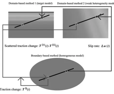
BIEM for a homogeneous medium has been applied to historical earthquakes to discuss physical properties (e.g. Aochi and Fukuyama, 2002; Fukuyamaet al., 2009). The calculation does not exactly follow the actual heterogeneity structures, although some important features have been re-vealed. Here, we apply BIEM for a homogeneous medium to a spontaneous rupture simulation, and also consider addi-tional terms originating from the heterogeneity by introduc-ing the concept of BDM, namely pseudo-BDM (pBDM). As in the case of BDM, we carry out the following three calculations in parallel: (B) a boundary-based method for a homogeneous full space, (D1) a domain-based method for the target model that we want to simulate, and (D2) a domain-based method for a weak heterogeneity model rep-resented by a layered structure, as shown in Fig. 1. To cre-ate the third model, the physical parameters of the fault are homogeneously extended along the normal direction of the fault.
LetTB,TD1, andTD2be the traction changes calculated
Fig. 1. Calculation procedure of pseudo-BDM (pBDM). pBDM requires three parallel calculations: (1) a boundary-based method for a homo-geneous full space (bottom), (2) a domain-based method for the target model (left top), and (3) a domain-based method for a weak hetero-geneity model represented by a layered structure (right top). Color gra-dations in the top figures indicate a conceptual map of material hetero-geneity, such as velocity structures, as shown in Fig. 2. An instanta-neous traction change is represented by the combination of a direct term calculated from the boundary-based method and a residual term calcu-lated from the differences between two solutions of the domain-based methods.
from the boundary-based method and two domain-based methods, respectively. TD1consists of the traction change
due to the direct contribution propagated from the slip re-gion, and also the perturbations due to the heterogeneities, e.g. reflected terms from the material interfaces, and re-fracted terms propagating through the high-velocity zone. On the other hand,TD2consists of the terms directly prop-agated along the fault plane because the fault plane is par-allel to the direction of velocity changes. In order to extract the perturbations fromTD1, it is supposed that the differ-ence betweenTD1andTD2are the perturbations. Then, we
add this toTBin order to include the effects from
hetero-geneity. Although the perturbationTD1−TD2includes the
contribution via reflected and refracted waves, the material properties of D2 are not exactly the same as those of B. If the discrepancy between B and D2 is assumed to be small, e.g., the main part of the rupture is located in an almost ho-mogeneous material, the instantaneous traction changeT is approximated by the combination ofTB,TD1, andTD2, as
follows:
T(t)≈TB(t)+TD1(t)−TD2(t). (1)
The detail scheme in time progress is identical to the BDM introduced by Gotoet al.(2010). In the following section, we show some numerical tests such as the representation of the perturbationTD1−TD2, and the small size of
sponta-neous rupture simulation.
3.
Numerical Model
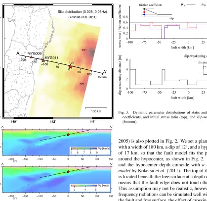
Fig. 2. Geometry of target cross-section (A–A) (top), and velocity mod-els,Vp andVs, on the cross-section (A–A) (Yamamotoet al., 2011)
(bottom). The star denotes the hypocenter of the 2011 off the Pacific coast of Tohoku Earthquake. The circles on the land are the sites record-ing strong ground motions, and the triangles are the locations of K-NET MYG009 and MYG011. Slip distribution estimated by Yoshidaet al.
(2011) is plotted together. The thick line on the cross-section is the fault model, and the dotted lines are the depth of the plate boundary (Itoet al., 2005; Miuraet al., 2005).
passes through the hypocenter estimated by Yamamotoet al.(2011), and the orientation is normal to the strike direc-tion of the seismic fault (N103◦E). The width and depth of the cross-section are 380 km and 90 km, respectively. Two SMGAs estimated by Asano and Iwata (2012) and Kurahashi and Irikura (2011) are located almost on the cross-section. As shown in Fig. 2, the sites observing strong ground motions are distributed across the mainland. Two of them, K-NET MYG009 and MYG011, are located just on the cross-section.
The tomography model by Yamamoto et al. (2011) is applied to the crust velocity structure on the cross-section. Figure 2 also shows the applied velocity model of aP-wave (Vp) and anS-wave (Vs). The plate boundary of the North American and Pacific plates (Itoet al., 2005; Miuraet al.,
Fig. 3. Dynamic parameter distributions of static and dynamic friction coefficients, and initial stress ratio (top), and slip-weakening distance (bottom).
2005) is also plotted in Fig. 2. We set a planar fault model with a width of 180 km, a dip of 12◦, and a hypocenter depth of 17 km, so that the fault model fits the plate boundary around the hypocenter, as shown in Fig. 2. The dip angle and the hypocenter depth coincide with a unified source modelby Koketsuet al.(2011). The top of the fault model is located beneath the free surface at a depth of 367 m. This means that the fault edge does not touch the free surface. This assumption may not be realistic, however if the high-frequency radiations can be simulated well without crossing the fault and free surface, the effect of crossing is not always required to simulate the high-frequency radiation. Also, there are no evidences of high-frequency radiations from the top of the fault (e.g. Koper et al., 2011; Asano and Iwata, 2012). If we focus on the high-frequency radiation, the crossing is of not much significance in the simulation.
The boundary integral equation method (BIEM) (Tada and Yamashita, 1997; Gotoet al., 2010) is applied as the boundary-based method, and the finite-difference method (FDM) (Levander, 1988) is applied as the domain-based method in pBDM. The velocity models for BIEM are set to be 7.34 km/s forVpand 4.20 km/s forVs, which are the av-erage values on the deeper side of the fault. Density models for both BIEM and FDM are evaluated from the empirical density-Vprelation of Ludwiget al.(1970), which has been validated by Miuraet al.(2005). The numerical scheme of FDM is of fourth-order accuracy in space, and of second-order accuracy in time using staggered grids. The element size of BIEM is 87.9 m, and the grid intervals of FDM are homogeneously 100 m. The time step intervals of both methods are set at 4.77×10⁻³ s. The Courant-Friedrichs-Lewy conditions for BIEM and FDM are 0.399 and 0.40, respectively. The maximum support frequency of FDM is 1.34 Hz. Internal damping of the crust structure is set to be
Q =100f and installed by using the approach of Graves (1996).
1170 H. GOTOet al.: DYNAMIC RUPTURE SIMULATION OF 2011 TOHOKU EARTHQUAKE
Fig. 4. Characteristics of perturbation terms calculated from the differ-ences between solutions from the target model (D1) and the layered model (D2); velocities in normal component and shear traction changes observed along the fault plane (top). A double-couple point source is located at−58 km along the fault width. Seismic ray traces ofS-wave for D1,S, and for D2, (S) (bottom).
friction law (Ida, 1972), and the rate-dependency of friction is not considered. In such a case, the dynamic parameters consist of the initial stress ratio μ0, static and dynamic
friction coefficientsμp,μr, and the slip-weakening distance DC. The stress ratio is defined by dividing the initial shear traction by the normal stress. When the shear traction is unloaded, the value of the last friction strength is stored. After the traction reaches the friction strength again, the slip is allowed. This assumption is consistent with a standard elasto-plastic constitutive model.
Figure 3 shows the distributions of the dynamic parame-ters, which are evaluated by trial and error in order to rep-resent the location of SMGAs by Asano and Iwata (2012), whilea prioriinformation about the plate couplings and the inflections is not considered. The origin of the axis along the fault coincides with the hypocenter. A constant value of static friction, 0.6, is assumed over the fault. A 3-km-wide nucleation zone is located around the hypocenter from−1.5 to 1.5 km, where the initial stress ratio, μ0 = 0.60625,
slightly exceeds the static friction coefficient, μp = 0.6.
The stress condition allows the rupture to start from the nu-cleation zone (e.g. Fukuyama and Madariaga, 1998). Two high stress drops are assumed in the deeper region: (1) from
−65 to−45 km, and (2) from−35 to−15 km. The for-mer region assumes μr = 0.35, μ0 = 0.475 ∼ 0.598,
andDC = 0.8 m. The latter region assumesμr = 0.475,
μ0=0.506∼0.538, andDC =1.6 m. The barrier region,
with a 5-km width located from−45 to−40 km, does not
Fig. 5. Comparison of slip-rate time histories calculated by pBDM and FEM. The mesh size of FEM is set to be 50 m (left), and 25 m (right).
allow slip. Regions with negative stress drops and a large slip-weakening distance are located at the bottom of the fault in order to represent a ductile rupture and a yielding of the surrounding materials (Aochi and Fukuyama, 2002). The dynamic friction increases in the shallower region in order to reduce the slip-rate amplitudes (Wada and Goto, 2012), because the stopping front from the shallower edge is assumed to be less dominant in this simulation. This as-sumption is consistent with the hypothesis that the effect of crossing the fault to free surface is not significant in gen-erating high-frequency radiation. Uniform distribution of the normal stress, 160 MPa, is assumed, and normal stress changes due to the rupture are considered in this simulation. In order to check the performance of pBDM to the ve-locity model, we show the results of two simple tests; (1) to see the perturbation waves under the excitation from a double-couple point source, and (2) to see the rupture prop-agations. First, we examined the point source problem. The double-couple source is located at−58 km along the fault width, the seismic moment per unit length is 4.74 GN, the arms of the moment correspond to the fault dip angle, and smoothed ramp function with 1.0 Hz of the center frequency is adopted to the source time function. Figure 4 shows the calculated velocities in the normal component to the fault, and the calculated shear traction changes on the fault plane.
vD1andTD1 are calculated from the model D1, the target
model, andvD2andTD2are from D2, the layered model.
The perturbationsvD1−vD2andTD1−TD2around the point
source from−70 to−46 km are smaller thanvD1andTD1
themselves. ForTD1, additional phases are observed around 20–25 s, andTD1−TD2extracts the phases considered to be the effect from the heterogeneity. From−22 to−6 km, the arrival time of the main phase ofvD1is faster thanvD2, and causes the amplitude of perturbations to increase. Since re-fracted waves for model D2 are not observed along the fault plane, the faster phase corresponds to the refracted waves considered to be the contribution from the velocity hetero-geneity. Figure 4 also shows the seismic ray traces of the
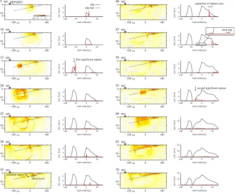
re-Fig. 6. Snap shots of velocity wave fields and slip and slip-rate distributions on the fault plane. At each time step, the color maps show the absolute values of particle velocity (left column). The black and red lines show the distribution of slip and slip-rate, respectively (right column).
spectively, and travel times, 13.15 s and 14.12 s at−6 km, are also marked on the velocity and traction change. The differences of ray traces and travel times indicate that the perturbations contain the refraction waves, and the travel times of the perturbations are well calculated. Therefore, we assume that we are able to discuss the time gaps due to the perturbations based on the results of pBDM.
We also perform another rupture simulation for a trimmed area of 30×50 km2from the velocity model. We
focus on the area around the first high stress drop region. A fault model with a width of 24 km trimmed from the orig-inal model is adopted, and a 3-km-wide nucleation zone is set to be around −58 km along the fault width. The dy-namic parameters are set to beμp =0.6,μr = 0.35 and DC =0.8 m over the whole fault plane, andμ0=0.60625
in the nucleation zone andμ0 = 0.41875 in the other
re-gion. The velocity and density models are the same as with the simulation model. For the reference solutions, a finite-element method (FEM) with split nodes on the fault plane is applied (e.g. Oglesby and Archuleta, 2000). Two different sizes of mesh layout are adapted to the fault, and the mesh sizes are, on average, 50 m and 25 m, respectively. Figure 5 shows the slip-rate time histories calculated by pBDM and
FEM. The synthetic slip-rates from pBDM agrees well with the FEM results, even though pBDM uses coarser grid in-tervals than the size of the FEM mesh. This supports the applicability of pBDM, at least in the deeper side of the fault model.
4.
Results and Discussions
Figure 6 shows snapshots of the absolute values of the simulated particle velocities, and slip and slip-rate distribu-tions, on the fault plane, and Fig. 7 shows a comparison of initial and final shear tractions. Rupture is initiated at the hypocenter within 10 s. Seismic waves propagate in the deeper and shallower directions of the fault width, and then the first significant event is triggered at around−60 km after about 15 s. The event generates seismic waves of large am-plitude in the shallower direction. The seismic waves con-sist of a direct wave propagating along the fault plane and scattered waves mainly reflecting on the free surface. When the direct waves reach the vicinity of the hypocenter where slips have occurred in the initial stage, the slips are excited again within 25–35 s. The direct waves also expand the rup-ture area to the shallower region in about 35–55 s. Ideet al.
oc-1172 H. GOTOet al.: DYNAMIC RUPTURE SIMULATION OF 2011 TOHOKU EARTHQUAKE
Fig. 7. Comparison of initial and final shear tractions. The differences indicate the stress drop of the simulation.
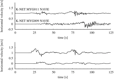
Fig. 8. Observed velocity waveforms at K-NET MYG011 and MYG009 (top), and the corresponding synthetic velocity waveforms (bottom).
curred on the deeper side, and that the rupture propagated toward the shallower side. The simulated rupture process is consistent with Ideet al.(2011).
At the same time, the scattered waves reach the fault plane after 40 s, and generate a stick-slip with low slip-rates around the hypocenter. Here, the stick-slip means that slips in the region repeat the stopping and rupturing. This causes a crack growth gradually expanding the ruptured area in the deeper direction, and then the second significant event is triggered at around−30 km after about 55 s. This event generates seismic waves of large amplitude propagat-ing mainly in the landward direction.
Synthetic velocity waveforms at the location correspond-ing to K-NET MYG011 and MYG009 (see Fig. 2) are com-pared to the observed velocity waveforms at MYG011 and MYG009, as shown in Fig. 8. The observed waveforms are N103◦E components parallel to the cross-section and band-passed within 0.05–1.35 Hz. Notice that the synthetic waveforms are calculated for a 2DP-SVwave field, and the amplitudes and the phases should not be directly compared. The synthetic waveforms show two significant phases with an interval of about 50 s, which is consistent with the ob-served waveforms. The first phase, at about 20–50 s, is generated from the first event, which took place at about
−60 km along the fault at about 15 s. The second phase, at about 65–100 s, is generated from the second event, which took place at about−30 km along the fault at about 55 s. The second phase of both the observed and synthetic waves contains an initial low-frequency stage, at about 65–75 s for MYG011, and a following high-frequency phase. The
Fig. 9. Best fit models of the simulated slip distribution with a superposi-tion of spatial basis funcsuperposi-tions, (1) box-car basis and (2) triangle basis.
time intervals between the first and second phases corre-spond to the interval between the ruptures at about 15 s and 55 s. Within these 40 s, the first 25 s corresponds to the time interval of the scattered waves, and the following 15 s corresponds to the time for crack growth.
The barrier set in the deeper side of the fault may play an important role in the generation of the multi-event. In contrast, no clear barriers are seen in the rupture processes estimated by kinematic source inversions. We suppose that the barrier of our model is consistent with the rupture pro-cesses because the spatial resolutions in the inversions may not be sufficient to reveal it, this has been discussed in the
Source Inversion Validationproject (Pageet al., 2011). For the earthquake, we select four inversion results by Ideet al.
(2011), Miyazakiet al. (2011), Suzukiet al.(2011), and Yoshidaet al.(2011), to compare the maximum spatial res-olutions in their inversion schemes. The slip distributions are represented by the superposition of the basis functions such as the box-car basis (Suzukiet al., 2011; Yoshidaet al., 2011) and the triangle basis (Ideet al., 2011; Miyazaki
et al., 2011). The spatial sizes, e.g. the size of sub-faults (Suzukiet al., 2011; Yoshidaet al., 2011), are usually se-lected such that the dominant frequency caused by the spa-tial periodicity is well outside the frequency range of analy-sis (e.g. Sekiguchiet al., 2000). In addition, the coefficients for each basis are constrained by prior information in the Bayesian approach such as Akaike’s Bayesian Information Criterion (ABIC) (e.g. Ide and Takeo, 1997; Sekiguchiet al., 2000), and the constraint results in the slip distribution being smoothed.
We consider an ideal condition to estimate the slip distri-bution from the slip data obtained just on the fault plane without any observation noises. Figure 9 shows best fit models of the simulated slip distribution with a superpo-sition of spatial basis functions. The spatial sizes of each basis correspond to the parameters of Suzukiet al.(2011), Yoshidaet al.(2011), Miyazakiet al.(2011) and Ideet al.
(2011), respectively. Three of the models cannot estimate the existence of the barrier. One model represented by a triangle basis of 10 km intervals detects no slip region at
−40 km. The model would be obtained if the records ob-tained only on the fault plane were available. However, in the actual situation, smoothing is necessary because of con-straints.
Fig. 10. Comparison of simulation results between the original case and reference case 1 (without free surface); final slip distribution (top) and synthetic velocity waveforms (bottom).
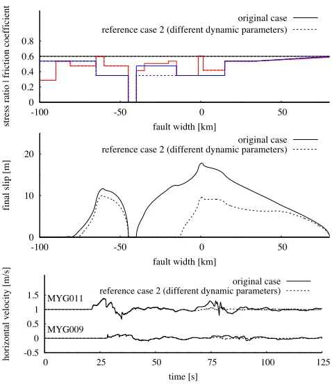
Fig. 11. Comparison of simulation results between the original case and the reference case 2 (different dynamic parameters); friction coefficient (top), final slip distribution (middle) and synthetic velocity waveforms (bottom).
(2012), have estimated the locations of SMGAs. Constant stress drops and square areas of SMGAs are assumed, and the locations, rise time, rupture starting point, and the stress drop are estimated by a trial-and-error approach (Kurahashi and Irikura, 2011), and a grid search (Asano and Iwata, 2012). The procedures infer that a spatial variation within the size of SMGA is averaged. In addition, the relative lo-cations of the two SMGAs are opposite to each other. This implies that the accuracy of SMGA locations is the order of SMGA size. Therefore, it may be difficult to distinguish the barrier based on the results from kinematic source
in-Fig. 12. Comparison of simulation results between the original case and the reference case 3 (another realization); friction coefficient (top), final slip distribution (middle) and synthetic velocity waveforms (bottom).
versions.
In order to clarify the effect of the free surface on the generation of the second significant event, we perform two other reference simulations, case 1: the same dynamic pa-rameters withouta free surface, and case 2: different dy-namic parameterswitha free surface. The velocity model beneath a depth of 0 km is set to be the same model as in the previous simulation, and the model above 0 km for case 1 is equal to the velocities of the uppermost layer of the pre-vious model. The dynamic parameters, fault geometry, and calculation conditions are the same as in the previous simu-lation for case 1, while bothμ0andμrfrom−40 to−20 km
are reduced to 0.35 for case 2.
Figure 10 shows the final slip distribution and velocity waveforms for case 1 compared to the previous results, denoted as the “original case”. Notice that the displayed synthetic waveforms for case 1 are multiplied by a factor of two to account for twice the amplification on the free surface. Final slips for the first significant event at around
−60 km are similar to each other, whereas slips for the second event are insignificant. Likewise, for the second wave group, the final slip distribution is only significant in the model with a free surface. Therefore, the effect of the free surface is essential to the generation of the second events.
signifi-1174 H. GOTOet al.: DYNAMIC RUPTURE SIMULATION OF 2011 TOHOKU EARTHQUAKE
cant event is triggered in the original simulation, the rupture front has just arrived at the shallower fault edge. If the ori-gin of the second wave group is the arrival of the rupture at the free surface, the second wave group would appear in the result for case 2.
The accuracy of the simulated result in the shallower re-gion may not be well guaranteed. Furthermore, the modeled fault does not reach the free surface. These factors result in an underestimation of the final slips in the shallower region compared to the inversion results. However, we point out that a significant effect from the shallower region is not re-quired for the multi-event generation.
Notice that the dynamic parameters are not validated by comparing the amplitudes between observed and synthetic waveforms because the 2DP-SV wave field does not sim-ulate the actual geometric spreading in 3D. The parameter set of our original model is the best we have found, but this may not be the optimum set. Therefore, it is worth showing the justifiability of our choice of parameter set.
In case 3, μp, μr, and DC from −40 km to −20 km
are set to be 0.6, 0.35 and 0.8 m, respectively, which are the same as the values from−65 to−45 km. The model gives the same fracture energy with the original model at the area corresponding to the generation of the second sig-nificant event. The initial stress ratio is modified to con-trol the rupture time at the area. Figure 12 shows the dy-namic parameters, final slip distributions and velocity wave-forms. The area from−40 km to−20 km is ruptured, and it generates the second significant event. As seen in the comparison of the waveforms, the second wave group is clearly observed at the same time as the result for the orig-inal case. The amplitudes of the second wave group are about twice larger than in the original case, because a larger stress drop is assumed. This implies that the absolute val-ues of dynamic parameters for the second significant event cannot be determined quantitatively, and 3D simulations of the dynamic rupture and the seismic wave propagation are required. However, we emphasize that the generation mech-anism of the second significant event is not directly related to the values because of the causality.
5.
Conclusion
We simulate the dynamic rupture process that occurred during the 2011 off the Pacific coast of Tohoku Earthquake on the cross-section passing through the hypocenter. The first significant event occurred at around−60 km along the fault width direction. The waves, scattered mainly from the free surface, come back to the fault plane in about 25 s, and generate a stick-slip with small amplitude around the hypocenter. The stick-slips expand the ruptured area to the deeper side, and then the second significant event is triggered. The synthetic waveforms consist of two major wave groups, which are similar to the observations.
Acknowledgments. We thank two anonymous reviewers and the editor Prof. Takashi Furumura for their thorough comments. We are grateful to the following persons for the useful information they provided us and for helpful discussions: Professor Kazuro Hirahara, Professor Sumio Sawada, Professor Shin’ichi Miyazaki, Dr. Kimiyuki Asano, Dr. Wataru Suzuki, Dr. Hiroe Miyake, and many other researchers. This study was supported in part by
the Grant-in-Aid for Young Scientists B of the Japan Society for the Promotion of Science. We offer our thanks to NIED for the contributions to the strong ground motion observations, namely, K-NET, KiK-net.
References
Aochi, H. and E. Fukuyama, Three-dimensional nonplanar simulation of the 1992 Landers earthquake,J. Geophys. Res.,107, 2039, 2002. Aoi, S., T. Kunugi, W. Suzuki, N. Morikawa, H. Nakamura, N. Pulido,
K. Shiomi, and H. Fujiwara, Strong motion characteristics of the 2011 Tohoku-oki earthquake from K-NET and KiK-net,Proc. of 2011 SSA Annual Meeting, 2011.
Asano, K. and T. Iwata, Source model for strong ground motion generation in the frequency range 0.1–10 Hz during the 2011 Tohoku earthquake,
Earth Planets Space,64, this issue, 1111–1123, 2012.
Dalguer, L. A. and S. M. Day, Staggered-grid split-node method for spon-taneous rupture simulation,J. Geophys. Res.,112, B02302, 2007. Day, S. M., L. A. Dalguer, N. Lapusta, and Y. Liu, Comparison of finite
difference and boundary integral solutions to three-dimensional sponta-neous rupture,J. Geophys. Res.,110, B12307, 2005.
Duan, B., Dynamic rupture of the 2011 Mw9.0 Tohoku-oki earthquake: roles of a possible subducting seamount, J. Geophys. Res., 2012 (in printing).
Fukuyama, E. and R. Madariaga, Rupture dynamics of a planar fault in a 3D elastic medium: rate- and slip-weakening friction,Bull. Seismol. Soc. Am.,88, 1–17, 1998.
Fukuyama, E., R. Ando, C. Hashimoto, S. Aoi, and M. Matsu’ura, A physics-based simulation of the 2003 Tokachi-oki, Japan, earthquake to predict strong ground motions,Bull. Seismol. Soc. Am.,99, 3150–3171, 2009.
Goto, H., L. Ram´ırez-Guzm´an, and J. Bielak, Simulation of spontaneous rupture based on a combined boundary integral equation method and finite element method approach: SH and P-SV cases,Geophys. J. Int., 183, 975–1004, 2010.
Graves, R. W., Simulating seismic wave propagation in 3D elastic me-dia using staggered-grid finite differences,Bull. Seismol. Soc. Am.,86, 1091–1106, 1996.
Harris, R. A., M. Barall, R. Archuleta, E. Dunham, B. Aagaard, J. P. Ampuero, H. Bhat, V. Cruz-Atienza, L. Dalguer, P. Dawson, S. Day, B. Duan, G. Ely, Y. Kaneko, Y. Kase, N. Lapusta, Y. Liu, S. Ma, D. Oglesby, K. Olsen, A. Pitarka, S. Song, and E. Templeton, The SCEC/USGS dynamic earthquake rupture code verification exercise,
Seismol. Res. Lett.,80, 119–126, 2009.
Ida, Y., Cohesive force across the tip of a longitudinal-shear crack and Griffith’s specific surface energy, J. Geophys. Res.,77, 3796–3805, 1972.
Ide, S. and M. Takeo, Determination of constitutive relations of fault slip based on seismic wave analysis,J. Geophys. Res.,102, 27379–27391, 1997.
Ide, S., A. Baltay, and G. C. Beroza, Shallow dynamic overshoot and energetic deep rupture in the 2011 Mw 9.0 Tohoku-Oki earthquake,
Science,332, 1426–1429, 2011.
Ishii, M., High-frequency rupture properties of theMw9.0 off the Pacific coast of Tohoku Earthquake,Earth Planets Space,63, 609–614, 2011. Ito, A., G. Fujie, S. Miura, S. Kodaira, R. Hino, and Y. Kaneda, Bending of
the subducting oceanic plate and its implification for rupture propaga-tion of large interplate earthquake off Miyagi, Japan, in the Japan trench subduction zone,Geophys. Res. Lett.,32, L05310, 2005.
Kaneko, Y., J. P. Ampuero, and N. Lapusta, Spectral-element simulations of long-term fault slip: effect of low-rigidity layers on earthquake-cycle dynamics,J. Geophys. Res.,116, B10313, 2011.
Kase, Y. and S. M. Day, Spontaneous rupture processes on a bending fault,
Geophys. Res. Lett.,33, L10302, 2006.
Kikuchi, M. and H. Kanamori, Inversion of complex body waves,Bull. Seismol. Soc. Am.,72, 491–506, 1982.
Koketsu, K., Y. Yokota, N. Nishimura, Y. Yagi, S. Miyazaki, K. Satake, Y. Fujii, H. Miyake, S. Sakai, Y. Yamanaka, and T. Okada, A unified source model for the 2011 Tohoku earthquake,Earth Planet. Sci. Lett., 310, 480–487, 2011.
Koper, K. D., A. R. Hutko, T. Lay, C. J. Ammon, and H. Kanamori, Frequency-dependent rupture process of the 2011 Mw 9.0 Tohoku Earthquake: Comparison of short-periodPwave backprojection images and broadband seismic rupture models,Earth Planets Space,63, 599– 602, 2011.
motions during the 2011 off the Pacific coast of Tohoku Earthquake,
Earth Planets Space,63, 571–576, 2011.
Levander, A. R., Fourth-order finite-difference P-SV seismograms, Geo-physics,53, 1425–1436, 1988.
Ludwig, W. J., J. E. Nafe, and C. L. Drake, Seismic refraction, inThe Sea, vol. 4, 54–84, Wiley-Inter-science, 1970.
Miura, S., N. Takahashi, A. Nakanishi, T. Tsuru, S. Kodaira, and Y. Kaneda, Structural characteristics off Miyagi forearc region, the Japan Trench seismogenic zone, deduced from a wide-angle reflection and re-fraction study,Tectonophysics,407, 165–188, 2005.
Miyazaki, S., J. J. McGuire, and P. Segall, Seismic and aseismic fault slip before and during the 2011 off the Pacific coast of Tohoku Earthquake,
Earth Planets Space,63, 637–642, 2011.
Nakahara, H., H. Sato, T. Nishimura, and H. Fujiwara, Direct observation of rupture propagation during the 2011 off the Pacific coast of Tohoku Earthquake (Mw9.0) using a small seismic array,Earth Planets Space, 63, 589–594, 2011.
Oglesby, D. and R. Archuleta, Dynamics of dip-slip faulting: explorations in two dimensions,Geophys. J. Int.,105, 13643–13653, 2000. Page, M., P. M. Mai, and D. Schorlemmer, Testing earthquake source
inversion methodologies,Eos Trans. AGU,92, 75, 2011.
Sato, M., T. Ishikawa, N. Ujihara, S. Yoshida, M. Fujita, M. Mochizuki, and A. Asada, Displacement above the hypocenter of the 2011 Tohoku-Oki earthquake,Science,332, 1395, 2011.
Sawada, S., C. S. Fu, T. Kitano, and S. Yoshikawa, Multi-event inversion analysis for simpler representation of source mechanism,Proc. of 10th WCEE, 757–760, 1992.
Sekiguchi, H., K. Irikura and T. Iwata, Fault geometry at the rupture termination of the 1995 Hyogo-ken Nanbu earthquake,Bull. Seismol. Soc. Am.,90, 117–133, 2000.
Suzuki, W., S. Aoi, H. Sekiguchi, and T. Kunugi, Rupture process of the 2011 Tohoku-Oki mega-thrust earthquake (M9.0) inverted from strong-motion data,Geophys. Res. Lett.,38, L00G16, 2011.
Tada, T. and T. Yamashita, Non-hypersingular boundary integral equations for two-dimensional non-planar crack analysis,Geophys. J. Int.,130, 269–282, 1997.
Wada, K. and H. Goto, Generation mechanism of surface and buried faults: effect of plasticity in a shallow crust structure,Bull. Seismol. Soc. Am., 2012 (in printing).
Wang, D. and J. Mori, Rupture process of the 2011 off the Pacific coast of Tohoku Earthquake (Mw 9.0) as imaged with back-projection of teleseismicP-waves,Earth Planets Space,63, 603–607, 2011. Yamamoto, Y., R. Hino, and M. Shinohara, Mantle wedge structure in the
Miyagi Prefecture forearc region, central northeastern Japan arc, and its relation to corner-flow pattern and interplate coupling,J. Geophys. Res., 116, B10310, 2011.
Yoshida, K., K. Miyakoshi, and K. Irikura, Source process of the 2011 off the Pacific coast of Tohoku Earthquake inferred from waveform inversion with long-period strong-motion records,Earth Planets Space, 63, 577–582, 2011.
Yoshida, N.,Earthquake Response Analysis of Ground, Kajima, Tokyo, 2010 (in Japanese).
Zhang, H., Z. Ge, and L. Ding, Three sub-events composing the 2011 off the Pacific coast of Tohoku Earthquake (Mw9.0) inferred from rupture imaging by back-projecting teleseismicP-waves,Earth Planets Space, 63, 595–598, 2011.