R E S E A R C H
Open Access
Research of localization algorithm for
wireless sensor network based on DV-Hop
Dalong Xue
Abstract
Wireless sensor network (WSN) possesses very broad application prospect in many fields, where the node location technology is one of the key technologies of WSN. Distance vector hop (DV-Hop) localization algorithm is a widely used algorithm in this technology, and it uses routing exchange protocol to make unknown nodes obtain beacon node information which will be used for coordinate calculation, therefore there exists certain error for the algorithm itself. Aiming at the disadvantage of large error existing in the traditional wireless sensor network location algorithm based on DV-Hop, an improved DV-Hop algorithm based on hop thinning and distance correction is proposed. The minimum hop is corrected by introducing received signal strength indication (RSSI) ranging technology, and the average hop distance is corrected by weighted average value of hop distance error and estimated distance error. Subsequently, the overall improvement on the location performance of the Hop-DV location algorithm is realized, and the location error is reduced. Under the Matlab simulation environment, the simulation experiment on the improved algorithm is carried out. The experimental results show that the improved algorithm reduces the location error and has higher location accuracy.
Keywords:Wireless sensor network, DV-Hop algorithm, Hop distance, Minimum hop
1 Introduction
Wireless sensor network (WSN) is a self-organizing net-work composed of a large number of sensor nodes, which presents a high intersection degree between mul-tiple disciplines and can be used in many harsh and un-suitable environments for human work [1]. The location of the event or the node location to obtain information is the important information in the monitoring message of sensor nodes. Moreover, the monitoring data without location information is always meaningless. Then, the location information of sensor nodes is very important for wireless sensor networks [2]. Therefore, the design of localization system and algorithm suitable for the char-acteristics of wireless sensor networks has become a re-search hotspot in the field of wireless sensor networks.
In view of a few nodes with known locations, the localization of sensor nodes is to determine their own locations according to a certain localization mechanism. Based on whether it needs to measure the distance or angle between nodes in the location process, the existing
location algorithms can be divided into two categories: distance-based location algorithm and distance-free loca-tion algorithm [3]. Distance-based algorithm has high lo-cation accuracy; however, it has a very high requirement on hardware resources. Moreover, it requires strict clock synchronization among its nodes and leads to high cost. In contrast, distance-free location algorithm has better practicability because it does not need measuring dis-tance [4].
As a location algorithm without measuring distance, distance vector hop (DV-Hop) algorithm was proposed by Niculescu D et al. The algorithm uses routing ex-change protocol to make unknown nodes obtain beacon node information which will be used to calculate their own coordinates. Because the algorithm is simple and easy to be implemented, and the coordinates of un-known nodes can be obtained without additional hard-ware, it becomes the most widely used algorithm in location algorithm without measuring distance.
In recent years, many scholars at home and abroad have done a lot of in-depth researches on DV-Hop algorithm, and proposed different approaches to improve the algorithm in view of its shortcomings,
© The Author(s). 2019Open AccessThis article is distributed under the terms of the Creative Commons Attribution 4.0 International License (http://creativecommons.org/licenses/by/4.0/), which permits unrestricted use, distribution, and reproduction in any medium, provided you give appropriate credit to the original author(s) and the source, provide a link to the Creative Commons license, and indicate if changes were made.
Correspondence:[email protected]
which have improved the location accuracy and per-formance of the algorithm. In ref. [5], when the dis-tance between unknown node and beacon nodes was calculated, the average hop distance from its nearest beacon nodes was adopted, but the influence of the average hop distance from other beacon nodes was not taken into account; therefore, it existed certain error. In ref. [6], after calculating the average hop dis-tance of the beacon nodes in the whole network, the distance from other beacon nodes was calculated by using this distance. Moreover, a deviation value was obtained by subtracting the calculated distance from the actual distance, and it was used to weigh the average hop distance. Reference [7] used the least square method based on curve fitting to solve the coordinates of unknown nodes, and then optimized the coordinates of unknown nodes. Reference [8] con-structed the location problem as a least square prob-lem with constraints, and then calculated the coordinates of unknown nodes by quadratic program-ming. Reference [9] proposed that the average of the maximum and minimum hop distance of beacon nodes could be used as the average hop distance of the nodes to be located, which effectively improved the positioning accuracy. In ref. [10], an improved al-gorithm for re-estimation of beacon node position was proposed. This algorithm used DV-Hop to re-es-timate beacon node position to obtain error, and then used the optimal algorithm to find the optimal value of hop distance to improve the positioning accuracy. Reference [11] proposed to use convex programming to find the location estimation of the nodes to be lo-cated, and then cooperated with the nodes in several iterations to improve the location estimation of all the nodes to be measured. Compared with the APIT algorithm, it had more accurate location results. Ref-erence [12] proposed a novel DV-Hop algorithm, which eliminated one of the steps and did not need to count the hops of unknown nodes, and this algo-rithm had higher location efficiency, lower communi-cation cost, and no additional hardware, but its complexity was higher.
Aiming at the disadvantage of large error existing in the traditional wireless sensor network location algo-rithm based on DV-Hop, this paper proposes an im-proved DV-Hop algorithm based on hop thinning and distance correction. The minimum hop is corrected by introducing received signal strength indication (RSSI) ranging technology, and the average hop distance is cor-rected by weighted average value of hop distance error and estimated distance error. Subsequently, the overall improvement on the location performance of the Hop-DV location algorithm is realized, and the location error is reduced.
2 Principle and error analysis of traditional DV-Hop location algorithm
2.1 The principle of traditional DV-Hop location algorithm
The idea of DV-hop algorithm is that, the minimum hop and the average hop distance between unknown nodes and beacon nodes are obtained by means of beacon node broadcasting. Then, the product of minimum hop and the average hop distance is used to estimate the dis-tance, and the location of unknown nodes is estimated by trilateral measurement or maximum likelihood estimation.
DV-Hop localization algorithm calculates the position coordinates of the nodes to be located, and it usually di-vided into the following stages:
1. Determining the minimum hop
Through the controllable flooding algorithm, the beacon node in the network broadcasts its location data packet to the whole network. After receiving the information from the beacon node, the neighbor node increases the hop value in the packet by one hop, and then forwards it to the next neighbor node. The receiving node only keeps the smaller hop value information from the same beacon node, but ignores the information packet of larger hop number. After flooding, all nodes will get the minimum path and hop value of each beacon node.
2. Determining the distance between unknown nodes and beacon nodes
Let the average hop distance between beacon node i and other beacon node j (j≠i) be HopSizei, which is
shown as Eq. (1).
HopSize¼ Xn−1
j¼1;j≠i
ffiffiffiffiffiffiffiffiffiffiffiffiffiffiffiffiffiffiffiffiffiffiffiffiffiffiffiffiffiffiffiffiffiffiffiffiffiffiffiffi xi−xj
2
þ yi−yj
2
r
Xn−1
j¼1;j≠i hopij
ð1Þ
Where (xi,yi) and (xj,yj) respectively represents the
co-ordinate value of beacon nodes i and j, and hopj is the
hop value between beacon nodesiandj(j≠i).
Then, the beacon node sendsHopSizeito the network.
The node to be located only records the average hop dis-tance of the first nearest beacon node and forwards it to the neighbor node.
Assume the coordinates of unknown nodeu is (xu,yu),
the first beacon node recorded by unknown node uis t, and the average hop distance isHopSizet. Let the
coord-inate of any beacon nodei (i≠j) be (xi,yi). Then, the
dui¼hopuiHopSizet ð2Þ
Whereuandiare variables, andtis a constant.
3. Determining the coordinates of unknown nodes
When the distance between an unknown node and three or more beacon nodes is obtained, the maximum likelihood method can be used to solve its own coordinates. Suppose that the coordinates ofmbeacon nodes are denoted asA(xk,
yk), where k= 1, 2,... m,m > 3, the unknown node of the
coordinates to be determined is U(x, y), and the calculated distances between beacon nodes and unknown node ared1,
d2, …, dm, respectively. Taking the maximum likelihood
method as an example, the coordinates ofUare solved. Ac-cording to the distance relationship between unknown node and beacon nodes, the following equations can be obtained:
x−x1
By subtracting the first (m-1) term from the last one respectively, the following equations can be obtained:
2ðxm−x1Þxþ2ðym−y1Þyþx21−x2mþy21−y2m¼d21−d2m
By further simplification on Eq. (4), the linear equa-tions shown in Eq. (5) can be obtained.
2ðxm−x1Þxþ2ðym−y1Þy¼d21−d2m−x
The above equations can be expressed byAX=b. Where,
For AX = b, the estimated coordinates of unknown nodes are obtained by least square method, and the cal-culation formula of coordinates ofUis shown in Eq. (6):
X¼ATA−1ATb ð6Þ
In order to get a clearer understanding on the coord-inate calculation principle of unknown nodes, this paper further explains the principle of DV-Hop algorithm through Fig.1.
Wherei,j, and k in the network topology diagram all rep-resent beacon nodes, u0, u1,..., u5 denotes the unknown
nodes, and the distance between any two ofi,j, andkare represented bydij,dikanddjkrespectively. According to the
principle of DV-Hop algorithm, the minimum hop between beacon nodes i andj are 6, the minimum hop between i andkare 5, and the minimum hop betweenjandkare 2. Therefore, the average hop distance ofi,j,kcan be calcu-lated separately.
Suppose the unknown node whose position is to be determined is u3. As can be seen from Fig. 1, the hop
value between u3 and k is the smallest, so the average
hop distance of k is used as HopSizek when calculating
the distance between u3 and i, j, and k. Because the
minimum hop values betweenu3and i,j, andkare 4, 3,
and 1 respectively. The product of the average hop dis-tance and the hop value is regarded as the disdis-tance be-tween two nodes, so the distance bebe-tween u3 and i, j,
andkcan be calculated respectively.
du3i¼4HopSizek
Now, we can use the tripartite method to find the co-ordinates ofu3.
2.2 The error analysis of traditional DV-Hop location algorithm
DV-Hop algorithm makes the unknown node obtain the average hop distance and the hop value information of beacon node through routing exchange protocol. Then, the unknown node estimates its own coordinates through these information, so there must be some errors in the obtained coordinates.
1. The error of hop value
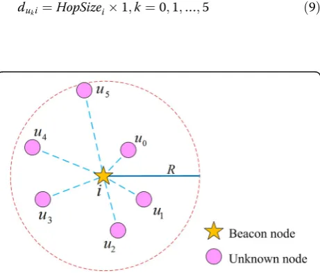
node, there are many unknown nodes in its communica-tion radius, and the distance between these unknown nodes and the beacon node is not completely equal. However, when the distance between them is calculated according to the principle of DV-Hop algorithm, the ob-tained results are equal. The reason is that, within the communication radius of the beacon node, the hop values between all unknown nodes and the beacon node will be recorded as 1 hop, and these unknown nodes are closest to the beacon node. Therefore, when calculating the distance from the beacon node, they use the average hop distance broadcasted by the beacon node. Because the product of hop value and average hop distance be-tween two nodes is regarded as the distance bebe-tween two nodes, which makes the distance between these un-known nodes and beacon nodes be equal. Taking Fig.2 as an example, all the hop values between unknown nodesu0,u1, ..., u5and beacon node iare 1 hop.
More-over, when calculating the distance between these un-known nodes and beacon nodes, the average hop distanceHopSizeof beacon node iis employed, so there are:
duki¼HopSizei1;k¼0;1;…;5 ð9Þ
Then, we can get:
du0i¼du1i;Λ;¼du5i ð10Þ
This is not matched with the actual distance value be-tween unknown nodes u0, u1, ..., u5and beacon node i.
In fact, the distance between them should satisfy the fol-lowing relationship:
du0i<du1iΛ<du5i ð11Þ
As can be seen from Fig. 2, the distance between u0,
u1, ..., u5and node iis quite different, so it is necessary
to adjust the hop value between them according to the distance between nodes, instead of simply recording all the hops as 1.
2. The error of average hop distance
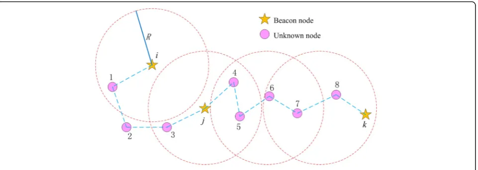
When calculating the distance between the unknown node and the beacon node, the average hop distance from the near-est beacon node is adopted, so the rationality of the average hop distance determines the location error of the unknown node. Taking Fig.3 as an example, the influence of average hop distance on distance calculation between unknown nodes and beacon nodes is illustrated. Wherei,j, and krepresent beacon nodes, numbers 1, 2,..., 8 represent unknown nodes, and the communication radius between any two nodes is set asR. As can be seen from Fig.3, the ideal hop value between beacon nodeiand beacon nodejis only slightly greater than one hop, but the hop value between beacon nodeiand bea-con nodejis 4 due to the random distribution of nodes. For beacon nodejand beacon nodek, their ideal hop value are about 3, but the actual network topology shows that the hop value between them is 6. According to the principle of DV-Hop algorithm, the average hop distance of jcan be calcu-lated as (‖ij‖+‖jk‖)/(4 + 6). However, in ideal case, the average hop distance ofjis about (‖ij‖+‖jk‖)/(1 + 3). There-fore, the actual average hop distance calculated is less than the average hop distance in ideal case. For the unknown nodes 3 and 4 which are nearest to the beacon node, they use the average hop distance to calculate the distance between them and beacon nodej, which is expressed by (‖ij‖+‖jk‖)/
Fig. 1Network topology diagram
(4 + 6) × 1≈4R/10. Meanwhile, the actual distance between unknown nodes 3 and 4 and beacon nodejis almostR, so the calculated distance is far less than the actual distance. Similarly, the average hop distances of beacon nodesiandk are different from the actual average hop distances, so employing the average hop distance of unknown nodes will also cause errors when calculating the distance between un-known nodes and beacon nodes.
3. The calculation error of node position
Because the distance data between unknown nodes and beacon nodes is obtained by means of estimation, there is a certain deviation between the estimated distance and the actual distance. If the method used in calculating the coor-dinates of unknown nodes is inappropriate, the error may further increase.
Maximum likelihood estimation error analysis diagram is showed as Fig.4.
The positioning error by means of maximum likelihood method is illustrated by Fig.4. SupposeA1(x1,y1),A2(x2,y2),...,
Am(xm,ym) are the beacon nodes, the unknown node isU(x,
y), and the estimated distance between the unknown node and the beacon nodes isd1, d2, …, dm, whose errors
com-pared with the actual distances are ε1,ε2.….εm, respectively.
Therefore, the following equations can be obtained from the relationship between the actual distance and the estimated distance:
x−x1
ð Þ2þ
y−y1
ð Þ2¼
d21þγ21 x−x2
ð Þ2þ
y−y2
ð Þ2¼
d22þγ22 M
x−xm
ð Þ2þ
y−ym
ð Þ2¼
d2mþγ2m 8
> > < > >
: ð
12Þ
By subtracting the first (m-1) term from the last one respectively, the following linear equations can be obtained:
2ðx1−xmÞxþ2ðy1−ymÞy¼x21−x 2
mþy
2 1−y
2
mþd
2
m−d
2 1þγ
2
m−γ
2 1 2ðx2−xmÞxþ2ðy2−ymÞy¼x22−x
2
mþy
2 2−y
2
mþd
2
m−d
2 2þγ
2
m−γ
2 2 M
2ðxm−1−xmÞxþ2ðym−1−ymÞy¼x2m−1−xm2þy2m−1−y2mþd2m−d2m−1þγ2m−γ2m−1
8 > > < > > :
ð13Þ
From the above equation, we can see that each equa-tion contains an error term:
δk ¼γ2m−γ2k;k∈½1;m−1 ð14Þ
Whereγ2
k¼ 2dkεkþε2k,k∈[1,m−1]. Therefore, due to the existence of the above error term, the error in the new equation is larger than that of any of the original two subtractive equations. Therefore, the error between the coordinates of unknown nodes obtained by this method and the actual values increases.
3 DV-Hop location algorithm based on minimum hop thinning and average distance correction
Based on the above analysis on error problem, this paper improves the DV-Hop algorithm by using minimum hop thinning and average hop distance correction.
3.1 Minimum hop thinning
The shadowing model is shown as Eq. (15).
Fig. 3Network topology diagram for an example
Prð Þd0
Where d is the distance between any two nodes that need to measure distance, d0 is a reference distance
be-tween two nodes,Pr(d) represents a power corresponding
to distanced,Pr(d0) represents a power corresponding to
distanced0,k0is a path loss factor, and its value is
gener-ally set between 2 and 6.
In Eq. (15), a random noise with a mean of 0 and a standard deviation ofσis introduced, and Xis generally used to represent the random distribution. If the dis-tance from the transmitting end is d, the receiving power of the receiving end will bePr(d)dB, wheredB
rep-resents power and d0 = 1m. Meanwhile, if the average
RSSI value of Areceiving end is 1m from the transmit-ting end, the RSSI value at dfrom the transmitting end will be deduced from Eq. (15):
Prð Þ ¼d A−10k0 lgdþXσ ð16Þ
Generally, the RSSI value decreases along with the in-creasing distance from the transmitter. Therefore, un-known nodes can calculate the distance from beacon nodes by using RSSI value. Next, according to the above method, the hop value of DV-Hop location algorithm will be corrected.
1. Grading the first hop
In this paper, the general idea of improving the hop value is to weigh the hop value h1of the first hop. The
ideal distance of the first hop is the communication ra-diusR, which is the same as all nodes in the whole net-work. Therefore, by grading the communication radius R, each stage corresponds to a hop value, which can re-duce the impact of hops on positioning error and im-prove positioning accuracy.
Let the communication radius of the node be R, and the distance (not the hop distance) between the node and its neighbor node be x. When the hop number of the first hop is counted ash1and the first hop is divided
into mlevels, the hop number of the first hop is shown in Eq. (17).
Whereiis a positive integer less thanm.
In the actual application process, there is no way to obtain distance. Equation (16) reflects the relationship between
distance and power, so there isði−m1ÞR<x≤iR
m, where the cor-responding RSSI value is concerned as seen in Eq. (18).
A−10k0lg
In practical applications, the power caused by Gauss noise is very small, which is smaller than the power value corresponding to the first hop, so the influence of Gauss noise on the hop value can be completely ignored. From Eqs. (17) and (18), the relationship between the hop num-ber of the first hop and the receiving power of the corre-sponding sensor node can be obtained as seen in Eq. (19).
hi¼
Equation (19) classifies the first hop of sensor node ac-cording to the attenuation intensity of RSSI signal. This method makes the hop value of traditional DV-Hop al-gorithm become decimal, which improves the position-ing accuracy of the nodes to be positioned and reduces the error. At the same time, the hop valueh1of the first
hop can be used to correct the rest of the hops.
2. Weighting the hop value
Define the weight: If the hop value between sensor nodes in the network is greater than 1 hop, then the weightHjis defined as the ratio of the distancedjofjhop
measured by RSSI technology to the first hop distanced1,
which can be seen in Eq. (20).
Hj¼ dj
d1 ð20Þ
Wherejis a positive integer.
According to Eq. (15), Eq. (20) is further transformed to obtain the relationship between distance and receiving power. The RSSI received by the receiving node at dis-tancedfrom the sending node is represented byPr(d)dB,
as shown in Eq. (21).
d d0¼10
Pr dð Þ0−Pr dð ÞdB
10k0 ð21Þ
Hj¼ dj d1¼
10Prð Þd0 −Prð Þd dB
10k0 ð
22Þ
Equation (22) is the weight calculation formula of hop value between nodes. Moreover, the weight must be the weight of the hop value between the node and its neigh-bors. By multiplying the weight with the hop valueh1of
the first hop, the hop value of this hop can be obtained, and the distance between sensor nodes in the whole net-work can be corrected.
3.2 Average distance correction
If the number of beacon nodes in the monitoring area is n, the average hop distance of each beacon node in the whole network will be calculated by Eq. (1). Let the aver-age hop distance of all beacon nodes be recorded asDavg
as shown in Eq. (23).
Davg ¼ 1 n
Xn
i¼1
HopSizei ð23Þ
Let the difference between the average hop distance of beacon nodei and the Davg value calculated by Eq. (23)
be recorded asDi1, which is shown in Eq. (24).
Di1¼ HopSizei−Davg
2
ð24Þ
Let the difference between the actual distance and the estimated distance between beacon nodes iandj in the whole network be recorded as Di2, which is shown in
Eq. (25).
Di2¼ 1 n−1
X
i≠j
dij−^dij hopij
!
ð25Þ
Among them,dijis the actual distance between beacon
nodei andj. d^ij¼HopSizeihopij is the estimated dis-tance between beacon node i and j; hopij is the
mini-mum hop between beacon nodeiandj.
If the weight of beacon node i is ωi, the error
coeffi-cient of this beacon node will be obtained by Eqs. (25) and (26), and the weightωican be obtained by using this
error coefficient, as shown in Eq. (26).
ωi¼
1
1þ1=ðDi1þDi2Þ ð
26Þ
The average hop distance between beacon nodesiand jis redefined as Eq. (27).
Avghopsizeij¼
ffiffiffiffiffiffiffiffiffiffiffiffiffiffiffiffiffiffiffiffiffiffiffiffiffiffiffiffiffiffiffiffiffiffiffiffiffiffiffiffi xi−xj
2
þ yi−yj
2
r
1þ1=ðDi1þDi2Þ ð
27Þ
Let the average hop distance of the re-estimated bea-con node i be Avginew, which is a weighted value of the
error coefficient of each beacon node in the whole net-work. Moreover, it is calculated by combing with Eq. (27), and is shown in Eq. (28).
Avginew¼ Xn−1
j
ωjAvghopsizeij
Xn−1
j ωj
ð28Þ
If the coordinates of unknown node and beacon node are (xk,yk) and (xi,yi) respectively, the hop distance from
un-known nodekto beacon nodeiwill be shown in Eq. (29).
dki¼hopkiAvginew ð29Þ
Wherekandiare variables.
4 Experiment results and analysis
In Matlab environment, 200 sensor nodes are randomly distributed in a square area of 200 m × 200 m. The pro-portion of initial beacon nodes to total nodes increases from 0.05 to 0.3, the communication radius R = 30 m. The relationship between the average positioning error of the whole network and the proportion of initial bea-con nodes is shown in Fig. 5. Figure 5 shows that the average positioning error of the two algorithms de-creases with the increase of the proportion of beacon nodes. Furthermore, under the same proportion of bea-con nodes, the average positioning error of the DV-Hop algorithm in this paper is smaller than that of the trad-itional DV-Hop algorithm.
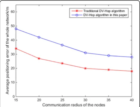
Under the same environment, 200 sensor nodes are randomly distributed in the square area of 200 m × 200 m. The proportion of beacon nodes to total nodes is 0.1. The communication radiusRincreases from 15 to 40 m.
The relationship between the average positioning error of the whole network and the communication radius of the nodes is shown in Fig. 6. Figure 6 shows that the average positioning error of the two algorithms de-creases with the increase of the communication radius of the nodes. When the communication radius reaches a certain value, the decline trend of the average position-ing error of the whole network is gradually smooth. Moreover, when the communication radius is the same, the average positioning error of the DV-Hop algorithm in this paper is less than that of the traditional DV-Hop algorithm.
5 Conclusion
Aiming at the disadvantage of large error existing in the traditional wireless sensor network location algorithm based on Hop, this paper proposes an improved DV-Hop algorithm based on hop thinning and distance cor-rection. The minimum hop is corrected by introducing RSSI ranging technology, and the average hop distance is corrected by weighted average value of hop distance error and estimated distance error. The experimental results show that the improved algorithm reduces the location error and has higher location accuracy.
Abbreviations
DV-Hop:Distance vector hop; RSSI: Received signal strength indication; WSN: Wireless sensor network
Acknowledgements Not applicable.
Authors’contributions
The author completed the experiment and manuscript. The author read and approved the final manuscript.
Authors’information
Dalong Xue: PhD student, School of Computer Science and Technology, Beijing Institute of Technology. His research interests include computer network technology, software algorithm.
Funding Not applicable.
Availability of data and materials
The data generated and analyzed during this study are included in this published article, and its supplementary information is also available from the corresponding author on reasonable request.
Competing interests
The author declares that he has no competing interest.
Received: 13 June 2019 Accepted: 16 August 2019
References
1. A. Kaur, P. Kumar, G.P. Gupta, Nature inspired algorithm-based improved
variants of DV-Hop algorithm for randomly deployed 2D and 3D wireless
sensor networks[J]. Wireless Personal Communications101(1), 567–582 (2018)
2. G. Sharma, A. Kumar, Improved DV-Hop localization algorithm using
teaching learning based optimization for wireless sensor networks[J].
Telecommunication Systems67(2), 163–178 (2018)
3. J. Mass-Sanchez, E. Ruiz-Ibarra, J. Cortez-Gonzalez, A. Espinoza-Ruiz, L.A. Castro,
Weighted hyperbolic DV-Hop positioning node localization algorithm in
WSNs[J]. Wireless Personal Communications96(4), 5011–5033 (2017)
4. R. Kaur, J. Malhotra, Comparitive analysis of DV-hop and APIT localization
techniques in WSN [J]. International Journal of Future Generation
Communication and Networking.9(8), 327–344 (2016)
5. A. Kaur, G.P. Gupta, P. Kumar, A Survey of Recent Developments In DV-Hop
localization techniques for wireless sensor network[J]. Future Generation
Computer Systems9(2), 61–71 (2017)
6. J. Mass-Sanchez, E. Ruiz-Ibarra, J. Cortez-González, et al., Weighted
hyperbolic DV-Hop positioning node localization algorithm in WSNs[J].
Wireless Personal Communications96(2), 5011–5033 (2016)
7. S. Kumar, D.K. Lobiyal, Power efficient range-free localization algorithm for
wireless sensor networks[J]. Wireless Networks20(4), 681–694 (2014)
8. S. Tomic, I. Mezei, Improvements of DV-Hop localization algorithm for
wireless sensor networks[J]. Telecommunication Systems61(1), 93–106
(2016)
9. H. Adachi, H. Suzuki, K. Asahi, et al., Estimation of bustraveling section using
wireless sensor network[J]. Eighth International Conference on IEEE, 120–
125 (2015)
10. S. Gayan, D. Dias, Improved DV-Hop algorithm through anchor position
re-estimation[C]. 2014 IEEE Asia Pacific Conference on IEEE, 126–131 (2014)
11. F. Darakeh, G.R. Mohammad-Khani, P. Azmi, CRWSNP: cooperative range-free
wireless sensor network positioning algorithm[J]. Wireless Networks13(1),
1–17 (2017)
12. S. Kumar, D.K. Lobiyal, Novel DV-Hop localization algorithm for wireless
sensor networks[J]. Telecommunication Systems16(23), 1–16 (2016)
Publisher’s Note
Springer Nature remains neutral with regard to jurisdictional claims in published maps and institutional affiliations.