Simpler Software Analytics: When? When Not?

ABSTRACT

FU, WEI. Simpler Software Analytics: When? When not?. (Under the direction of Dr. Timothy Menzies.)

Software engineering researchers and industrial practitioners routinely make extensively use of software analytics to discover insights about their projects: how long it will take to develop their code, or where bugs are most likely to occur. Significant research effort has been put forth to improve the quality of model software analytics. There has been continuous development of new feature selection, feature discovering and even new modeling techniques for software analytics. These exciting innovations have the potential to dramatically improve the quality of software analytics tools. The problem is that most of these methods are complex (e.g.,): not easy to explain, hard to reproduce, and require large amount of computational resources.

In this dissertation,we want to investigate the potential of simpler software analytics. The thesis of this dissertation is that software analytics should be simpler; Software analytics can be simpler; However, oversimplification can be harmful. To defend the claim of the thesis, we have conducted several studies to explore simple tools in different tasks, like software defect prediction and software text mining.

First of all, we discuss why software analytics should be simpler. From the perspectives of effectiveness, economy, explainability and reproducibility, we argue that simpler software analytics have more potential to impact the software engineering industry. To show software analytics can be simpler, we conduct a study to simplify hyper-parameter tuning techniques on software defect prediction tasks. According to our literature review, hyper-parameter tuning was ignored in most software defect prediction works. Even though some researchers proposed methods to tune learners’ hyper-parameters, those methods usually take at least hours to complete, which would not motivate researchers to tune hyper-parameters in every single task. In this dissertation, we proposed to apply search-based software engineering method, like differential evolution algorithm, to tune defect predictors. According to the experiment, we usually get better performance than predictors with default parameters. Meanwhile, tuning with differential evolution can be terminated within seconds or minutes on defect prediction tasks, which requires far less resources than most frequently used hyper-parameter tuning techniques proposed by other researchers.

between different questions posted on Stack Overflow. First of all, it is hard to select a case study like the one we studied to explore simplicity versus complexity because most papers using complex methods (e.g., deep learning) do not share either the source code or data, which could introduce bias if we explore the same topic with different datasets or implement the proposed method. In this tudy, even though we got the same testing data from the author we compared wtih, we are still missing training data. Therefore, to fully reproduce the experiment, we spend months of time in collecting data, pre-processing data and reproducing the prior study. Based on the experimental resutls, we find that tuning simple learner with differential evolution algorithm outperforms the deep learning method for this task while our proposed method is 84 times faster. This conclusion further confirms that our first claim that software analytics can be simpler and complex software analytics methods can be improved and outperformed by simpler methods. Since most existing software analytics research tends to be more complex and not fully open-sourced, showing any single software analytics tasks can be simplified is not simple at all.

Thirdly, we show that simplification for software analytics can be done in a harmful way. Specifi-cally, over-simplification without considering the local information can generate a less effective model. By reproducing a recent study in FSE’16 about just-in-time effort aware defect prediction, we find that the unsupervised predictors proposed in the original paper can not get a consistent prediction among all proposed unsupervised learners. To improve their method, we investigated the use of local data to prune weak predictors and only select the best one as the final predictor. Experimental results show that our proposed simple method,OneWay, performs better than the unsupervised learners as well as more complex standard supervised learners. Through this study, we defend our claim that software analytics can be simpler but can not be oversimplified.

© Copyright 2018 by Wei Fu

Simpler Software Analytics: When? When not?

by Wei Fu

A dissertation submitted to the Graduate Faculty of North Carolina State University

in partial fulfillment of the requirements for the Degree of

Doctor of Philosophy

Computer Science

Raleigh, North Carolina

2018

APPROVED BY:

Dr. Min Chi Dr. Christopher Parnin

Dr. Ranga Vatsavai Dr. Timothy Menzies

DEDICATION

BIOGRAPHY

ACKNOWLEDGEMENTS

A Five-year PhD study is a special journey in my life. I could not finish it without the support and encouragement from many nice people I meet over this time. Therefore, I would like to thank the following people.

I am grateful to my advisor, Dr. Tim Menzies, for the time and effort he took in introducing me to software engineering research, for all his enthusiasm, patience, advice, and funding. That means a lot to me. Our story informally started from the moment that I followed him on Facebook in 2014 summer. Back then, I was down and about to quit my PhD program while he just started his career at NC State. As his first NC State graduate student who happened to have no computer science background, he always patiently explains every single knowledge/idea that I could not understand. Sometimes, even repeating English words until I get them. Over past four years,he raised me up, so that I can stand on mountains; He raised me up to more than I can be. This thesis could not have been possible without his help on every single step during my PhD study.

I am grateful to my PhD committee members, Dr. Min Chi, Dr. Chris Parnin, and Dr. Raju Vatsavai, for all the time spent, all the help and advice on my research and career.

I am grateful to the members of Dr. Tim Menzies’ RAISE lab: Vivek Nair, Rahul Krishna, George Mathew, Jianfeng Chen, Zhe Yu, Amritanshu Agrawal, Di Chen, Tianpei Xia, Huy Tu, Suvodeep Majumder, and our distinguished visiting scholar, Dr. Junjie Wang. Thanks for all the critiques on my work, project collaboration, and even paper proof reading. Those tears, beers, woes, and joys that we shared together are great moments that will never be forgot. I am grateful to the RAISE Lab founding members: Vivek Nair, Rahul Krishna and George Mathew, who taught me not only the new computer skills but also the old Indian culture. I will miss those days and nights that I stood around and listened to random research discussions in room 3231, even though most of them turned out to not work at all. Special thanks to Vivek Nair, who has been serving as my “vice-advisor” over past 4 years when the actual one is not on. I wish I could put him on my committee even though our first co-authored work went nowhere.

I am grateful to my friends I made at NC State. This list can only be partial: Qiang(Jack) Zhang, Junjiamin Mu, Chen(Liana) Lin, Feifei Wang, Shengpei Zhang, Qiong Tao, Kelei Gong, Jiaming Li, Pei Deng, Xing Pan, Peipei Wang, Hui Guan, Liang Dong, Xiaozhou Fang, Hong Xiong, Xin Xu, Akhilesh Tanneeru, Adam Gillfillan. Thanks for your invaluable support, advice, and inspiring ideas. Those are really important during my whole PhD study, especially my tough time.

we still keep in touch and the tremendous support from this group of friends keeps me moving forward. Special thanks to Dr. Feifei Gao from Tsinghua University, I could not even start my PhD study without his advice, encouragement and recommendation.

TABLE OF CONTENTS

LIST OF TABLES . . . ix

LIST OF FIGURES. . . xi

Chapter 1 Introduction. . . 1

1.1 Background . . . 1

1.1.1 Software Analytics . . . 1

1.1.2 Defect Prediction . . . 2

1.2 Contributions . . . 5

I Software Analytics Should Be Simpler 8 Chapter 2 The Quest for Simplicity in Software Analytics . . . 9

II Software Analytics Can Be Simpler 12 Chapter 3 Tuning for Software Analytics . . . 13

3.1 Introduction . . . 14

3.2 Preliminaries . . . 15

3.2.1 Tuning: Important and Ignored . . . 15

3.2.2 You Can’t Always Get What You Want . . . 16

3.2.3 Notes on Data Miners . . . 18

3.2.4 Learners and Their Tunings . . . 18

3.2.5 Tuning Algorithms . . . 21

3.3 Experimental Design . . . 23

3.3.1 Data Sets . . . 23

3.3.2 Optimization Goals . . . 24

3.4 Experimental Results . . . 24

3.4.1 RQ1: Does Tuning Improve Performance? . . . 24

3.4.2 RQ2: Does Tuning Change a Learner’s Ranking ? . . . 25

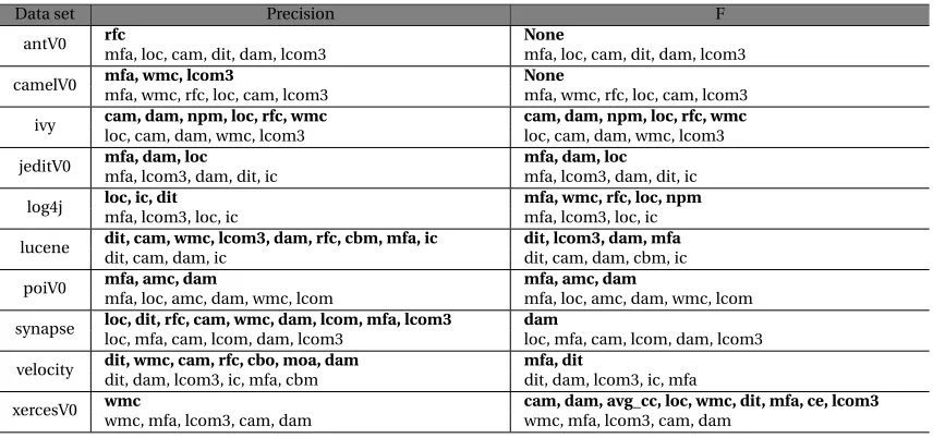
3.4.3 RQ3: Does Tuning Select Different Project Factors? . . . 28

3.4.4 RQ4: Is Tuning Easy? . . . 29

3.4.5 RQ5: Is Tuning Impractically Slow? . . . 30

3.4.6 RQ6: Should we use “off-the-shelf” Tunings? . . . 32

3.5 Reliability and Validity . . . 33

3.6 Conclusions . . . 33

Chapter 4 Differential Evolution V.S. Grid Search . . . 35

4.1 Introduction . . . 36

4.2 Background . . . 38

4.2.2 Parameter Tuning . . . 39

4.3 Method . . . 41

4.3.1 Algorithms . . . 41

4.3.2 Data Miners . . . 42

4.3.3 Tuning Parameters . . . 43

4.3.4 Data . . . 43

4.3.5 Optimization Goals . . . 44

4.3.6 20 Random Runs: . . . 45

4.3.7 Statistical Tests . . . 45

4.4 Results . . . 46

4.5 Discussion . . . 50

4.5.1 Why does DE perform better than grid search? . . . 50

4.5.2 When (not) to use DE? . . . 51

4.6 Threats to Validity . . . 54

4.7 Conclusion . . . 55

Chapter 5 Easy Over Hard. . . 56

5.1 Introduction . . . 57

5.2 Background and Related Work . . . 58

5.2.1 Why Explore Faster Software Analytics? . . . 58

5.2.2 What is Deep Learning? . . . 59

5.2.3 Deep Learning in SE . . . 60

5.2.4 Parameter Tuning in SE . . . 63

5.3 Method . . . 64

5.3.1 Research Problem . . . 64

5.3.2 Learners and Their Parameters . . . 65

5.3.3 Learning Word Embedding . . . 65

5.3.4 Tuning Algorithm . . . 67

5.4 Experimental Setup . . . 68

5.4.1 Research Questions . . . 68

5.4.2 Dataset and Experimental Design . . . 68

5.4.3 Evaluation Metrics . . . 70

5.5 Results . . . 71

5.6 Discussion . . . 77

5.6.1 Why DE+SVM works? . . . 77

5.6.2 Implication . . . 78

5.6.3 Threads to Validity . . . 78

5.7 Conclusion . . . 79

III However, Oversimplification Can Be Harmful 80 Chapter 6 Unsupervised Learners. . . 81

6.1 Introduction . . . 82

6.3 Background and Related Work . . . 84

6.3.1 Defect Prediction . . . 84

6.3.2 Just-In-Time Defect Prediction . . . 85

6.4 Method . . . 86

6.4.1 Unsupervised Predictors . . . 86

6.4.2 Supervised Predictors . . . 88

6.4.3 OneWay Learner . . . 88

6.5 Experimental Settings . . . 89

6.5.1 Research Questions . . . 89

6.5.2 Data Sets . . . 90

6.5.3 Experimental Design . . . 91

6.5.4 Evaluation Measures . . . 92

6.6 Empirical Results . . . 93

6.7 Threats to Validity . . . 102

6.8 Conclusion and Future Work . . . 102

IV Future Work and Conclusion 104 Chapter 7 Future Work . . . .105

7.1 Introduction . . . 106

7.2 Background . . . 108

7.2.1 Different Defect Prediction Approaches . . . 108

7.2.2 Evaluation Criteria . . . 109

7.2.3 Sources ofεUncertainty . . . 111

7.3 ε-Domination . . . 113

7.4 Experimental Setup . . . 115

7.4.1 Research Questions . . . 116

7.4.2 Datasets . . . 117

7.5 Results . . . 117

7.5.1 RQ1: Do established learners sample results space better than a few DARTs? . 117 7.5.2 RQ2: Do goal-savvy learners sample results space better than a few DARTs? . . 119

7.5.3 RQ3: Do data-savvy learners sample results space better than a few DARTs? . 121 7.6 Threads to Validity . . . 123

7.7 Discussion and Future Work . . . 124

Chapter 8 Conclusion. . . .127

LIST OF TABLES

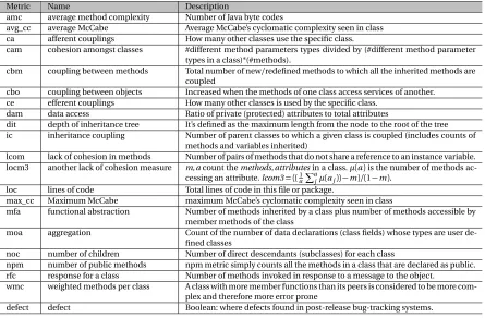
Table 1.1 OO Measures used in our defect data sets. . . 4

Table 3.1 List of parameters tuned by this study. . . 19

Table 3.2 Data used in this experiment. E.g., the top left data set has 20 defective classes out of 125 total. See §3.3.1 for explanation oftraining, tuning, testingsets. . . 23

Table 3.3 Precision results (best results shown inbold). . . 26

Table 3.4 F-measure results (best results shown inbold). . . 26

Table 3.5 Features selected by tuned WHERE with different goals:boldfeatures are those found useful by the tuned WHERE. Also, features shown in plain text are those found useful by the untuned WHERE. . . 28

Table 3.6 Kolmogorov-Smirnov Tests for distributions of Figure 3.3 . . . 30

Table 3.7 Number of evaluations for tuned learners, optimizing for precision and F-Measure. 31 Table 3.8 Runtime for tuned and default learners(in sec), optimizing for precision and F-Measure. . . 31

Table 4.1 List of parameters tuned by this study. . . 39

Table 4.2 Data used in this case study. . . 43

Table 5.1 Classes of knowledge unit pairs. . . 64

Table 5.2 List of parameters tuned by this study. . . 64

Table 5.3 Confusion matrix. . . 70

Table 5.4 Comparison of our baseline method with XU’s. The best scores are marked inbold. 72 Table 5.5 Comparison of the tuned SVM with XU’s CNN method. The best scores are marked inbold. . . 74

Table 5.6 Comparison of experimental environment . . . 76

Table 6.1 Change metrics used in our data sets. . . 87

Table 6.2 Statistics of the studied data sets . . . 90

Table 6.3 Comparison inPo p t: Yang’s method (A) vs. our implementation (B) . . . 94

Table 6.4 Comparison inRecall: Yang’s method (A) vs. our implementation (B) . . . 94

Table 6.5 Best unsupervised predictor (A) vs. OneWay (B). The colorful cell indicates the size effect: green for large; yellow for medium; gray for small. . . 97

Table 6.6 Best supervised predictor (A) vs. OneWay (B). The colorful cell indicates the size effect: green for large; yellow for medium; gray for small. . . 100

Table 7.1 32 defect predictors clustered by their performance rank by Ghotra et al. (using a Scott-Knot statistical test)[Gho15]. . . 108

Table 7.2 Statistics of the studied data sets. . . 118

Table 7.3 DART v.s. state-of-the-art defect predictors from Ghotra et al.[Gho15]fordis2heaven andPopt. Gray cells mark best performances on each project (so DART is most-often best). . . 118

Table 7.5 DART v.s. tuning Random Forests fordis2heavenandPopt. Gray cells mark best performances on each project. Note that even when DART does not perform best, it usually performs very close to the best. . . 122 Table 7.6 DART v.s. data-savvy learners indist2heavenandPopt. Gray cells mark best

LIST OF FIGURES

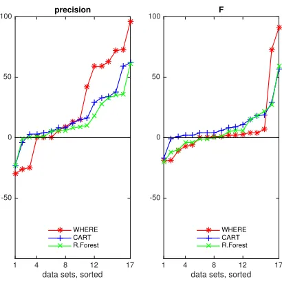
Figure 3.1 Deltas in performance seen in Table 3.3 (left) and Table 3.4 (right) between tuned and untuned learners. Tuning improves performance when the deltas are above

zero. . . 25

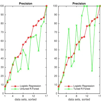
Figure 3.2 Comparison between Logistic Regression and Random Forest before and after tuning. . . 27

Figure 3.3 Deltas in performance betweennp=10and the recommended np’s. The rec-ommended np is better when deltas are above zero.np =90, 50 and 60are recommended population size for WHERE, CART and Random Forest by Storn. . 29

Figure 3.4 Four representative tuning values in WHERE with precision and F-measure as the tuning goal, respectively. . . 32

Figure 4.1 Literature review about parameter tuning on 52 top cited defect prediction papers 40 Figure 4.2 Tuning to improveF. Median results from 20 repeats. . . 45

Figure 4.3 Tuning to improvePrecision. Median results from 20 repeats. . . 46

Figure 4.4 Tuning to improveAUC. Median results from 20 repeats. . . 47

Figure 4.5 Tuning to improveAUC₂₀. Median results from 20 repeats. . . 47

Figure 4.6 Time (in seconds) required to run 20 repeats of parameter tunings for learners to generate Figure 4.2 to Figure 4.5. . . 48

Figure 4.7 Runtime relative to just running the learners using their default tunings. . . 49

Figure 4.8 Intrinsic dimensionality of our data. . . 52

Figure 4.9 Illustration for data D=dimensionality . . . 52

Figure 5.1 Procedure TUNER: strives to find “good” tunings which maximizes the objec-tive score of the model on training and tuning data. TUNER is based on Storn’s differential evolution optimizer[SP97]. . . 67

Figure 5.2 The overall workflow of building knowledge units predictor with tuned SVM. . . . 69

Figure 5.3 Score delta between our SVM with XU’s SVM in [Xu16]in terms of precision, recall and F1-score. Positive values mean our SVM is better than XU’s SVM in terms of different measures; Otherwise, XU’s SVM is better. . . 72

Figure 5.4 Score delta between tuned SVM and CNN method[Xu16]in terms of precision, recall and F1-score. Positive values mean tuned SVM is better than CNN in terms of different measures; Otherwise, CNN is better. . . 74

Figure 5.5 Score delta between the tuned SVM and XU’s baseline SVM in terms of precision, recall and F1-score. Positive values mean the tuned SVM is better than XU’s SVM in terms of different measures; Otherwise, XU’s SVM is better. . . 75

Figure 5.6 Score delta between tuned SVM and Our Untuned SVM in terms of precision, re-call and F1-score. Positive values mean the tuned SVM is better than our untuned SVM in terms of different measures; Otherwise, our SVM is better. . . 75

Figure 6.1 Example of an effort-based cumulative lift chart [Yan16b]. . . 92

Figure 6.3 Performance comparisons between the proposedOneWaylearner and unsu-pervised predictors over six projects (from top to bottom are Bugzilla, Platform,

Mozilla, JDT, Columba, PostgreSQL). . . 98

Figure 6.4 Performance comparisons between the proposedOneWaylearner and super-vised predictors over six projects (from top to bottom are Bugzilla, Platform, Mozilla, JDT, Columba, PostgreSQL). . . 100

Figure 7.1 Illustration ofPo p t metric. . . 109

Figure 7.2 Illustration ofdis2heavenmetric. . . 110

Figure 7.3 Results space when recall is greater than false alarms (see blue curve). . . 111

Figure 7.4 Grids in results space. . . 113

Figure 7.5 εcan vary across results space. 100 experiments with LUCENE results using 90% of the data, for training, and 10%, for testing. The x-axis sorts the code base, first according to predicted defective or not, then second on lines of code. The blue line shows the distribution of the 100 results across this space. For example, 70% of the results predict defect for up to 20% of the code (see the blue curve). The y-axis of this figures shows mean recall (in red); the standard deviations i g m a of the recall (in yellow); andεis defined as per standard t-tests that says at the 95% confidence level, two distributions differ when they areε=2∗1.96∗σapart. (in green). . . 114

Figure 7.6 DART: an ensemble algorithm to sample results space,M number of times. . . 116

Figure 7.7 A simple model for software defect prediction . . . 116

Figure 7.8 TUNER is an evolutionary optimization algorithm based on Storn’s differential evolution algorithm[SP97; FM17b]. . . 121

CHAPTER

1

INTRODUCTION

1.1

Background

1.1.1 Software Analytics

In the 21s t century, it is impossible to manually browse all available software project data. The SeaCraft repository of SE data has grown to 200+projects[Sea]and this is just one of over a dozen open-source repositories that are readily available to researchers[Rod12]. Faced with this data over-load, researchers in empirical software engineering field and software practitioners used analytics, like data mining tools, to generate models to get better understanding of the software projects. According to Menzies et al.[MZ13a], software analytics is defined as:“software analytics is analytics on software data for managers and software engineers with the aim of empowering software devel-opment individuals and teams to gain and share insight from their data to make better decisions.” Software analytics have been applied to many applications in Software Engineering (SE). For example, it has been used to estimate how long it would take to integrate new code into an existing project[Cze11a], where defects are most likely to occur[Ost04; Men07c], which two questions asked by software developers are related[Xu16], or how long will it take to develop a project[Tur11; Koc12a], etc. Large organizations, like Microsoft, routinely practice data-driven policy development where organizational policies are learned from an extensive analysis of large data sets[BZ14; The15a].

it harder for the users to reproduce models, understand models or operatinalize models. For example, there are some evidence to show that deep learning methods are very effective for building software analytics models based on high dimensional data[Xu16; Wan16; Gu16]. However, since most deep learning methods have very complex structures and a tiny difference may lead to a huge difference in the results. For example, different weights initialization schemes will have great impacts on the speed of network convergence. Therefore, it is hard to reproduce the invented models by a third-party if the original research paper did not share the model; furthermore, most deep learning methods require weeks of hours of GPU/CPU time to train a model on a moderate size of data set[Xu16], much of that GPU/CPU time can be saved if there is a faster method for this analytics. Therefore, the total financial cost of training deep learning models can be prohibitive, particularly for long running tasks. In addition, the most obvious drawback of deep learning methods is that they do not readily support explainability, they have been criticizing as “data mining alchemy”[Syn17]. At a recent workshop on “Actionable Analytics” at ASE’15, business users were very vocal in their complaints about analytics[HM15], saying that there are rarely producible models that business users can understand or operationalize.

In software analytics, if a model is to be used to persuade software engineers to change what they are doing, it needs to becomprehensibleso humans can debate the merits of its conclusions. Several researchers demand that software analytics models needs to be expressed in a simple way that is easy for software practitioners to interpret[Men14a; Lip16; Dam18]. According to Kim et al.[Kim16], software analytics aim to obtain actionable insights from software artifacts that help practitioners accomplish tasks related to software development, systems, and users. Other researchers[TC16] argue that for software vendors, managers, developers and users, such comprehensible insights are the core deliverable of software analytics. Sawyer et al. comments that actionable insight is the key driver for businesses to invest in data analytics initiatives[Saw13]. Accordingly, much research focuses on the generation of simple models, or making blackbox models more explainable, so that human engineers can understand and appropriately trust the decisions made by software analytics models[FM17b; AN16].

Based the drawbacks we discussed above, we think that we need simple, actionable, and ex-plainable software analytics models. Therefore, for software researchers and practitioners, it is the time to simplify software analytics from the perspectives ofeffectiveness,economy,explainability andreproducibility. In this dissertation, I will show what I have learned about simplicity in software analytics.

1.1.2 Defect Prediction

Human programmers are clever, but flawed. Coding adds functionality, but also defects. Hence, software sometimes crashes (perhaps at the most awkward or dangerous moment) or delivers the wrong functionality. For a very long list of software-related errors, see Peter Neumann’s “Risk Digest” at catless.ncl.ac.uk/Risks.

Since programming inherently introduces defects into programs, it is important to test them before they are used. Testing is expensive. Software assessment budgets are finite while assessment effectiveness increases exponentially with assessment effort. For example, for black-box testing methods, alinearincrease in the confidenceC of finding defects can takeexponentiallymore effort:

• A randomly selected input to a program will find a fault with probabilityp.

• AfterN random black-box tests, the chances of the inputs not revealing any fault is(1−p)N. • Hence, the chancesC of seeing the fault is 1−(1−p)N which can be rearranged toN(C,p) =

l o g(1−C)/l o g(1−p).

• For example,N(0.90, 10−3) =2301 butN(0.98, 10−3) =3901; i.e. nearly double the number of tests.

Exponential costs quickly exhaust finite resources so standard practice is to apply the best available methods on code sections that seem most critical. But any method that focuses on parts of the code can blind us to defects in other areas. Somelightweight sampling policyshould be used to explore the rest of the system. This sampling policy will always be incomplete. Nevertheless, it is the only option when resources prevent a complete assessment of everything.

One such lightweight sampling policy is defect predictors learned from static code attributes. Given software described in the attributes of Table 1.1, data miners can learn where the probability of software defects is highest. The rest of this section argues that such defect predictors areeasy to use,widely-used, andusefulto use.

Easy to use: Static code attributes can be automatically collected, even for very large sys-tems[NB05a]. Other methods, like manual code reviews, are far slower and far more labor-intensive. For example, depending on the review methods, 8 to 20 LOC/minute can be inspected and this effort repeats for all members of the review team, which can be as large as four or six people[Men02].

Widely used:Researchers and industrial practitioners use static attributes to guide software quality predictions. Defect prediction models have been reported at Google[Lew13]. Verification and validation (V&V) textbooks[Rak01]advise using static code complexity attributes to decide which modules are worth manual inspections.

Table 1.1OO Measures used in our defect data sets.

Metric Name Description

amc average method complexity Number of Java byte codes

avg_cc average McCabe Average McCabe’s cyclomatic complexity seen in class ca afferent couplings How many other classes use the specific class.

cam cohesion amongst classes #different method parameters types divided by (#different method parameter types in a class)*(#methods).

cbm coupling between methods Total number of new/redefined methods to which all the inherited methods are coupled

cbo coupling between objects Increased when the methods of one class access services of another. ce efferent couplings How many other classes is used by the specific class.

dam data access Ratio of private (protected) attributes to total attributes

dit depth of inheritance tree It’s defined as the maximum length from the node to the root of the tree ic inheritance coupling Number of parent classes to which a given class is coupled (includes counts of

methods and variables inherited)

lcom lack of cohesion in methods Number of pairs of methods that do not share a reference to an instance variable. locm3 another lack of cohesion measure m,acount themethods,attributesin a class.µ(a)is the number of methods

ac-cessing an attribute.lcom3= ((a1 Pa

jµ(aj))−m)/(1−m).

loc lines of code Total lines of code in this file or package.

max_cc Maximum McCabe maximum McCabe’s cyclomatic complexity seen in class

mfa functional abstraction Number of methods inherited by a class plus number of methods accessible by member methods of the class

moa aggregation Count of the number of data declarations (class fields) whose types are user de-fined classes

noc number of children Number of direct descendants (subclasses) for each class

npm number of public methods npm metric simply counts all the methods in a class that are declared as public. rfc response for a class Number of methods invoked in response to a message to the object.

wmc weighted methods per class A class with more member functions than its peers is considered to be more com-plex and therefore more error prone

in finding bugs is markedly higher than other currently-used industrial methods such as manual code reviews. For example, a panel atIEEE Metrics 2002[Shu02]concluded that manual software reviews can find≈60% of defects. In another work, Raffo documents the typical defect detection capability of industrial review methods: around 50% for full Fagan inspections[Fag76]to 21% for less-structured inspections.

Not only do static code defect predictors perform well compared to manual methods, they also are competitive with certain automatic methods. A recent study at ICSE’14, Rahman et al.[Rah14] compared (a) static code analysis tools FindBugs, Jlint, and Pmd and (b) static code defect predictors (which they called “statistical defect prediction”) built using logistic regression. They found no significant differences in the cost-effectiveness of these approaches. Given this equivalence, it is significant to note that static code defect prediction can be quickly adapted to new languages by building lightweight parsers that find information like Table 1.1. The same is not true for static code analyzers– these need extensive modification before they can be used on new languages.

1.2

Contributions

Over my past five-year PhD study, I was trying to demonstrate how to reach such goal by using simple techniques to make software analytics easy. Based on those studies, I formulated the following thesis:

Software analytics should be simpler;

Software analytics can be simpler; However, oversimplification can be harmful.

In the above, by “simpler” we mean simple methods over complex methods. simple methods mean fast, requiring less computational resources, reproducible, and easy to explain and understand; and complex emthoes mean slow, requiring days to weeks of CPU time to execute, not reproducible, not easy to explain and undertand;

This dissertation advances knowledge by several contributions. To defend thatSoftware analytics can be simpler, I offer evidence through two case studies:

• Tuning for Software Analytics: The performance of software analytics can be improved from various perspectives and by different ways. On direction to reach this goal is to tune hyper-parameters of existing software analytics methods. In Chapter 3, we show that by applying one simple search-based software engineering method, differential evolution (DE), to tune software quality prediction methods, the detection precision of the resulting models are improved from 0% to 60% on different datasets.

analytics, it is still a quite under-explored problem. After the success with differential evolution for tuning software analytics, we did a literature review on parameter tuning methods for software quality prediction. We found that 94% papers we surveyed did not conduct parameter tuning and 4% papers mentioned that grid search was applied to to tune parameters. Since it’s easy to understand and implement and, to some extent, also has good performance, grid search has been available in most popular data mining and machine learning tools, likecaret[Kuh14] package in theRandGridSearchCVmodule in Scikit-learn[Ped11]. In Chapter 3, we want to evaluate which method can find better parameters in terms ofeffectiveness(performance score) andeconomy(runtime cost). Experimental results show that the seemingly complete approach of grid search does no better, and sometimes worse, than differential evolution method. Since the best results from grid search are largely depending ongrid pointsset by the user. Grid search is prone to skip optimal configurations and waste time exploring useless space. On the other hand, with the DE method, users do not need to use expert knowledge to set thegrid pointsand the method itself will explore the searching space automatically. We are not going to sell DE as the best parameter tuning, but at least, it’s a good candidate for considering trade off between performance and runtime. Through this case study, we show that, simple hyper-parameter tuning methods, like differential evolution, perform no worse than resource consuming grid search method for hyper-parameter tuning.

To defend the claim thatsimpler methods can reach parity with complex methods with much lower execution costs and less understanding barriers, I offer the evidence through the following case study on text mining tasks:

Easy Over Hard: In Chapter 4, we extend a prior result from ASE’16 by Xu et al.[Xu16]. In their work, they described a deep learning method to explore large programmer discussion forums, then uncover related, but separate, entries. In this study, we spend weeks of time to collect, clean, and transform data from Stack Overflow. We strictly followed Xu et al.’s description to split data and train the Word2vec model. To show that simple techniques work better than complex ones, we apply DE to tune SVM model(which was used to serve as baseline method in Xu’s paper). We show here that applying a very simple optimizer DE to fine tune SVM, it can achieve similar (and sometimes better) results. The DE approach terminated in 10 minutes (while that deep learning system took 14 hours to execute.); i.e. 84 times faster hours than deep learning method.

To defend the claim thatHowever, oversimplification can be harmful, I offer the evidence through the following case study on software quality prediction tasks:

that learn models from project data labeled with, say, “defective” or “not-defective” for software quality prediction tasks. Most researchers use these supervised models since, it is argued, they can exploit more knowledge of the projects. At FSE’16, Yang et al. reported startling results where unsupervised defect predictors outperformed supervised predictors for effort-aware just-in-time defect prediction. If confirmed, these results would lead to a dramatic simplification of a seemingly complex task (data mining) that is widely explored in the software engineering literature. In Chapter 5, we repeat and refute Yang et al. results: (1) There is much variability in the efficacy of the Yang et al. unsupervised predictors so even with their approach, some supervised data is required to prune weaker predictors away. (2) Their findings were grouped acrossN projects. When we repeat their analysis on a project-by-project basis, supervised predictors are seen to work better. Therefore, when taking actions to simplify software analytics, we need to use caution to avoid pitfalls and make models more applicable.

Simplifying software analytics is not an easy task itself. Sometimes, we find that some methods work, most of time, it does not. Therefore, it is necessary to have a criterion or indicator to tell us when simple methods could work. We were trying to explore this question, and in the following study, we show some preliminary results in this direction:

Part I

CHAPTER

2

THE QUEST FOR SIMPLICITY IN

SOFTWARE ANALYTICS

In this chpater, we argue thatsoftware analytics should be simpler. We study simplicity since it is very useful to replaceN methods withM N methods, especially when the results from the many are no better than the few. Take a software quality prediction task as an example. Each year, a bewildering array of new methods for software quality prediction are reported (some of which rely on intimidatingly complex mathematical methods) such as deep belief net learning[Wan16], spectral-based clustering[Zha16], and n-gram language models[Ray16]. Ghotra et al. list dozens of different data mining algorithms that might be used for defect predictors[Gho15]. Fu and Menzies argue that these algorithms might require extensive tuning[Fu16a]. There are many ways to implement that tuning, some of which are very slow[Tan16]. And if they were not enough, other computationally expensive methods might also be required to handle issues like (say) class imbalance[AM18].

to cost”[Fis12]. Fisher et al. [Fis12]document the issues seen by 16 industrial data scientists, one of whom remarks

“Fast iteration is key, but incompatible with the jobs are submitted and processed in the cloud. It is frustrating to wait for hours, only to realize you need a slight tweak to your feature set”.

Methods for improving the quality of modern software analytics have made this issue even more serious. There has been continuous development of new feature selection[HH03]and feature discovering[Jia13]techniques for software analytics, with the most recent ones focused on deep learning methods. These are all exciting innovations with the potential to dramatically improve the quality of our software analytics tools. Yet these are all CPU/GPU-intensive methods. For instance:

• Learning control settings for learners can take days to weeks to years of CPU time[Fu16b; Tan16; Wan13b].

• Lam et al. needed weeks of CPU time to combine deep learning and text mining to localize buggy files from bug reports[Lam15].

• Gu et al. spent 240 hours of GPU time to train a deep learning based method to generate API usage sequences for given natural language query[Gu16].

Power consumption and heat dissipation issues effect block further exponential increases to CPU clock frequencies[Kum03]. Cloud computing environments are extensively monetized so the total financial cost of training models can be prohibitive, particularly for long running tasks. For example, it would take 15 years of CPU time to learn the tuning parameters of software clone detectors proposed in [Wan13b]. Much of that CPU time can be saved if there is a faster way.

Given recent advances in cloud computing, it is possible to find the best method for a particular data set via a “shoot out” between different methods. For example, Lessmann et al.[Les08]and Ghotra et al.[Gho15]explored 22 and 32 different learning algorithms (respectively) for software quality defect prediction. Such studies may require days to weeks of CPU time to complete[FM17b]. But are such complex and time-consuming studies necessary?

• If there exists some way to dramatically simplify software quality predictors; then those cloud-based resources would be better used for other tasks.

• Also, Lessmann and Ghotra et al.[Les08; Gho15]report that many defect prediction methods have equivalent performance.

Another reason to study simplification is that studies can reveal the underlying nature of seem-ingly complex problems. In terms of core science, we argue that the better we understand something, the better we can match tools to SE. Tools which are poorly matched to task are usually complex and/or slow to execute.

Seeking simpler and/or faster solutions is not just theoretically interesting. It is also an approach currently in vogue in contemporary software engineering. Calero and Pattini[CP15]comments that “redesign for greater simplicity” also motivates much contemporary industrial work. In their survey of modern SE companies, they find that many current organizational redesigns are motivated (at least in part) by arguments based on “sustainability” (i.e., using fewer resources to achieve results). According to Calero and Pattini, sustainability is now a new source of innovation. Managers used sustainability-based redesigns to explore cost-cutting opportunities. In fact, they say, sustainability is now viewed by many companies as a mechanism for gaining a complete advantage over their competitors. Hence, a manager might ask a programmer to assess simple methods to generate more interesting products.

Part II

CHAPTER

3

TUNING FOR SOFTWARE ANALYTICS

This chapter firstly appeared atInformation and Software Technology 76 (2016): 135-146titled “Tuning for software analytics: is it really necessary?”. In this chapter, by using this study, we want to

show that software analytics can be easier.

3.1

Introduction

One of the “black arts” of data mining is setting the tuning parameters that control the choices within a data miner. Prior to this work, our intuition was that tuning would change the behavior or a data miner, to some degree. Nevertheless, we rarely tuned our defect predictors since we reasoned that a data miner’s default tunings have been well-explored by the developers of those algorithms (in which case tuning would not lead to large performance improvements). Also, we suspected that tuning would take so long time and be so CPU intensive that the benefits gained would not be worth effort.

The results of this study show that the above points are false since, at least for defect prediction from code attributes:(1) Tuning defect predictors isremarkably simple; (2) And candramatically improve the performance. Those results were found by exploring six research questions:

• RQ1:Does tuning improve the performance scores of a predictor? We will show below examples of truly dramatic improvement: usually by 5 to 20% and often by much more (in one extreme case, precision improved from 0% to 60%).

• RQ2:Does tuning change conclusions on what learners are better than others?Recent SE pa-pers[Les08; Hal12]claim that some learners are better than others. Some of those conclusions are completely changed by tuning.

• RQ3:Does tuning change conclusions about what factors are most important in software engineering?Numerous recent SE papers (e.g.[Bel13; RD13; MS03; Mos08; Zim07; Her13]) use data miners to conclude thatthisis more important thanthatfor reducing software project defects. Given the tuning results of this study, we show that such conclusions need to be revisited.

• RQ4:Is tuning easy?We show that one of the simpler multi-objective optimizers (differential evolution[SP97]) works very well for tuning defect predictors.

• RQ5:Is tuning impractically slow?We achieved dramatic improvements in the performance scores of our data miners in less than 100 evaluations (!); i.e., very quickly.

• RQ6:Should data miners be used “off-the-shelf” with their default tunings?For defect predic-tion from static code measures, our answer is an emphatic “no” (and the implicapredic-tion for other kinds of analytics is now an open and urgent question).

for conducting such tunings; (3) Tuning needs to be repeated whenever data or goals are changed. Fortunately, the cost of finding good tunings is not excessive since, at least for static code defect predictors, tuning is easy and fast.

3.2

Preliminaries

3.2.1 Tuning: Important and Ignored

This section argues that tuning is an under-explored software analytics– particularly in the apparently well-explored field of defect prediction.

In other fields, the impact of tuning is well understood[BB12]. Yet issues of tuning are rarely or poorly addressed in the defect prediction literature. When we tune a data miner, what we are really doing is changing how a learner applies its heuristics. This means tuned data miners use different heuristics, which means they ignore different possible models, which means they return different models; i.e.howwe learn changeswhatwe learn.

Are the impacts of tuning addressed in the defect prediction literature? To answer that question, in Jan 2016 we searched scholar.google.com for the conjunction of “data mining" and “software engineering" and “defect prediction" (more details can be found at https://goo.gl/Inl9nF). After sorting by the citation count and discarding the non-SE papers (and those without a pdf link), we read over this sample of 50 highly-cited SE defect prediction papers. What we found in that sample was that few authors acknowledged the impact of tunings (exceptions:[Gao11; Les08]). Overall, 80% of papers in our sampledid notadjust the “off-the-shelf” configuration of the data miner (e.g.[Men07b; Mos08; EE08]). Of the remaining papers:

• Some papers in our sample explored data super-sampling[PD07]or data sub-sampling tech-niques via automatic methods (e.g. [Gao11; Men07b; PD07; Kim11]) or via some domain principles (e.g. [Mos08; Nag08; Has09]). As an example of the latter, Nagappan et al.[Nag08] checked if metrics related to organizational structure were relatively more powerful for pre-dicting software defects. However, it should be noted that these studies varied the input data but not the “off-the-shelf” settings of the data miner.

navigate the large space of possible tunings.

Over our entire sample, there was only one paper that conducted a somewhat extensive tuning study. Lessmann et al.[Les08]tuned parameters for some of their algorithms using agrid search; i.e. divide allC configuration options intoN values, then try allNC _{combinations. This is a slow approach–} we have explored grid search for defect prediction and found it takes days to terminate[Men07b]. Not only that, we found that grid search can miss important optimizations[Bak07]. Every grid has “gaps” between each grid division which means that a supposedly rigorous grid search can still miss important configurations[BB12]. Bergstra and Bengio[BB12]comment that for most data sets only a few of the tuning parameters really matter– which means that much of the runtime associated with grid search is actually wasted. Worse still, Bergstra and Bengio comment that the important tunings are different for different data sets– a phenomenon that makes grid search a poor choice for configuring data mining algorithms for new data sets.

Since the Lessmann et al. paper, much progress has been made in configuration algorithms and we can now report thatfinding useful tunings is very easy. This result is both novel and unexpected. A standard run of grid search (and other evolutionary algorithms) is that optimization requires thousands, if not millions, of evaluations. However, in a result that we found startling, thatdifferential evolution(described below) can find useful settings for learners generating defect predictors in less than 100 evaluations (i.e. very quickly). Hence, the “problem” (that tuning changes the conclusions) is really an exciting opportunity. At least for defect prediction, learners are very amenable to tuning. Hence, they are also very amenable to significant performance improvements. Given the low number of evaluations required, then we assert that tuning should be standard practice for anyone building defect predictors.

3.2.2 You Can’t Always Get What You Want

Having made the case that tuning needs to be explored more, but before we get into the technical details of this paper, this section discusses some general matters about setting goals during tuning experiments.

This study characterizes tuning as an optimization problem (how to change the settings on the learner in order to best improve the output). With such optimizations, it is not always possible to optimize for all goals at the same time. For example, the following text does not show results for tuning on recall or false alarms since optimizingonlyfor those goals can lead to some undesirable side effects:

• False alarmsis the percentage of other examples that are reported (by the learner) to be part of the targeted examples. When we tune forfalse alarms, we can achieve near zero percent false alarm rates by effectively turning off the detector (so the recall falls to nearly zero).

Accordingly, this study explores performance measures that comment on all target classes: see the precision and “F” measures discussed below: seeOptimization Goals. That said, we are sometimes asked what good is a learner if it optimizes for (say) precision at the expense of (say) recall.

Our reply is that software engineering is a very diverse enterprise and that different kinds of development need to optimize for different goals (which may not necessarily be “optimize for recall”):

• Anda, Sjoberg and Mockus are concerned withreproducibilityand so assess their models using the the “coefficient of variation” (CV=stddev_mean) [And09].

• Arisholm & Briand[AB06], Ostrand & Weyeuker[Ost04]and Rahman et al.[Rah12]are con-cerned with reducing the work load associated with someone else reading a learned model, then applying it. Hence, they assess their models usingreward; i.e. the fewest lines of code containing the most bugs.

• Yin et al. are concerned aboutincorrect bug fixes; i.e. those that require subsequent work in order to complete the bug fix. These bugs occur when (say) developers try to fix parts of the code where they have very little experience[Yin11]. Hence, they assess a learned model using a measure that selects for the most number of bugs in regions thatthe most programmers have worked with before.

• For safety critical applications, high false alarm rates are acceptable if the cost of overlooking critical issues outweighs the inconvenience of inspecting a few more modules.

• When rushing a product to market, there is a business case to avoid the extra rework associated with false alarms. In that business context, managers might be willing to lower the recall somewhat in order to minimize the false alarms.

• When Dr. Menzies worked with contractors at NASA’s software independent verification and validation facility, he found new contractors only reported issues that were most certainly important defects; i.e. they minimized false alarms even if that damaged their precision (since, they felt, it was better to be silent than wrong). Later on, once those contractors had acquired a reputation of being insightful members of the team, they improved their precision scores (even if it means some more false alarms).

Rather, what we can show examples where changing optimization goals can also change the conclusions made from that learner on that data. More generally, we caution that it is important not to overstate empirical results from analytics. Those results need to be expressedalong withthe context within which they are relevant (and by “context”, we mean the optimization goal).

3.2.3 Notes on Data Miners

There are several ways to make defect predictors using CART[Bre01], Random Forest[Bre84], WHERE[Men13]and LR (logistic regression). For this study, we use CART, Random Forest and LR versions from SciKitLearn[Ped11]and WHERE, which is available from github.com/ai-se/where. We use these algorithms for the following reasons.

CART and Random Forest were mentioned in a recent IEEE TSE paper by Lessmann et al.[Les08] that compared 22 learners for defect prediction. That study ranked CART worst and Random Forest as best. In a demonstration of the impact of tuning, this study shows we canrefutethe conclusions of Lessmann et al. in the sense that, after tuning, CART performs just as well as Random Forest.

LR was mentioned by Hall et al.[Hal12]as usually being as good or better as more complex learners (e.g. Random Forest). In a finding that endorses the Hall et al. result, we show that untuned LR performs better than untuned Random Forest (at least, for the data sets studied here). However, we will show that tuning raises doubts about the optimality of the Hall et al. recommendation.

Finally, this paper uses WHERE since, as shown below, it offers an interesting case study on the benefits of tuning.

3.2.4 Learners and Their Tunings

Our learners use the tuning parameters of Table 3.1 The default parameters for CART and Random Forest are set by the Scikit-learn authors and the default parameters for WHERE-based learner are set via our own expert judgment. When we say a learner is used “off-the-shelf”, we mean that they use the defaults shown in Table 3.1.

As to the value of those defaults, it could be argued that these defaults are not the best parameters for practical defect prediction. That said, prior to this study, two things were true:

• Many data scientists in SE use the standard defaults in their data miners, without tuning (e.g.[Men07b; Mos08; Her13; Zim07]).

• The effort involved to adjust those tunings seemed so onerous, that many researchers in this field were content to take our prior advice of “do not tune... it is just too hard”[Men14b].

Table 3.1List of parameters tuned by this study.

Learner Name Parameters Default Tuning

Range Description

Where-based Learner

threshold 0.5 [0.01,1] The value to determine defective or not .

infoPrune 0.33 [0.01,1] The percentage of features to consider for the best split to build its final decision tree.

min_sample_split 4 [1,10] The minimum number of samples required to split an inter-nal node of its fiinter-nal decision tree.

min_Size 0.5 [0.01,1] Finds min_samples_leaf in the initial clustering tree using

n_samplesmin_Size.

wriggle 0.2 [0.01, 1] The threshold to determine which branch in the initial clus-tering tree to be pruned

depthMin 2 [1,6] The minimum depth of the initial clustering tree below which no pruning for the clustering tree.

depthMax 10 [1,20] The maximum depth of the initial clustering tree. wherePrune False T/F Whether or not to prune the initial clustering tree.

treePrune True T/F Whether or not to prune the final decision tree.

CART

threshold 0.5 [0,1] The value to determine defective or not.

max_feature None [0.01,1] The number of features to consider when looking for the best split.

min_sample_split 2 [2,20] The minimum number of samples required to split an inter-nal node.

min_samples_leaf 1 [1,20] The minimum number of samples required to be at a leaf node.

max_depth None [1, 50] The maximum depth of the tree.

Random Forests

threshold 0.5 [0.01,1] The value to determine defective or not.

max_feature None [0.01,1] The number of features to consider when looking for the best split.

max_leaf_nodes None [1,50] Grow trees with max_leaf_nodes in best-first fashion. min_sample_split 2 [2,20] The minimum number of samples required to split an

inter-nal node.

min_samples_leaf 1 [1,20] The minimum number of samples required to be at a leaf node.

n_estimators 100 [50,150] The number of trees in the forest. Logistic Regression This study uses untuned LR in order to check a conclusion of[Hal12].

largertuning ranges might not result ingreaterimprovements. However, for the goals of this study (to show that some tunings do matter), exploring just these ranges shown in Table 3.1 will suffice.

As to the details of these learners, LR is a parametric modeling approach. Givenf =β₀+P

iβixi, wherexiis some measurement in a data set, andβiis learned via regression, LR converts that into a function 0≤g≤1 usingg=1/ 1+e−f. This function reports how much we believe in a particular class.

inspect=







d_i≥T →Yes di<T →No,

(3.1)

wheredi is the number of observed issues andT is some threshold defined by an engineering judgment; we useT =1.

The splitting process is controlled by numerous tuning parameters. If data contains more than min_sample_split, then a split is attempted. On the other hand, if a split contains no more than min_-samples_leaf, then the recursion stops. CART and Random Forest use a user-supplied constant for this parameter while WHERE-based learner firstly computes this parameterm=min_samples_leaf from the size of the data sets viam=sizemin_sizeto build an initial clustering tree. Note that WHERE buildstwotrees: the initial clustering tree (to find similar sets of data) then a final decision tree (to learn rules that predict for each similar cluster). A frequently asked question is why does WHERE build two trees– would not a single tree suffice? The answer is, as shown below, tuned WHERE’s twin-tree approach generates very precise predictors. As to the rest of WHERE’s parameters, the parameter min_sample_ split controls the construction of the final decision tree (so, for WHERE-based learner, min_sizeandmin_sample_splitare the parameters to be tuned).

These learners use different techniques to explore the splits: CART finds the attributes whose ranges contain rows with least variance in the number of defects. If an attribute rangesriis found inni rows each with a defect count variance ofvi, then CART seeks the attributes whose ranges minimizesP

i pvi×ni/(

P

ini)

; Random Forest divides data like CART then buildsF >1 trees, each time using some random subset of the attributes; When building the initial cluster tree, WHERE projects the data on to a dimension it synthesizes from the raw data using a process analogous to principle component analysis[Jol02]. WHERE divides at the median point of that projection. On recursion, this generates the initial clustering tree, the leaves of which are clusters of very similar examples. After that, when building the final decision tree, WHERE pretends its clusters are “classes”, then asks the InfoGain algorithm of the Fayyad-Irani discretizer[FI93], to rank the attributes, where infoPruneis used. WHERE’s final decision tree generator then ignores everything except the top infoPrunepercent of the sorted attributes.

and its parent have the same majority cluster (one that occurs most frequently), then iftree_prune is enabled, we prune that decision sub-tree.

3.2.5 Tuning Algorithms

How should researchers select which optimizers to apply to tuning data miners? Cohen[Coh95] advises comparing new methods against the simplest possible alternative. Similarly, Holte[Hol93] recommends using very simple learners as a kind of “scout” for a preliminary analysis of a data set (to check if that data really requires a more complex analysis). Accordingly, to find our “scout”, we used engineering judgement to sort candidate algorithms from simplest to complex. For example, here is a list of optimizers used widely in research:simulated annealing[FM02; Men07a]; various genetic algorithms[Gol79]augmented by techniques such asdifferential evolution[SP97],tabu searchandscatter search[GM86; Bea06a; Mol07; Neb08];particle swarm optimization[Pan08]; numerousdecompositionapproaches that use heuristics to decompose the total space into small problems, then apply aresponse surface methods[Kra15b; Zul13]. Of these, the simplest are simu-lated annealing (SA) and differential evolution (DE), each of which can be coded in less than a page of some high-level scripting language. Our reading of the current literature is that there are more advocates for differential evolution than SA. For example, Vesterstrom and Thomsen[VT04]found DE to be competitive with particle swarm optimization and other GAs.

DEs have been applied before for parameter tuning (e.g. see[Omr05; Chi12]) but this is the first time they have been applied to optimize defect prediction from static code attributes. The pseu-docode for differential evolution is shown in Algorithm 1. In the following description, superscript numbers denote lines in that pseudocode.

DE evolves aNewGenerationof candidates from a currentPopulation. Our DE’s lose one “life” when the new population is no better than current one (terminating when “life” is zero)L4. Each candidate solution in thePopulationis a pair of(Tunings, Scores).Tuningsare selected from Table 3.1 andScorescome from training a learner using those parameters and applying it test dataL23−L27.

The premise of DE is that the best way to mutate the existing tunings is toExtrapolateL28between current solutions. Three solutionsa,b,care selected at random. For each tuning parameteri, at some probabilitycr, we replace the old tuningxi withyi. For booleans, we useyi=¬xi(see line 36). For numerics,y_i =a_i+f ×(b_i−c_i)where f is a parameter controlling cross-over. Thetrim functionL38_{limits the new value to the legal range min..max of that parameter.}

The main loop of DEL6runs over thePopulation, replacing old items with newCandidates (if new candidate is better). This means that, as the loop progresses, thePopulationis full of increasingly more valuable solutions. This, in turn, also improves the candidates, which areExtrapolated from thePopulation.

Algorithm 1Pseudocode for DE with Early Termination

Input:np=10,f=0.75,c r=0.3,life=5,Goal∈ {pd,f, ...}

Output: Sbest

1: functionDE(np,f,cr,life,Goal) 2: Population←InitializePopulation(np)

3: Sb e s t←GetBestSolution(Population)

4: whilelife>0do

5: NewGeneration← ; 6: fori=0→np−1do

7: Si←Extrapolate(Population[i],Population,cr,f)

8: ifScore(Si)>Score(Population[i])then

9: NewGeneration.append(Si)

10: else

11: NewGeneration.append(Population[i]) 12: end if

13: end for

14: Population←NewGeneration 15: if¬Improve(Population)then

16: l i f e−=1 17: end if

18: Sb e s t←GetBestSolution(Population)

19: end while

20: returnSb e s t

21:end function

22:functionSCORE(Candidate)

23: # set tuned parameters according toCandidate 24: model←TrainLearner()

25: result←TestLearner(model) 26: returnGoal(result)

27:end function

28:functionEXTRAPOLATE(old,pop,cr,f) 29: a,b,c←threeOthers(pop,old) 30: newf← ;

31: fori=0→np−1do

32: ifcr<random()then

33: newf.append(o l d[i]) 34: else

35: iftypeof(o l d[i])==boolthen

36: newf.append(notold[i])

37: else

38: newf.append(trim(i,(a[i] +f∗(b[i]−c[i])))) 39: end if

40: end if

41: end for

42: returnnewf 43:end function

Table 3.2Data used in this experiment. E.g., the top left data set has 20 defective classes out of 125 total. See §3.3.1 for explanation oftraining, tuning, testingsets.

Dataset antV0 antV1 antV2 camelV0 camelV1 ivy jeditV0 jeditV1 jeditV2 training 20/125 40/178 32/293 13/339 216/608 63/111 90/272 75/306 79/312 tuning 40/178 32/293 92/351 216/608 145/872 16/241 75/306 79/312 48/367 testing 32/293 92/351 166/745 145/872 188/965 40/352 79/312 48/367 11/492 Dataset log4j lucene poiV0 poiV1 synapse velocity xercesV0 xercesV1

training 34/135 91/195 141/237 37/314 16/157 147/196 77/162 71/440 tuning 37/109 144/247 37/314 248/385 60/222 142/214 71/440 69/453 testing 189/205 203/340 248/385 281/442 86/256 78/229 69/453 437/588

3.3

Experimental Design

3.3.1 Data Sets

Our defect data comes from the PROMISE repository (http://openscience.us/repo/defect) and pertains to open source Java systems defined in terms of Table 1.1:ant,camel,ivy,jedit,log4j,lucene, poi,synapse,velocityandxerces.

An important principle in data mining is not to test on the data used in training. There are many ways to design a experiment that satisfies this principle. Some of those methods have limitations; e.g.leave-one-outis too slow for large data sets andcross-validationmixes up older and newer data (such that data from thepastmay be used to test onfuture data).

To avoid these problems, we used an incremental learning approach. The following experiment ensures that the training data was created at some time before the test data. For this experiment, we use data sets with at least three consecutive releases (where releasei+1 was built after releasei). When tuning a learner, thefirstrelease was used on line 24 of Algorithm 1 to build some model using some the tunings found in someCandidate; Thesecondrelease was used on line 25 of Algorithm 1 to test the candidate model found on line 24; Finally thethirdrelease was used to gather the performance statistics reported below from the best model found by DE.

To be fair for the untuned learner, thefirstandsecondreleases used in tuning experiments will be combined as the training data to build a model. Then the performance of this untuned learner will be evaluated by the samethirdrelease as in the tuning experiment.

Some data sets have more than three releases and, for those data, we could run more than one experiment. For example,anthas five versions in PROMISE so we ran three experiments called V0,V1,V2:

• AntV0: first, second, third=versions 1, 2, 3

• AntV1: first, second, third=versions 2, 3, 4

These data sets are displayed in Table 3.2.

3.3.2 Optimization Goals

Recall from Algorithm 1 that we call differential evolution once for each optimization goal. This section lists those optimization goals. Let{A,B,C,D}denote the true negatives, false negatives, false positives, and true positives (respectively) found by a binary detector. Certain standard measures can be computed fromA,B,C,D, as shown below. Note that forpf, thebetterscores aresmaller while for all other scores, thebetterscores arelarger.

p d=r e c a l l= D/(B+D)

p f= C/(A+C)

p r e c=p r e c i s i o n= D/(D+C)

F= 2∗p d∗p r e c/(p d+p r e c)

The rest of this study explores tuning forprecandF. As discussed in §3.2.2, our point is not that these are best or most important optimization goals. Indeed, the list of “most important” goals is domain-specific (see §3.2.2) and we only explore these two to illustrate how conclusions can change dramatically when moving from one goal to another.

3.4

Experimental Results

In the following, we explore the effects of tuning WHERE, Random Forest, and CART. LR will be used, untuned, in order to check one of the recommendations made by Hall et al.[Hal12].

3.4.1 RQ1: Does Tuning Improve Performance?

Figure 3.1 says that the answer to RQ1 is “yes”– tuning has a positive effect on performance scores. This figure sorts deltas in the precision and the F-measure between tuned and untuned learners. Our reading of this figure is that, overall, tuning rarely makes performance worse and often can make it much better.

Table 3.3 and Table 3.4 show the the specific values seen before and after tuning withprecision and“F”as different optimization goals(the corresponding “F” and precision values for Table 3.3 and Table 3.4 are not provided for the space limitation). For each data set, the maximum precision or “F” values for each data set are shown inbold. As might have been predicted by Lessmann et al.[Les08], untuned CART is indeed the worst learner (only one of its untuned results is best andbold). And, in

12

data sets, sorted

1 4 8 12 17

-50 0 50

100 precision

WHERE CART R.Forest

data sets, sorted

1 4 8 12 17

-50 0 50

100 F

WHERE CART R.Forest

Figure 3.1Deltas in performance seen in Table 3.3 (left) and Table 3.4 (right) between tuned and untuned learners. Tuning improves performance when the deltas are above zero.

That said, tuning can improve those poor performing detectors. In some cases, the median changes may be small (e.g. the “F” results for WHERE and Random Forests) but even in those cases, there are enough large changes to motivate the use of tuning. For example:

• For “F” improvement, there are two improvements over 25% for both WHERE and Random Forests. Also, inpoiV0, all untuned learners report “F” of under 50%, tuning changes those scores by 25%. Finally, note thexercesV1result for the WHERE learner. Here, tuning changes precision from 32% to 70%.

• Regarding precision, forantV0, andantV1untuned WHERE reports precision of 0. But tuned WHERE scores 35 and 60 (the similar pattern can seen in “F”).

3.4.2 RQ2: Does Tuning Change a Learner’s Ranking ?

Researchers often use performance criteria to assert that one learner is better than another[Les08; Men07b; Hal12]. For example:

1. Lessmann et al.[Les08]conclude that Random Forest is considered to be statistically better than CART.

Table 3.3Precision results (best results shown inbold).

WHERE CART Random Forest

Data set default Tuned default Tuned default Tuned

antV0 0 35 15 60 21 44

antV1 0 60 54 56 67 50

antV2 45 55 42 52 56 67

camelV0 20 30 30 50 28 79

camelV1 27 28 38 28 34 27

ivy 25 21 21 26 23 20

jeditV0 34 37 56 78 52 60

jeditV1 30 42 32 64 32 37

jeditV2 4 22 6 17 4 6

log4j 96 91 95 98 95 100

lucene 61 75 67 70 63 77

poiV0 70 70 65 71 67 69

poiV1 74 76 72 90 78 100

synapse 61 50 50 100 60 60

velocity 34 44 39 44 40 42

xercesV0 14 17 17 14 28 14

xercesV1 86 54 72 100 78 27

Table 3.4F-measure results (best results shown inbold).

WHERE CART Random Forest

Data set default Tuned default Tuned default Tuned

antV0 0 20 20 40 28 38

antV1 0 38 37 49 38 49

antV2 47 50 45 49 57 56

camelV0 31 28 39 28 40 30

camelV1 34 34 38 32 42 33

ivy 39 34 28 40 35 33

jeditV0 45 47 56 57 63 59

jeditV1 43 44 44 47 46 48

jeditV2 8 11 10 10 8 9

log4j 47 50 53 37 60 47

lucene 73 73 65 72 70 76

poiV0 50 74 31 64 45 77

poiV1 75 78 68 69 77 78

synapse 49 56 43 60 52 53

velocity 51 53 53 51 56 51

xercesV0 19 22 19 26 34 21

xercesV1 32 70 34 35 42 71

such as Random Forest. To explain that comment, we note that by three measures, Random Forest is more complicated than LR:

(a) CART builds one model while Random Forest builds many models.

(b) LR is just a model construction tool while Random Forest needs both a tool to construct its forestanda second tool to infer some conclusion from all the members of that forest. (c) the LR model can be printed in a few lines while the multiple models learned by Random

Forest model would take up multiple pages of output.