ABSTRACT
AHN, MIHYE. Random Effect Selection in Linear Mixed Models. (Under the direction of Dr. Hao Helen Zhang and Dr. Wenbin Lu.)
The selection of random effects in linear mixed models is an important yet
chal-lenging problem in practice. We propose a robust and unified framework for
au-tomatically selecting random effects and estimating the covariance components in
linear mixed models. A moment-based loss function is constructed for the covariance
parameters of random effects and then a sandwich nonnegative garrote penalty is
imposed for the selection of random effects. Compared to typical approaches, the
new estimator does not require any distribution assumptions on random effects or
the error terms. Large sample theories show that the resulting estimator is consistent
for both random effects selection and variance components estimation. Due to the
nature of variance-covariance matrix of random effects, our procedure involves two
challenging computation problems: nonlinear semidefinite programming and
nonlin-ear programming with a linnonlin-ear inequality constraint. Computational strategies are
suggested to tackle these issues as well as the model tuning. Furthermore, we
pro-pose a natural way to incorporate the selection of fixed effects for the procedure after
choosing random effects. Simulation studies reveal that a better selection of random
effects can yield efficiency gain for the estimation of fixed effects. We use numerous
examples to illustrate the behaviors of the proposed approach and compare it with
existing ones.
and approximating to the original method. Since the objective function in the
origi-nal method has up to fourth order terms and it makes the computation tedious, we
suggest using a linear approximation to the penalized variance-covariance matrix. It
reduces the objective function up to second order, and then the approximate function
can be solved by the quadratic programming in some statistical softwares. We show
that the approximate methods also perform well and often outperform the original
method. Furthermore, the computation speed is remarkably improved in the
approx-imate methods. We finally apply these approaches to a data set from the Amsterdam
Random Effect Selection in Linear Mixed Models
by Mihye Ahn
A dissertation submitted to the Graduate Faculty of North Carolina State University
in partial fulfillment of the requirements for the Degree of
Doctor of Philosophy
Statistics
Raleigh, North Carolina
2010
APPROVED BY:
Dr. Daowen Zhang Dr. Howard Bondell
Dr. Wenbin Lu
Co-Chair of Advisory Committee
DEDICATION
BIOGRAPHY
Mihye Ahn was born in Incheon, South Korea on January 25, 1980. After
gradu-ating from Parkmoon girls’ high school, she began her undergraduate work at Inha
University in statistics. One year later, she decided to double major in business
ad-ministration. When she was a junior, Inha University started to offer the financial
analytics major which is a joint degree program from statistics and business
depart-ments. Mihye also applied to the joint program and finally earned three Bachelor’s
degrees in statistics, business administration, and financial analytics in February 2002.
During her undergraduate studies, she worked as a vice-president of student bodies
in the department of statistics and college of natural science for two years.
Recog-nized leadership and outstanding academic performance, she received the Presidential
Award from Kim Dae-Jung who was ex-president of Korea and the Nobel Peace Prize
laureate.
Mihye continued her graduate work at the same school. She completed her Master
of Science degree in statistics in February 2004 and wrote her thesis ‘Identification of
special causes in dynamic process adjustment with dead time’ under the direction of
Dr. Jae June Lee. Since 2005, she has continued her studies in statistics towards a
ACKNOWLEDGEMENTS
First and foremost I would like to express my deepest gratitude to my advisors, Dr.
Hao Helen Zhang and Dr. Wenbin Lu, for their kind guidance and continuous support
during preparing this dissertation. Whenever I encountered hard problems, they gave
me prompt advice and encouraged me to continue this research. Words cannot express
how lucky I am to have worked with them.
I have to say my sincere thanks to committee members: Dr. Howard Bondell and
Dr. Daowen Zhang for taking their precious time to be on my committee and
pro-viding helpful suggestions. Dr. Tao Pang in mathematics department for attending
my oral preliminary exam and final oral exam as a graduate school representative.
I deeply appreciate Dr. Jae June Lee, my advisor for my master’s thesis at Inha
University. He convinced me to pursue a doctoral degree in the united states. Without
his help, I could not have continued my graduate career. I thank Drs. Hongsuk Jorn,
Jean Kyung Kim, Jinsoo Hwang, Heon Jin Park, and Jinho Park for introducing the
joy of statistics during my time at Inha University.
I would like to thank statistics department at NCSU for providing financial
sup-port during my graduate studies. I could not have completed this work without their
support.
Thanks my friends and colleagues. I regrettably cannot acknowledge individually
by name here, but I would not forget wonderful days with them.
Last but not least, I am very grateful to my parents, my sister and brother for
TABLE OF CONTENTS
List of Tables . . . vii
List of Figures . . . xi
Chapter 1 Introduction . . . 1
1.1 Background . . . 1
1.2 Classical Methods for Fixed Effects Selection . . . 4
1.2.1 Selection Criteria . . . 5
1.2.2 Computational Methods . . . 10
1.3 Penalized Regression for Fixed Effects . . . 12
1.3.1 Ridge Regression . . . 13
1.3.2 Nonnegative Garrote . . . 14
1.3.3 LASSO . . . 15
1.3.4 SCAD . . . 16
1.3.5 Elastic Net . . . 17
1.3.6 Adaptive Lasso . . . 17
1.3.7 OSCAR . . . 18
1.4 Variable Selection in Linear Mixed Models . . . 18
1.4.1 Selection Criteria . . . 19
1.4.2 Penalized Approaches . . . 19
Chapter 2 Random Effects Selection . . . 22
2.1 New Methodology . . . 22
2.2 Asymptotic Properties . . . 26
2.3 Computation & Tuning . . . 30
2.3.1 Algorithm . . . 30
2.3.2 Tuning . . . 31
2.4 Simulation Studies . . . 33
2.4.1 Setting . . . 33
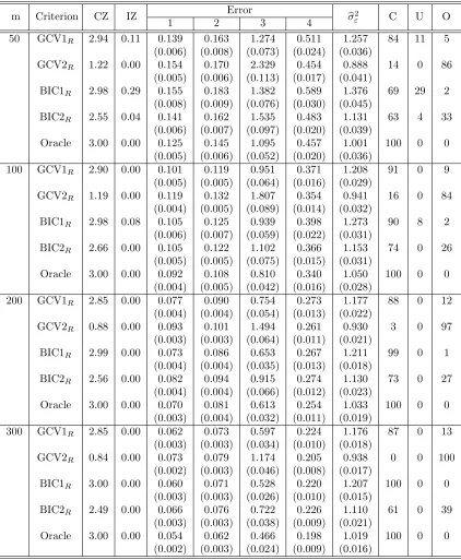
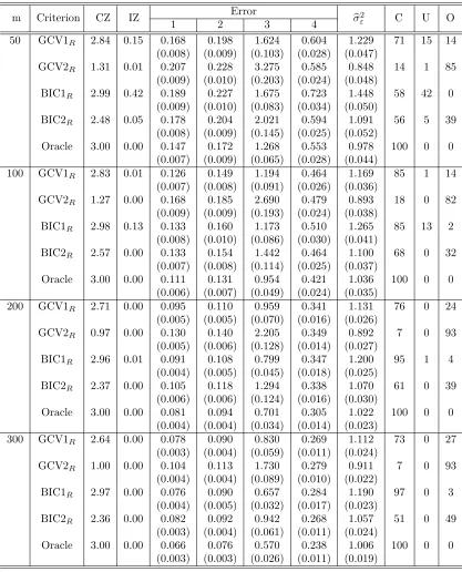
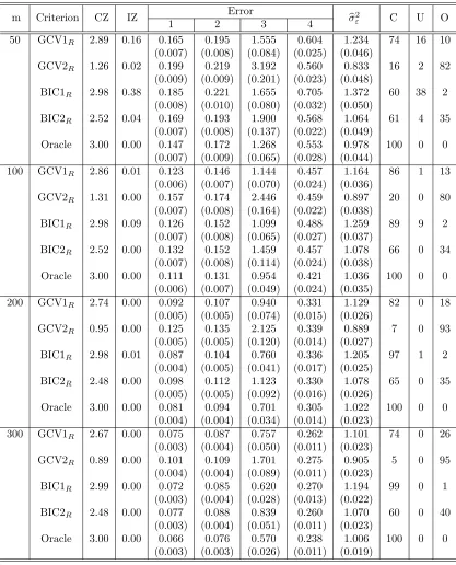
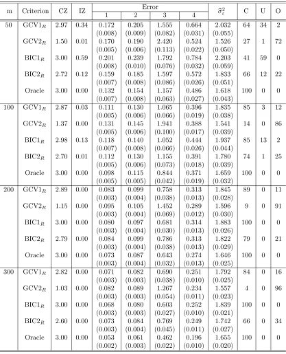
2.4.2 Results . . . 35
Chapter 3 Both Fixed and Random Effects Selection. . . 47
3.1 Methodology and Algorithms . . . 47
3.2 Selection Criteria . . . 49
3.4 Real Example . . . 66
3.4.1 Description . . . 66
3.5 Results . . . 68
Chapter 4 Computationally Efficient Methods for Random Effects Selection in Linear Mixed Models . . . 72
4.1 Motivation . . . 72
4.2 Alternative Efficient Methods . . . 73
4.2.1 Iterative Approximation Method . . . 73
4.2.2 One-step Approximation Method . . . 75
4.3 Simulation Studies . . . 77
4.4 Real Example . . . 94
Chapter 5 Conclusion and Future Work . . . 99
References . . . 101
Appendices . . . 105
Appendix A Asymptotic Properties . . . 106
A.1 Proof of Lemma 1 . . . 106
A.2 Proof of Lemma 2 . . . 108
A.3 Proof of Theorem 1 . . . 112
A.4 Proof of Theorem 2 . . . 116
Appendix B Simulation Results . . . 119
LIST OF TABLES
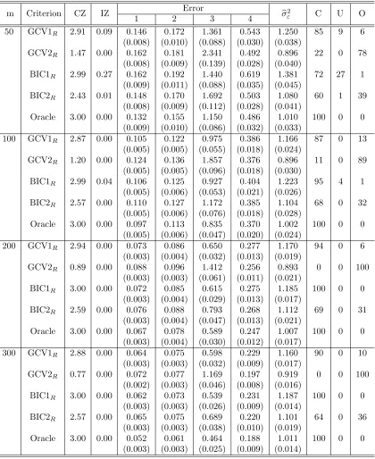
Table 2.1 Random effects selection and estimation results for Setting 1 and Case 1 . . . 37 Table 2.2 Random effects selection and estimation results for Setting 1
and Case 2 . . . 38 Table 2.3 Random effects selection and estimation results for Setting 1
and Case 3 . . . 39 Table 2.4 Random effects selection and estimation results for Setting 1
and Case 4 . . . 40 Table 2.5 Random effects selection and estimation results for Setting 1
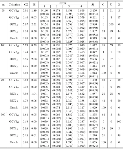
and Case 5 . . . 41 Table 2.6 Random effects selection and estimation results for Setting 2
and Case 1 . . . 42 Table 2.7 Random effects selection and estimation results for Setting 2
and Case 2 . . . 43 Table 2.8 Random effects selection and estimation results for Setting 2
and Case 3 . . . 44 Table 2.9 Random effects selection and estimation results for Setting 2
and Case 4 . . . 45 Table 2.10 Random effects selection and estimation results for Setting 2
and Case 5 . . . 46
Table 3.1 Comparison of Lasso, ALasso1, and ALasso2 for fixed effects selection in Setting 1 . . . 52 Table 3.2 Comparison of Lasso, ALasso1, and ALasso2 for fixed effects
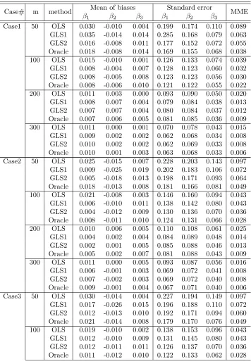
selection in Setting 2 . . . 54 Table 3.3 Biases and standard errors of the estimated fixed-effect
coeffi-cients in Setting 1 . . . 57 Table 3.4 Biases and standard errors of the estimated fixed-effect
coeffi-cients in Setting 2 . . . 59 Table 3.5 Selection and estimation results of both effects for Setting 1 . . 62 Table 3.6 Selection and estimation results of both effects for Setting 2 . . 64 Table 3.7 Comparison of computation times (min/run) for each setting
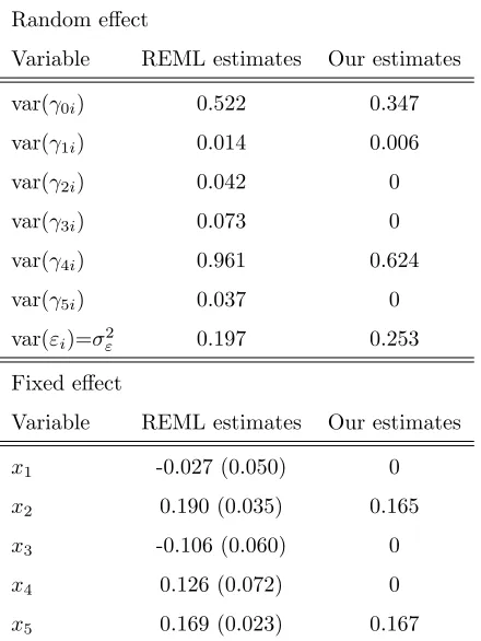
Table 3.8 Mixed effects selection results for the Amsterdam Growth and Health Study data: Comparison of estimates from REML and the proposed methods. Standard errors are given in parentheses 71
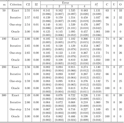
Table 4.1 Random effects selection and estimation results of the exact method and two approximate methods for Setting 1 and Case 1 79 Table 4.2 Random effects selection and estimation results of the exact
method and two approximate methods for Setting 1 and Case 2 80 Table 4.3 Random effects selection and estimation results of the exact
method and two approximate methods for Setting 1 and Case 3 81 Table 4.4 Random effects selection and estimation results of the exact
method and two approximate methods for Setting 1 and Case 4 82 Table 4.5 Random effects selection and estimation results of the exact
method and two approximate methods for Setting 1 and Case 5 83 Table 4.6 Random effects selection and estimation results of the exact
method and two approximate methods for Setting 2 and Case 1 84 Table 4.7 Random effects selection and estimation results of the exact
method and two approximate methods for Setting 2 and Case 2 85 Table 4.8 Random effects selection and estimation results of the exact
method and two approximate methods for Setting 2 and Case 3 86 Table 4.9 Random effects selection and estimation results of the exact
method and two approximate methods for Setting 2 and Case 4 87 Table 4.10 Random effects selection and estimation results of the exact
method and two approximate methods for Setting 2 and Case 5 88 Table 4.11 Fixed effects selection and estimation results of the exact method
and two approximate methods for Setting 1 . . . 90 Table 4.12 Fixed effects selection and estimation results of the exact method
and two approximate methods for Setting 2 . . . 92 Table 4.13 Mixed effects selection results for the Amsterdam Growth and
Health Study data: Comparison of estimates from REML and the proposed methods. Standard errors are given in parentheses 98
Table B.1 Fixed effect selection and estimation results for Setting 1 and Case 1 when applying the Lasso . . . 120 Table B.2 Fixed effect selection and estimation results for Setting 1 and
Case 1 when applying the ALasso1 . . . 121 Table B.3 Fixed effect selection and estimation results for Setting 1 and
Table B.4 Fixed effect selection and estimation results for Setting 1 and Case 2 when applying the Lasso . . . 123 Table B.5 Fixed effect selection and estimation results for Setting 1 and
Case 2 when applying the ALasso1 . . . 124 Table B.6 Fixed effect selection and estimation results for Setting 1 and
Case 2 when applying the ALasso2 . . . 125 Table B.7 Fixed effect selection and estimation results for Setting 1 and
Case 3 when applying the Lasso . . . 126 Table B.8 Fixed effect selection and estimation results for Setting 1 and
Case 3 when applying the ALasso1 . . . 127 Table B.9 Fixed effect selection and estimation results for Setting 1 and
Case 3 when applying the ALasso2 . . . 128 Table B.10 Fixed effect selection and estimation results for Setting 1 and
Case 4 when applying the Lasso . . . 129 Table B.11 Fixed effect selection and estimation results for Setting 1 and
Case 4 when applying the ALasso1 . . . 130 Table B.12 Fixed effect selection and estimation results for Setting 1 and
Case 4 when applying the ALasso2 . . . 131 Table B.13 Fixed effect selection and estimation results for Setting 1 and
Case 5 when applying the Lasso . . . 132 Table B.14 Fixed effect selection and estimation results for Setting 1 and
Case 5 when applying the ALasso1 . . . 133 Table B.15 Fixed effect selection and estimation results for Setting 1 and
Case 5 when applying the ALasso2 . . . 134 Table B.16 Fixed effect selection and estimation results for Setting 2 and
Case 1 when applying the Lasso . . . 135 Table B.17 Fixed effect selection and estimation results for Setting 2 and
Case 1 when applying the ALasso1 . . . 136 Table B.18 Fixed effect selection and estimation results for Setting 2 and
Case 1 when applying the ALasso2 . . . 137 Table B.19 Fixed effect selection and estimation results for Setting 2 and
Case 2 when applying the Lasso . . . 138 Table B.20 Fixed effect selection and estimation results for Setting 2 and
Case 2 when applying the ALasso1 . . . 139 Table B.21 Fixed effect selection and estimation results for Setting 2 and
Case 2 when applying the ALasso2 . . . 140 Table B.22 Fixed effect selection and estimation results for Setting 2 and
Table B.23 Fixed effect selection and estimation results for Setting 2 and Case 3 when applying the ALasso1 . . . 142 Table B.24 Fixed effect selection and estimation results for Setting 2 and
Case 3 when applying the ALasso2 . . . 143 Table B.25 Fixed effect selection and estimation results for Setting 2 and
Case 4 when applying the Lasso . . . 144 Table B.26 Fixed effect selection and estimation results for Setting 2 and
Case 4 when applying the ALasso1 . . . 145 Table B.27 Fixed effect selection and estimation results for Setting 2 and
Case 4 when applying the ALasso2 . . . 146 Table B.28 Fixed effect selection and estimation results for Setting 2 and
Case 5 when applying the Lasso . . . 147 Table B.29 Fixed effect selection and estimation results for Setting 2 and
Case 5 when applying the ALasso1 . . . 148 Table B.30 Fixed effect selection and estimation results for Setting 2 and
LIST OF FIGURES
Figure 3.1 Boxplot of a response variable over subjects . . . 67 Figure 3.2 ∑Profiles of variance matrix estimates for random effects ass =
q
1diis varied. A vertical line is drawn ats= 2.38, the optimal
value chosen by BIC2R . . . 69
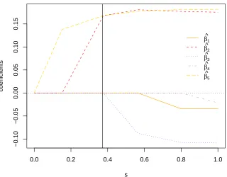
Figure 3.3 Profiles of coefficients for fixed effects for the Amsterdam growth and health study data. A vertical line is drawn ats= 0.37, the optimal value chosen by BIC2F . . . 70
Figure 4.1 ∑Profiles of variance matrix estimates for random effects ass =
q
1di is varied, using the iterative approximation method. A
vertical line is drawn ats = 2.94, the optimal value chosen by BIC2R . . . 95
Figure 4.2 ∑Profiles of variance matrix estimates for random effects ass =
q
1di is varied, using the one-step approximation method. A
vertical line is drawn ats = 2.58, the optimal value chosen by BIC2R . . . 96
Chapter 1
Introduction
1.1
Background
Over the years, variable selection methods have received much attention and been
ap-plied to various fields. Using uninformative variables not only wastes money or time
but also reduce estimation efficiency or prediction accuracy. Selecting an appropriate
set of important variables helps to reduce the variances of parameter estimates. By
deleting some noise variables, we might improve the precision of the estimates.
More-over, a simpler model can enhance model interpretation, and are therefore helpful for
understanding the underlying regression relationship.
When we havepvariables, the total number of possible models is 2p. With a large
number of variables, identifying the optimal model within the large model space can
be computationally burdensome. Sequential procedures, such as forward selection
and backward elimination, can be used for variable selection with relatively less
either added or deleted at a time, and hence provide unstable results. (Breiman,
1995)
For continuous selection process, penalized likelihood methods have been
devel-oped recently, including nonnegative garrote (Breiman, 1995), LASSO Tibshirani
(1996), Fan & Li (2001), Zou & Hastie (2005), Adaptive LASSO (Zou, 2006; Zhang
& Lu, 2007; Wang et al., 2007), group LASSO (Yuan & Lin, 2006), LSA (Wang &
Leng, 2007), and OSCAR (Bondell & Reich, 2008). In the following Section 1.3,
we will review these methods which are designed for selecting fixed effects. Many
model selection criteria have been proposed, including the Akaike information
crite-rion (AIC) (Akaike, 1973) and Bayesian information critecrite-rion (BIC) (Schwarz, 1978).
In the following, we present a detailed description of several selection criteria.
In many simple settings, we assume that the observations are independent and
identically distributed. However, in more complex settings where data are repeatedly
measured on a subject or taken over time on the same unit, the observations within
each subject might be no longer independent. To capture the variation within each
subject, Laird & Ware (1982) developed a linear mixed model containing both fixed
effects and random effects. In practice, this model is useful for modeling longitudinal
data, spatial data, panel data, or clustered observations.
Assume that the number of subjects is m and the number of measurements on subject i is ni. A general linear mixed model can be written as
yij =XijTβ+Z T
ijγi+εij (i= 1,2, . . . , m;j = 1,2, . . . , ni), (1.1)
the jth observation of theith subject, β = (β1, . . . , βp)T is the p×1 vector of
fixed-effect coefficients, Zij = (Zij1, . . . , Zijq)T are the random-effect covariates for the jth
observation of theith subject, γi = (γi1, . . . , γiq)T is the subject-specific q×1 vector
of random-effect coefficients, and εij’s are the error terms. Furthermore, we assume
that γi have mean 0and variance-covariance matrix Σ= [σjk] with 1≤j, k ≤q, the
error εi = (εi1, . . . , εini)
T have mean 0and variance-covariance matrix σ2
εIni, and εi’s
are independent of the γi’s.
An important problem in applying (1.1) is how to choose important fixed and
random effects. Here, important fixed effects refer to those with nonzero coefficients,
and important random effects refer to random effects whose coefficients truly vary
among subjects. The selection of random effects plays a crucial role in model
esti-mation and inference for (1.1). If some important random effects are missing from
the model, the covariance structure would be underfitted. On the other hand, if too
many unimportant random effects are included in the model, the covariance matrix
of random effects could be singular and cause numerical unstability of the estimates.
Furthermore, choosing an appropriate set of random effects would capture the data
variability more effectively, lead to efficiency gain in the fixed effect estimation, and
eventually improve prediction accuracy for future data.
In the context of mixed-effects models, variables selection methods need to be
modified to identify nonzero random effects. However, the selection method for
ran-dom effects is challenging due to the nature of variance-covariance matrix of ranran-dom
effects. Unlike fixed effects selection, there exist the only few methods for selecting
(2007), Jiang et al. (2008), Bondell et al. (2010), and Ibrahim et al. (2010)). These
approaches assume that the random effects and the error terms follow a normal
dis-tribution. In addition, there have been efforts to modify selection criteria in order
to be used properly in mixed effect models (Wolfinger (1993), Diggle et al. (1994),
Vaida & Blanchard (2005), Pu & Niu (2006), and Ibrahim et al. (2008)). In Section
1.4, we will review these existing methods and selection criteria in detail.
In this chapter, we first review traditional methods and selection criteria for
com-paring and assessing candidate models, which were originally developed for linear
models. We then describe penalized regression, such as Lasso and SCAD, which has
been recently developed and is a continuous shrinkage method. In linear mixed
mod-els, we motivate the need for random effects selection. We review existing methods
for random effects selection.
1.2
Classical Methods for Fixed Effects Selection
Consider a linear regression model
y=Xβ+ε,
where y is an N ×1 vector of responses, X is an N ×p design matrix, β is a p×1 vector of unknown regression coefficients, and ε is an N ×1 vector of random errors with ε∼N(0, σ2IN). In general, the method of least squares is used to estimate the
regression coefficients from the data.
candi-date models and to select the best model. Different criteria have different motivations
and perform better for some problems in practice. We give a brief review on those
widely used criteria in this following. Hocking (1976) extensively reviewed selection
criteria with some examples.
1.2.1
Selection Criteria
Residual Mean Square: MSE
The residual mean square is defined as
M SE=
∑N
i=1(yi−ybi) 2
N −p =
RSS N −p,
where p is the number of variables in the fitted model, RSS is the residual sum of squares and ybi is the fitted value of yi. This is widely used to evaluate how well the
model is fitted to the data. We prefer the candidate model with the minimum MSE.
For small data sets, the MSE might not work effectively.
Coefficient of Determination: R2
The coefficient of determination has been widely used as a measure of the capability
of the model to fit the data, and defined as
R2 =
N
∑
i=1
(ybi−y¯)2 N
∑
i=1
(yi−y¯)2
= SSR
where ¯yis the overall mean ofy,SSR=∑Ni=1(ybi−y¯)2 is the regression sum of squares
and SST = ∑Ni=1(yi −y¯)2 is the total sum of squares. This can be viewed as the
ratio the explained variance to the total variance. As the number of parameters used
in the model increases, R2 increases. Therefore, R2 achieves the maximum when all
variables enter in the model. Based onR2, we select the candidate model having the
largest R2. As a result, the chosen model might be overfitted.
Adjusted R2
The drawback of R2 leads to the modification of R2. The adjusted R2 is defined as
Radj2 = 1− RSS/(N −p)
SST /(N −1) = 1−
(N −1)M SE
SST = 1−
(N −1
N −p
)
(1−R2). (1.2)
The R2
adj penalizes bigger models. As seen in (1.2), the minimum MSE and the
max-imum R2
adj yield the same model selection. That is, comparing models in terms of
MSE is identical to that in terms of R2 adj.
Mallows’ Cp
The statistic Cp, proposed by Mallows (1973), is defined as
Cp = RSS
b
σ2 −N + 2p,
whereσb2 is the residual mean squares in the full model. The Cp was motivated as an
unbiased estimate of prediction accuracy of the candidate model. If the model withp
to the Cp =p line on the plot ofCp versus p. Also, it might be good to select points
below the Cp =p line due to random variation. As a result, we prefer choosing the
candidate model with small Cp value about equal to p. Generally, many statistical
software packages select the model having the smallest Cp. Mallows (1995) studied
the property of a Cp plot when p is large and there exist many weak effects. Some
modified versions of Mallows’ Cp are described with some examples in Miller (2002).
Information Criteria
Akaike Information Criterion (AIC) is originally proposed by Akaike (1973) to
con-sider the number of parameters as a standard comparing the candidate models. His
idea is to impose a penalty for model complexity to the log likelihood. In general,
the AIC is defined as
AIC =−2 log(likelihood) + 2p.
Hurvich & Tsai (1989) showed that AIC brings about overfitting in the small sample,
and suggested using AICC, a corrected version of AIC,
AICC =AIC+
2(p+ 1)(p+ 2)
N −p−2 .
For several variants of AIC, see McQuarrie & Tsai (1998). Another information
criterion is the Bayesian Information Criterion (BIC), proposed by Schwarz (1978),
BIC is motivated in the Bayesian approach to model selection. Schwarz (1978) made
an appropriate modification of maximum likelihood using the asymptotic behavior
of Bayes estimators. We desire the model with smaller AIC or BIC. Miller (2002)
stated that using AIC tends to choose a little larger models than using Mallows’Cp.
Information criteria and Cp statistic consider the trade-off between σ2 and p. We
cannot say which criterion is better than the others. However, we can consider the
behavior of these criteria as follows. When N > e2, BIC penalizes larger models more heavily, and hence it prefers simpler models. Moreover, BIC is asymptotically
consistent for model selection. That is, the probability that BIC yields the correct
model approaches 1 asN → ∞. Contrary to BIC, AIC tends to select more complex models asN → ∞. BIC also has disadvantages; BIC often chooses too simple models for finite samples. Hurvich & Tsai (1989) showed that BIC may poorly perform in
small samples. Haughton (1988) showed that BIC is consistent when the true model
is fixed. If the dimensionality of the true model increases with N, AIC is also consis-tent (Shibata, 1981).
PRESS
Allen (1981) proposed the prediction sum of squares (PRESS) which is defined as
P RESS =
N
∑
i=1
(yi −yb(i))2 = N
∑
i=1 e2(i),
where by(i) denotes the predicted value of the ith response when the model is fitted
computation. Breiman & Spector (1992) showed that non-resampling estimates
in-cluding PRESS statistic lead to inaccurate estimates of the mean squared error of
pre-diction. To overcome this problem, they used cross-validation and bootstrap methods.
K-fold Cross-Validation: CV
Cross-validation is a method that uses part of data to fit the model and the rest part
to test the performance of the fitted model. We first divide the data into K parts randomly. For k = 1,· · · , K, two sets D1 and D2 consist of the kth part and the
remaining parts, respectively. We fit the model to D2, and compute the prediction
error of the fitted model with D1. When K is equal to N, this method is called
‘leave-one-out cross-validation (LOOCV)’. In fact, PRESS statistic uses the LOOCV
method. LOOCV has low bias but can have high variance. Moreover, the
compu-tational burden can be excessive. Breiman & Spector (1992) showed that fivefold
cross-validation is better than leave-one-out cross-validation in model selection.
Generalized Cross-Validation: GCV
Craven & Wahba (1979) proposed the generalized cross-validation (GCV) as a
com-putational shortcut for LOOCV. The GCV approximation is defined by
GCV = 1
N N
∑
i=1
(
yi−ybi
1−tr(S)/N
)2 ,
have
GCV = RSS
N
1
(1−p/N)2. (1.3)
By Taylor expansion,
GCV ≈ RSS N + 2σb
2 p N.
Since RSSN → σ2 as N → ∞, GCV yields the same result as AIC and Mallow’s C p
asymptotically. Various GCV-style statistics have been proposed, and they will be
described in Section 2.3.2.
1.2.2
Computational Methods
If we have p variables, there exist 2p candidate models. As the number of variables increases, the number of computations needed rapidly increases. For efficient and
effective computation, many algorithms have been proposed. In this section, we will
go over traditional procedures that are in common use.
All Possible Regressions
All possible regressions are in fact to compare 2p candidate models. However, it
requires considerably greedy computations. Furnival & Wilson (1974) proposed the
leaps and bounds algorithm to perform all possible regression efficiently. They
em-ployed the lexicographic algorithm and also performed an exhaustive search. The
algorithm is quite useful in linear models with p < 40. The idea of the algorithm is to use information obtained from previous steps. As a result, we can reduce the
m is set by the user. They provided the Fortran subroutine which is available in many statistical softwares. When we find the best subset by the leaps and bound
algorithm, Cp, R2, and R2adj, described in Section 1.2.1, are available as a criterion
for comparing candidate models. The best subset selection is to choose the best one among all possible subsets. It tends to result in a model with too many variables,
and the final model would be very unstable.
Forward Selection
For forward selection, the procedure starts with no variables in the model. First, for
all variables not included in the model we check which variable has the largest partial
F-statistic. If the partial F-statistic is greater than a pre-determined F value, the variable is added to the model. The pre-determined F value is often called ‘F -to-enter’. The above procedure is continued until new variable cannot be added to the
model any more. Roecker (1991) showed that forward selection can provide slightly
smaller prediction error and less bias compared to all possible regressions.
Backward Elimination
Backward elimination is the simplest procedure for variable selection and works in the
opposite direction of forward selection. At first, the procedure begins with all
variables not belonging to the model are all greater thanF-to-remove. Forward selec-tion and backward eliminaselec-tion are more economical than the all possible regressions.
Since we start with all variables in the model, backward elimination can be performed
only whenp < N.
Stepwise Regression
The stepwise regression can be thought as a combination of forward selection and
backward elimination. At each step, one variable may be either entered or removed.
Therefore, the same variable can be again added to the model after excluded. Note
that this procedure allows the move of only one variable at one step.
These methods described above are easy to understand and perform, but the
selection results are unstable. Because the selection procedure is discrete; that is,
variables are either remained or dropped from the model, even small changes in the
data might lead to quite different results for variable selection. This can also result
in worse prediction accuracy. In next section, we review penalized approaches which
are continuous selection procedures.
1.3
Penalized Regression for Fixed Effects
The main idea of penalized approaches is to impose a certain type of penalty to
the regression coefficients, such that they are shrunk towards zeros, and some small
coefficients will become exactly zero, achieving the purpose of variable selection. As a
and small variance than traditional searching methods when the model is properly
tuned. In general, the penalized likelihood function is of the form
−2 log(likelihood) +Pλ(β),
wherePλ(β) is the penalty andλ ≥0. Asλincreases, the penalty term also increases
and and impose more shrinkage on the coefficients. We can select the proper value of
λ by using the variable selection criteria described in Section 1.2.1.
1.3.1
Ridge Regression
When multicollinearity is present, the ordinary least squares estimates might behave
very poor. The variances of the estimates are considerably inflated, and the estimation
is quite unstable. Hoerl & Kennard (1970b,a) introduced ridge regression which
produces a little biased estimator of regression coefficients. They allow a small bias
to achieve a smaller variance. The ridge estimate minimizes the penalized residual
sum of squares with L2 penalty term:
b
β= arg min
β
{∑N
i=1
(
yi− p
∑
j=1
βjxij)2+λ p
∑
j=1 βj2
}
, (1.4)
where λ ≥ 0 is often referred to as a shrinkage parameter and X is in standardized form. We assumeyis centered, so the intercept can be omitted from the model. The ridge estimator can be viewed as a slight modification of the normal equations and
is expressed as βb = (XT
X +λI)−1XT
biased estimators that will be described later are also called shrinkage estimators. Even though the ridge regression is more stable process, it is not appropriate for
variable selection because it does not make any of coefficients zero. For variable
selection, many approaches have considered the use of different penalties which make
coefficients shrink toward zero.
1.3.2
Nonnegative Garrote
Breiman (1995) introduced the nonnegative garrote that is used to do subset regres-sion. Suppose that Xis standardized and y has mean zero. The nonnegative garrote minimizes
N
∑
i=1
(
yi− p
∑
j=1
cjβejxij
)2
subject to cj ≥0, p
∑
j=1
cj ≤t, (1.5)
where t≥ 0 is a tuning parameter andβej’s are the ordinary least squares estimates.
As t decreases, the garrote becomes tighter. As a result, many cj’s are set to zero
and the rest of coefficients are shrunken. Breiman (1995) stated that the nonnegative
garrote is stabler than subset selection and is scale invariant, while ridge regression is
not scale invariant. Similar to ridge regression, the nonnegative garrote has smaller
prediction error. Moreover, the nonnegative garrote is consistent in variable selection
(Zou, 2006). The nonnegative garrote’s drawback is that the estimates depend on the
ordinary least squares estimates. Due to this property, the nonnegative garrote may
behave poorly when variables are highly correlated or the model using the ordinary
more complex model than subset regression in general. Miller (2002) showed that the
nonnegative garrote gives similar results to backward elimination with a real data.
1.3.3
LASSO
Tibshirani (1996) proposed a new regression method for ‘least absolute shrinkage and
selection operator’, called the lasso. It also shrinks some coefficients to zeros. The Lasso estimate is defined by
b
β= arg min
β
{∑N
i=1
(
yi − p
∑
j=1 βjxij
)2}
subject to
p
∑
j=1
|βj| ≤t, (1.6)
where t≥0 is a tuning parameter.
Leng et al. (2004) have shown that the Lasso solution is not consistent in variable
selection. Zou (2006) studied a necessary condition so that the Lasso variable selection
is consistent. Zhao & Yu (2006) also provided an almost necessary and sufficient
condition for consistent Lasso solution. In other words, the Lasso is not always
consistent. Besides, the Lasso might shrink coefficients more than expected, and this
leads to asymptotically biased estimates.
Furthermore, the Lasso cannot choose more predictors than N. When there is a group of variables and their correlations are quite high, the Lasso does not identify
the group. When predictors are highly correlated, the Lasso has even the worse
1.3.4
SCAD
Even though the Lasso provides both variable selection and shrinkage, it might shrink
large coefficients more than is expected. To overcome this drawback, Fan & Li (2001)
proposed the ‘smoothly clipped absolute deviation (SCAD)’ penalty which imposes
different penalties to regression coefficients depending on their magnitudes. That
is, the idea is to penalize uninformative variables heavily and informative variables
lightly. The SCAD estimates can be expressed as
b
β= arg min
β
{∑N
i=1
(
yi− p
∑
j=1 βjxij
)2
+
p
∑
j=1
qλ(|βj|)
}
,
where qλ is a penalty function. For more detailed description, see Fan & Li (2001).
They also introduced the concept of the ‘oracle properties’. Assume that A0 and
A1 which are lists of indice of zero and nonzero coefficients, respectively. Then, the
oracle procedure satisfies the following properties.
1. Selection consistency: Identify A1 correctly; i.e. βbj = 0 for all j ∈ A0 and
b
βj ̸= 0 for all j ∈ A1
2. Optimal estimation: √N(βbA1 −β∗A1) →N(0,Σ∗) in distribution, whereβ∗ is the true values of β and Σ∗ is the covariance matrix when assuming we know the true model in advance.
Fan and Li (2001) showed that the Lasso does not satisfy the oracle properties. In
contrast, the SCAD enjoys the oracle properties. However, the SCAD is
differentiable at zero.
1.3.5
Elastic Net
To resolve the drawbacks of the Lasso, Zou & Hastie (2005) introduced an elastic net
penalty which is a mixture of L1 and L2 penalties. The elastic net estimate is
b
β= arg min
β
{∑N
i=1
(
yi− p
∑
j=1 βjxij
)2
+λ1 p
∑
j=1
|βj|+λ2 p
∑
j=1 βj2
}
.
Contrary to the Lasso, the elastic net performs well when N < p. In addition, the elastic net can identify groups of variables and often outperform the Lasso.
1.3.6
Adaptive Lasso
Zou (2006) proposed the ‘adaptive lasso’ which is a modified version of the Lasso. He
derived a necessary condition for the inconsistency of Lasso solution. He also showed
that the nonnegative garrote is consistent in variable selection. Assume that βe is a
√
N consistent estimator. The adaptive Lasso estimate is defined by
b
β = arg min
β
{∑N
i=1
(
yi− p
∑
j=1 βjxij
)2 +λ p ∑ j=1 b
ωj|βj|
}
,
whereλ≥0,ωbj = 1/|βej|γ is a data-dependent weight, andγ is a fixed constant. This
imposes different weights to each of coefficients.
The adaptive Lasso satisfies the selection consistency and enjoys the oracle
because the penalty of the adaptive Lasso is a convex function. That is, the adaptive
Lasso overcomes the drawbacks of the Lasso and the SCAD.
1.3.7
OSCAR
Bondell & Reich (2008) proposed the ‘Octagonal Shrinkage and Clustering Algorithm
for Regression’(OSCAR). The OSCAR estimate is given by
b
β= arg min
β
{∑N
i=1
(
yi− p
∑
j=1 βjxij
)2
+λ1 p
∑
j=1
|βj|+λ2
∑
j<k
max(|βj|,|βk|
)}
.
When there exist some groups of correlated variables, it might be required to identify
the group because of the same influence to the response variable. That is, all variables
belonging to the same group are either chosen or removed at the same time. Bondell
& Reich (2008) showed that the OSCAR has good performance when there are high
correlations between variables.
1.4
Variable Selection in Linear Mixed Models
In Section 1.3, we reviewed a variety of penalized approaches which have been recently
developed. All the methods mentioned above can be directly applied to the selection of
fixed effects in model (1.1). However, the selection of random effects has received little
attention in the literature. Since it is not straightforward to estimate the
variance-covariance matrix due to the implicit form of random effects, the selection of random
1.4.1
Selection Criteria
Vaida & Blanchard (2005) showed the general definition of AIC is not appropriate
in mixed effects model. They proposed the conditional AIC, cAIC. There are several
versions of cAIC; using either maximum likelihood or restricted maximum likelihood
estimation, and the asymptotic version and finite-sample corrected version. The
general form of cAIC is given by
cAIC =−2 logg(y|βb(y),γ(y))+ 2ρ,
whereg is the approximating model for fitting the data andρ is the effective degrees of freedom. Pu & Niu (2006) extended the generalized information criterion (GIC),
proposed by Rao & Wu (1989), which is a generalization of AIC and BIC. There
are two stages for selecting both fixed and random effects: first, only fixed effects
are selected and then random effects are selected. Ibrahim et al. (2008) used ICQ
criterion given by
ICQ(λ) =−2Q(θλ|b θ0b) +cn(bθλ),
where Q is the penalized likelihood function , θ0b is the unpenalized maximum likeli-hood estimate, cn(θ) is a function of the data and the fitted model.
1.4.2
Penalized Approaches
Chen & Dunson (2003) proposed a Bayesian approach for selecting random effects,
model:
var(γi) = Σ=ΛΓΓT
Λ,
where Λ = diag(λ1, . . . , λq) is a nonnegative q×q diagonal matrix and Γ is a q×q
triangular matrix with 1’s in the diagonal entries. If λl = 0, thelth column and row
of Σ are all zero. This means that the lth random effect is not important. They select a prior with point mass at zero for the random effects variances. The posterior
is computed by Markov chain Monte Carlo algorithm. However, they did not provide
any theoretical properties of their estimator. Cai & Dunson (2006) and Kinney &
Dunson (2007) extended this approach to the generalized linear mixed model and the
logistic mixed effects models, respectively.
Recently, Bondell et al. (2010) proposed a likelihood-based method which jointly
selects both fixed and random effects. They also adopted the modified Cholesky
decomposition instead of using innate covariance matrix. After reparameterization,
the penalized log-likelihood function subject to an L1 penalty with adaptive weights
is minimized via the constrained EM algorithm to obtain the estimates of both the
coefficients of fixed effects and the variances of random effects. They also showed the
proposed estimator enjoys the Oracle properties. Ibrahim et al. (2010) proposed to
minimize the penalized likelihood with the SCAD and adaptive Lasso penalties. For
selecting the proper values of tuning parameters, they used ICQ statistic proposed
by Ibrahim et al. (2008). They showed that the resulting estimator has desirable
properties; consistency, sparsity properties, and asymptotic normality.
All of these approaches require the normality assumption for the random effects
on the distribution assumption. This motivates us to develop a more robust and
flexible approach, without assuming any distributions, for random effects selection
in linear mixed effects model. Different from existing methods, we propose to first
construct a moment-based loss function for variance components and then achieve
random-effect selection by minimizing the penalized loss. Therefore, our estimator is
robust against non-normality of data, and its inference does not rely on any
distri-butional assumption on the random effects or the errors. We further prove that the
new estimator has good theoretical properties such as selection consistency, root-m
consistency, and asymptotic normality. The estimator is also easy to implement and
enjoys computational advantages over some competitive methods. To more speed up
the computation, we also propose two alternative methods which are approximate to
the original method and computationally efficient. The step for selecting fixed effects
can be easily added to our algorithms by applying adaptive lasso penalty for the
fixed effects coefficient. To be appropriate for the moment-based method, we suggest
modifying selection criteria such as GCV and BIC used in general. We examine the
Chapter 2
Random Effects Selection
2.1
New Methodology
Alternatively but equivalently, in matrix form, model (1.1) can be written as
yi =Xiβ+Ziγi+εi (i= 1,2, . . . , m), (2.1)
where yi is the ni×1 response vector for observations of subject i, Xi is the ni×p
design matrix for the fixed effects, andZi is the ni×q design matrix for the random
effects, and εi is the ni ×1 vector of errors for observations of subject i. Note that
var(yi) =σ2
εIni+ZiΣZ
T
i fori= 1, . . . , m, which naturally incorporates heterogeneity
among subjects. A large body of literature to estimate the parameters in (2.1) are on
maximum likelihood (ML) and restricted maximum likelihood (REML) estimations
by assuming thatγi’s andεi’s are all normally distributed. See Laird & Ware (1982),
develop an alternative moment-based approach to estimating the model parameters,
which does not require any specification on the distributions of the random effects
and errors.
Denote the total number of observations by N = ∑mi=1ni. To further facilitate
the following presentation, we now express (2.1) in a compressed form
y=Xβ+Zγ+ε,
where y = (yT
1, . . . ,y T m)
T is a N ×1 vector, X = (XT
1, . . . ,X T m)
T is a N ×p matrix, Z = diag(Z1, . . . ,Zm) is a N ×mq block diagonal matrix, γ = (γT1, . . . ,γTm)T is a mq×1 vector, and ε= (εT
1, . . . ,ε T m)
T
is aN×1 vector. The ‘diag’ operator is defined as follows: diag(A) is a vector of diagonal elements of A if A is a matrix, a diagonal matrix with elements of A along the diagonal if A is a vector, and a block diagonal matrix whose submatrices along the diagonal are A1, . . . , Aa if A consists of matrices A1, . . . , Aa.
Define
yijk = (yij −xTijβ)(yik−xTikβ), (2.2)
whereyij is thejth entry ofyi andxij is thejth row ofXi (i= 1, . . . , m;j = 1, . . . , ni; k =j, . . . , ni). Its expectation is the second-order cross-moment ofZiγi+εi :
E(yijk) = E
[
(zT
ijγi+εij)(zTikγi+εik)
]
(2.3)
=
zT
ijΣzik+σ2ε if j =k
zT
where zij is the jth row of Zi. If β were known, a moment estimator for Σ can be
obtained by minimizing the squared-error loss function
m
∑
i=1 n∑i−1
j=1 ni
∑
k=j+1
(
yijk−zTijΣzik
)2 .
Since β is generally unknown, we propose to obtain an unbiased initial estimate βe
first. A natural choice would be the ordinary least squares estimate from a ‘naive’
linear regression modely=Xβ+ηby assuming working independence. Substituting
e
β into (2.2), we can obtain the estimate of yijk by eyijk = (yij −xT
ijβe)(yik−x T ikβe),
which consequently yields an objective function to estimate Σ by minimizing
L0(Σ) = m
∑
i=1 n∑i−1
j=1 ni ∑ k=j+1 ( e
yijk−zTijΣzik
)2
. (2.4)
LetΣe = [eσjk] be the solution to (2.4). For large samples,Σe satisfies positive
semidef-initeness, i.e., aTΣa ≥ 0 for all a ∈ Rq. However, for small samples, Σe is not
guaranteed to be positive semidefinite, thus we require a constraint Σ ≽ 0 to (2.4). The minimization problem subject to this constraint is asymptotically equivalent to
the minimization of (2.4). In practice, we hence propose to minimize
L0(Σ) = m
∑
i=1 n∑i−1
j=1 ni ∑ k=j+1 ( e
yijk−zTijΣzik
)2
subject to Σ≽0. (2.5)
By pluggingΣe into the squared-error loss function∑mi=1∑j=k(eyijk−zTijΣzik−σε2
)2
the estimate eσ2
ε. Since the variance should be nonnegative, we instead take
e
σ2ε = max
(
0, 1 N m ∑ i=1 ni ∑ j=1
(yeijj −zTijΣezij)
)
.
Our main goal is to identify important random effects for model (1.1). Note that
if thelth (1 ≤l≤q) random effect is not important, then var(γil) = 0 for alli, which
is equivalent to setting all the elements in the lth column and thelth row of Σto be zero. Since the moment-based estimator Σe does not have a sparse structure, we now propose a penalized approach to produce a sparsity estimate from it. In particular,
we suggest to minimize the following objective function
QR(D) = m
∑
i=1 n∑i−1
j=1 ni ∑ k=j+1 ( e
yijk−zTijDΣDe zik
)2
+λ q
∑
i=1
di (2.6)
=
m
∑
i=1 n∑i−1
j=1 ni ∑ k=j+1 ( e
yijk− q ∑ r=1 q ∑ s=1
zijrziksσersdrds
)2
+λ q
∑
i=1 di,
subject to all di ≥ 0, where D = diag(d1, . . . , dq), zijk is the kth element of zij, eσij
is the (i,j)th entry of Σe, and λ ≥0 is a tuning parameter. Let Db = diag(d1, . . . ,b dqb) denote the minimizer of QR(D). As λ becomes larger, dbi’s tend to be shrunk
to-wards zero more. The subscript ‘R’ in QR(D) refers to random effect selection. The
reason we impose the matrix D on both sides ofΣe is due to the property of a covari-ance matrix, which should be positive semi-definite and symmetric. The sandwich
structure of DΣDe yields a matrix that satisfies these properties. In addition, when
di = 0, not only the ith diagonal element of DΣDe but also the ith column and row
the corresponding covariances with other random effects are all zero. The penalty in
the second term on the right-hand side of (2.6) is inspired by a nonnegative garrote
penalty (Breiman, 1995). For illustration with the structure of DΣD, let us assume that there are four random effect factors, and the first two factors are important.
Then, DΣD gives
d2
1σ11 d1d2σ12 0 0 d1d2σ12 d22σ22 0 0
0 0 0 0
0 0 0 0
.
The third and fourth diagonal elements corresponding to unimportant random effect
factors have the value of zero, and the corresponding covariances are also zero. Hence,
this is a desirable penalty onΣyielding a positive semidefinite and symmetric matrix. Once we obtainDb, the final estimate ofΣis given byΣb =DbΣeDb. In addition, we estimateσ2ε by minimizing the squared-error loss function∑mi=1∑j=k(yeijk−zTijΣbzik− σε2)2. To preserve the nonnegativeness of the variance, we take
b
σ2ε = max
(
0, 1 N
m
∑
i=1 ni
∑
j=1
(eyijj −zTijΣbzij)
)
.
2.2
Asymptotic Properties
In this section, we will study the asymptotic properties of the proposed estimator Σb. At first, we establish some lemmas to show that the initial estimates Σe are root-m
consistent and asymptotically normal. All proofs of Lemmas and Theorems are given
Lemma 1 shows that the estimator βe is asymptotically normal. Throughout the paper, we use the script ‘o’ on parameters to denote the true values of corresponding
parameters.
Lemma 1. Under some regularity conditions, the ordinary least squares estimator e
β satisfies that
√
m(βe−βo)→N(0,A−11B1A−11) in distribution,
whereA1 = limm→∞
∑m
i=1X T
iXi/mandB1 = limm→∞
∑m i=1X
T
i(ZiΣZ T
i+σ2εIni)Xi/m.
To facilitate the following technical results and proofs, we reformat Σ into its vector
form as κ = vech(Σ), the vector consisting of q(q+ 1)/2 elements that are on and above the diagonal of Σ. Then we can rewrite L0(Σ) as a function of κ
L0(κ) = m
∑
i=1 n∑i−1
j=1 ni
∑
k=j+1
( e
yijk−Z∗ T ijkκ
)2 ,
where Z∗ijk is a q(q+ 1)/2×1 vector consisting of zij and zik, and expressed as
Z∗ijk = (zik1zij1, zik1zij2+zik1zij1, . . . , zik1zijq+zikqzij1,
zik2zij2, zik2zij3+zik3zij2, . . . , zik2zijq+zikqzij2, . . . , zikqzijq)T.
That is, the component ofZ∗ijk corresponding to σab is zikazija if a=b, andzikazijb+ zikbzija otherwise.
We define eijk =yeijk(βo)−Z∗ T
ijkκo withyeijk(βo) = (yij−xTijβo)(yik−xTikβo). Also,
Then Lemma 2 shows the root-m consistency and asymptotic normality ofκe.
Lemma 2. Under some regularity conditions, there exists a local minimizer Σe of (2.4) which has the asymptotic normality:
√
m(κe−κo
)
→N(0,A−21B2A−21) in distribution,
where A2 = limm→∞
∑
i,j,kZ∗ijkZ∗ T
ijk/m, B2 = limm→∞
∑m
i=1Z∗ T
i var(ei)Z∗i/m, and Z∗i
is a matrix whose column vectors are Z∗ijk’s (j = 1, . . . , ni−1; k =j+ 1, . . . , ni).
From σijb =eσijdibdjb, we have dib = (σii/b σiie )1/2, where σijb is the (i, j)th entry of Σb. Hence, bσij can be expressed asσeij(σbiibσjj)1/2/(eσiieσjj)1/2. Accordingly, QR(D) can be
reparameterized as a function of diag(Σ) = (σ11, . . . , σqq); i.e. QR(σ11, . . . , σqq) =
m ∑ i=1 ∑ j<k ( e
yijk− q ∑ r=1 q ∑ s=1
zijrziks
e
σrs(σrrσss)1/2
(eσrreσss)1/2
)2 +λ q ∑ i=1 (σ ii e σii )1/2 .
In this representation, bσij has the value of 0/0 when eσii or eσjj = 0. Here we define
0/0 as 0.
To further shorten notations, we denote σi = σ 1/2
ii and eσi = eσ 1/2
ii for i= 1, . . . , q,
and σ∗ = (σ1, . . . , σq)T. Then we have
QR(σ∗) = m ∑ i=1 ∑ j<k ( e
yijk− q ∑ r=1 q ∑ s=1
zijrziks
e
σrs
e
σrσes σ∗rσs∗
)2
+λ q
∑
i=1 σi∗
e
σi .
Note that the quantity QR(σ∗) involves κe ≡ vech(Σe), and both eyijk and κe
represented as
QR(σ∗;κe(βe),βe)≡LR(σ∗;κe(βe),βe) +λ q
∑
i=1 σ∗i
e
σi .
In our proofs given in the Appendix, we will use the notation QR(σ∗;κe(βe),βe). Let
b
σ∗ denote the minimizer of QR(σ∗;κe(βe),βe). Note that σb∗ = diag(bσ 1/2
11 , . . . ,bσ 1/2 qq ),
where bσii’s are the diagonal elements of Σb.
Using the asymptotic normalities of the initial estimatesβe andΣe, we can establish the theoretical properties of the final estimator. We assume that the first b diagonal elements ofΣo are nonzero and the remainingq−belements are zero;i.e. diag(Σo) =
(σT 10,0
T
)T
, where σ10 is a b×1 vector with nonzero entries. Accordingly, writeσ∗0 =
(σ∗T 10,0
T)Tandσb∗ = (σb∗T 1 ,σb∗
T 2 )
T. For a matrixA, let∥A∥denote the Euclidean norm
of the vector vech(Σ). In the following, Theorem 1 proves the root-m consistency of Σb, and Theorem 2 shows that selection consistency of random effects and the asymptotic normality of the estimated nonzero variance components.
Theorem 1 (Root-m Consistency). If λ/√m → 0 as m → ∞, then the
estimator Σb satisfies ∥Σb −Σo∥=Op(m−1/2).
Theorem 2 (Selection Consistency and Asymptotic Normality). Assume
that the tuning parameter satisfies λ/√m →0 and λ → ∞ as m → ∞. Then, with probability tending to 1, the root-m consistent estimator (σb1∗T,σb∗2T)T
must satisfy: (a) Sparsity : σb∗2 =0;
Algorithm 1Exact moment-based method for random effects selection
1. (obtain initial estimate ofβ):
Fit a linear regression modely =Xβ+η, and then obtain an initial estimate βe. 2. (obtain initial estimates ofΣ and σ2
ε):
Compute eyijk = (yij −xTijβe)(yik−xTikβe) for alli, j, k.
ObtainΣe by minimizing L0(Σ), and compute eσε2.
3. (obtain final estimates of Σand σ2 ε):
ObtainDb by minimizing QR(D), and compute Σb =DbΣeDb and bσ2ε.
2.3
Computation & Tuning
2.3.1
Algorithm
The estimation procedure of (Σ,b bσ2
ε) can be summarized as Algorithm 1. Assume λ
is fixed. In the algorithm, we need to tackle two minimization problems and both of
them are challenging. In Step 2, the minimization of (2.5) is a nonlinear semidefinite
programming problem. In general, the ‘semidefinite programming’ implies to mini-mize a linear objective function subject to the semidefiniteness constraint. Though
several software packages have been developed to solve linear semidefinite
program-ming problems, there exist very few methods for solving nonlinear semidefinite
pro-gramming problems. In this study, we use a free MATLAB toolbox YALMIP, which
is a modeling language for rapid optimization (L¨ofberg, 2004). In YALMIP, all of
YALMIP is an interface to convert various problems into the common form. Due to
such a flexible interface, it is convenient to implement a number of solvers and
com-pare their results. We chose to use SeDuMi that is the most commonly used solver in
YALMIP. SeDuMi was developed by Sturm (1999) for optimization over symmetric
cones, and is publicly available as well.
The minimization of (2.6) in Step 3 is a nonlinear programming problem subject
to a linear inequality constraint. For this problem, some statistical softwares are
available; for example, ‘optim’ function in R and ‘fmincon’ function in Matlab. For
faster computations, we here use a MATLAB toolbox TOMLAB for optimization
(Holmstr¨om, 1999). After comparing the speed and accuracy of various solvers in
TOMLAB, we decided to use the TOMLAB base module solver ‘clsSolve’ which treats
a nonlinear least squares problems and has seven optimization algorithms. Among
them, we select the structured MBFGS method (Wang et al., 2010) because it is
known as theoretically best and expected to be best in practice. These MATLAB
toolboxes provide ready-to-use functions to implement the new procedure, which can
greatly save the programming effort of users. In our numerical examples, these solvers
show stable and feasible performance in various settings.
2.3.2
Tuning
We need a selection criterion for comparing and assessing candidate models. To select
the optimalλin the penalty method, information criterion like BIC is widely used for choosing an appropriate model. For example, Zou (2006) suggested the use of BIC