Computation of the Full Likelihood Function for Estimating Variance at a Quantitative Trait Locus

Computation of the

Full Likelihood Function for Estimating

Variance at a Quantitative Trait Locus

Shizhong Xu

Department of Botany and Plant Sciences, University of California, Riverside, Cali$ornia 92521

Manuscript received February 27, 1996 Accepted for publication September 3, 1996

ABSTRACT

The proportion of alleles identical by descent (IBD) determines the genetic covariance between relatives, and thus is crucial in estimating genetic variances of quantitative trait loci (QTL) . However, IBD proportions at QTL are unobservable and must be inferred from marker information. The conventional method of QTL variance analysis maximizes the likelihood function by replacing the missing IBDs by their conditional expectations (the expectation method), while in fact the full likelihood function should

take into account the conditional distribution of IBDs (the distribution method). The distribution

method for families of more than two sibs has not been obvious because there are n ( n - 1)/2 IBD variables in a family of size n , forming an n X n symmetrical matrix. In this paper, I use four binary variables, where each indicates the event that an allele from one of the four grandparents has passed to the individual. The IBD proportion between any two sibs is then expressed as a function of the

indicators. Subsequently, the joint distribution of the IBD matrix is derived from the distribution of the indicator variables. Given the joint distribution of the unknown IBDs, a method to compute the full

likelihood function is developed for families of arbitrary sizes.

C

ONSIDER a quantitative trait locus (QTL) located at a given position on a chromosome. We want to determine the effect of the QTL on the phenotypic variation of a quantitative trait of interest. In general, there are two ways to measure the size of the QTL, one of which is to estimate the effect of allelic substitution

(so called allelic effect) and the other is to estimate the segregation variance of the QTL. To estimate the allelic effect, one must know the number of alleles (denoted by s) that are segregating in the tested population and one must then estimate the effects of s - 1 alleles (the effect of the remaining allele is a linear function of effects of other alleles). A method that estimates the

effects is referred to as the fixed model approach. This ap- proach has been widely used for QTL mapping in well designed line crossing experiments (LANDER and BOTSTEIN 1989; HALEX and KNOTT 1992; JANSEN 1993;

ZENG 1994). In contrast, a method that estimates the

variance is referred to as the random model uppoach. This approach may be more robust in QTL mapping because knowledge of the number of alleles is not required. Because of this, the random model approach may be the method of choice for QTL mapping in arbitrarily bred populations (e.g., those in conservation genetics programs) or in populations that cannot be readily con- trolled, as in many human studies (HASEMAN and ELS

TON 1972; GOLDGAR 1990; SCHORK 1993; FULKER and

cAlU)o~ 1994; OLSON 1995;

x u and

ATCHLFY 1995).

Similar to estimating the polygenic variance of a quantitative trait, the phenotypic resemblance (or co-

Author e-mail: [email protected]

Genetics 144: 1951-1960 (December, 1996)

variance) between genetically related individuals is the basis of the random model approach to QTL variance analysis. The theoretical basis of separating a QTL from the polygene is that the actual proportion of alleles IBD shared by two relatives at the QTL may be different from the IBD proportion of the polygene. The poly- genic effect is a collective effect of many loci each with a small effect. The IBD proportion of the polygene shared by two relatives is determined by their genetic (pedigree) relationship only. For example, a pair of full sibs share, on average, a fraction of

X

of their genes. In contrast, the IBD proportion at a QTL shared by any pair of relatives only takes one of three values: 0 if they share no IBD allele, if they share one IBD allele and 1 if they share two IBD alleles. The inferred number of IBD alleles shared depends not only on the pedigree relationship but also on their genotypes at the QTL. Consider the covariance between two sibs, and let the IBD proportion at the QTL be denoted by

x,

then the covariance between the two sibs is 7r

ai

+

a:, where af is the variance of the QTL and a: is the variance of the polygene. From this, one can see that the power of separating a: from a: depends on the deviation of

x

from

X.

The sib-pair regression method, initiated by HASE-

MAN and ELSTON (1972) and extended by FULKER and

CARDON (1994), is commonly used in estimating the

QTL variance ( C ~ O N et al. 1994). HASEMAN and ELS

1!152

s. xu

two sibs on their 7r to estimate - 2 ~ : . Goldgar (1990) itlll-oduced a maximum likelihood (ML) method to esti- mate the variance of a cluster of QTL located in a given cllromosomal segment. The ML method was further extended by Schork (1993) to separate variance compo- nents of several chromosomal regions. Xu and Atchley (1995) recently investigated the ML method to estimate the variance of a single QTL using flanking markers and showed that ML is more efficient and powerful tllan the sib-pair regression method.

Since individual genotypes at QTL are not observ- a l ) l ( , , T is not known and must be inferred from the

g " ~ ~ o ( y e s of linked markers. Common practice to deal

1'. I I 11 sltch incomplete data is to replace 7r by its condi- ~ I O I I ' I I expectation given information of flanking mark- ers. A s indicated by Kruglyak and Lander (1995), simply replacing 7r by its conditional expectation does not

strictly produce a ML estimation and consequently there is a loss in power in detecting the QTL. A full

M L ,

method must take into account the conditional distribution of the 7r (SCHORK 1993). KRUGLYAK and

I,.\NI>EK (1995) investigated the full ML method in the

sil)-pair situation and compared it with the expectation h l l , method (replacing 7r by its expectation), showing

t h a t the former has higher statistical power than the

1 ; l l l c . l .

Xlthough the full likelihood function is readily estab- lished in sib-pair analysis, it has not been obvious in families with more than two sibs, owing to the fact that there are n ( n - 1)/2 7r's in a family with n sibs, forming an n X nsymmetrical matrix

(n).

Schork (1993) investi- gated this problem and presented a general algorithm to compute the full likelihood function, assuming that the distribution of

Il

is given. In fact, the distribution is not easy to obtain. A 7r (one pair of sibs) may be correlated to another 7r (another pair of sibs) if the two pairs involve a common member, thus the joint distribution of

II

must be considered. Although the joint distribution of 7r's at different positions of a chro-

mosome within the same pair of relatives has been de- veloped ( OLSON 1995), the joint distribution of I'I has not been investigated. This has hampered the develop- ment of the full ML method for more than two sibs.

The purpose of this paper is threefold. First, I derive the joint distribution of

II

from which the first and second moments are derived. Second, 1 develop the full likelihood function that takes into account the joint distribution. Finally, I investigate the situation where

tllr full likelihood function is identical to the likelihood

jimcrion obtained by expectation and situations where

t 1 1 e t w o methods are substantially different. Although thc procedure can be extended to extended pedigrees,

it will only be demonstrated using full sib families.

MATERIALS AND METHODS

Linear model and likelihood function: Consider a nonin-

bred full-sib family with IZ individuals. The phenotypic value of

(he jth individual is described by the following linear model:

y , = p + g , + b , + s + q , (1)

where p is the overall mean, g, is the additive effect of a putative QTL with mean 0 and variance

ai,

6, is the domi-

nance effect of a putative QTL with mean 0 and variance

C T ~ , s is the family-specific effect distributed as N(0, af) and q is the residual effect distributed as N ( 0 , a:).

The term s is a confound effect caused by additive and dominance effects of polygenic loci, and common environ- mental effect. The variances of these components can not be estimated separately, and thus these effects are lumped

together and termed family-specific effect. If there are no

dominance and common environmental effects, the family- specific variance equals half the additive polygenic variance.

The expectation, variance and covariance of y are

W Y , ) =

Var (y]) = gf

+

a:

+

CT?

+

a: and

cov (yt, y,) =

7rtp:

+

oqu:

+

a:,

respectively, where 7 r q is the proportion of alleles IBD shared

by sibs i and j and Q q is a variable indicating whether i and j share both alleles IBD. These IBD variables have discrete distributions

I

0 if no allele is IBD

7rrl = if one allele is IBD

1 if both alleles are IBD

and

@ * =

{

1 if both alleles are IBD

0 otherwise

It is convenient to express the model using a matrix nota- tion:

y = l p + g + 6 + s + e , ( l a )

which has expectation and variance matrices of

and

Var (y) = V = no;

+

ACT:

+

Jaf

+

Io:,

respectively, where

n

= ( 7 r q J n x n , A = (@,I)nxnr J = I l l n x n . All

diagonal elements of the matrices have a value of 1.

Note that model (Equation l a ) could be easily generalized to multiple observations per individual, as done by Jiang and

Zeng (1995) for QTL mapping in line crosses.

Under the assumption that y is multivariate normal and

(IIA) are known without error, the likelihood function is

U P

I

YnA)

where ,B = [ p ~ ~ @ ~ a : a ~ ] are the unknown parameters and the superscript T represents matrix transposition.

The overall likelihood function for multiple independent families is the product of these family specific likelihoods.

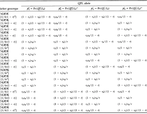
TABLE 1

Conditional probability of QTL allele given flanking (fully informative) marker genotypes

QTL allele

Marker genotype

f i

= Pr(QlI,)

fi

= Pr(QlI,)'

pi,

= Pr(

@

I

1,) = Pr(@I"

Frequencies are shown in brackets.

a Note that f i j = 1 -

pij

for s = m, J:

words, l7and A themselves are considered as random vari-

ables with their own distributions. Therefore, the above Equa-

tion 2 is a conditional likelihood function. The full likelihood

function must incorporate the distribution of (HA). Thus, the

main theme of developing the full likelihood function is to

develop the joint distribution of (nA) using marker informa-

tion.

Fully informative markers: A fully informative marker is one where all four alleles in the parents are distinguishable

APB;"/A,"E and A{B(/A4&H

from each other, i.e., the arental marker genotypes are

Consider a trait locus, Q, is flanked by the two markers, A and B . Let r be the recombina- tion fraction between A and B , and ?-,A or rB be the recombina- tion frequency of Q with A or B . Let AYQB;"/A,"@"G and

A f @ B ( / A J & & be the genotypes of the male and female parents, respectively. Here, I have assumed that markers are fully informative and the parental linkage phases are known.

In the offspring pool, there are 16 possible genotype classes

for the two flanking markers and four possible genotypes for the QTL (see Table 1 ) . Let

p:

= Pr ( Q

I

IM) be the probability that j has received allele Q conditional on information of

the marker genotypes (Z,). Then the probability that j re-

ceives Q must be &; = Pr(

@'I

I,) = 1 -

p:.

Similarly, let

dj

= Pr( @

I

I , ) be the corresponding probability that the jth

offspring receives allele @, and consequently

hj

=

Pr( @

I

I,) = 1 - prj is the probability that allele @ passes to

individual j . These conditional probabilities are listed in Ta- ble l . The table lists four conditional probabilities, each corre- sponding to the probability that an individual receives an allele from one of its grandparents. These conditional proba-

bilities are fundamental to the computation of the joint distri-

bution of the alleles IBD shared by siblings.

Marginal distributions of 7rq and 8,: The IBD proportion shared by i a n d j , 7ry, can take one of three values, as described

below:

1. 7ry = 0 if i and j receive no common alleles from their parents. This has a probability of

p ,

= Pr(7rij = 0) = [pli(l -

f,;)

+

py(1

- p;l)]

X [&i(l - &I)

+

&,(I -

& J I .

1954

s.

xu

pl,, = Pr(.?r,- = % ) = -

fl)

+

pi^ -

b7)l

X

[p{ip{j

+ (1 -

p{J)(l

-

~ { J I

+ [P-fi(l -

pij)

+

p{j(l -

pTi)I[pZfl

+

(1 -

b7)(1

-

p;t)I.

3. rq = 1 if i and j receive common alleles from both their parents. The probability is

pl = Pr(r, = 1) =

[hip:

+

( 1 - ply)(l -

pZ)l

X

[p$tp{l

+

(1 - P 4 j ) ( 1 -

piJI.

In the event that i and j receive both alleles IBD, Oq can take values of 1 and 0, with probabilities Pr(0, = 1) = and Pr(6, = 0 ) = 1 - f i , respectively.

Now, we can see that the distributions of r ' s and 0's are fully specified by the conditional probabilities,

ply

and

p{?

In summary, the marginal distributions of r q and Oq are

I

0 with probability

po

T , = with probability

pl,,

1 with probability

pl

and

@,=

[

1

with

probability

p ,

0 with probability 1 -

p , ,

respectively.

Joint distribution of (llA}: At the point (position Q) of the tested chromosome, we define two indicator variables for indi-

vidualj, %and wJ. Ifjreceives @from the male parent, define

+ =

1, which has a probability

p;,

otherwise, zl = 0. Similarly, if j receives Q{ from the female parent, define w i = 1, which has a probability of

p{j,

otherwise, wj = 0. The IBD proportion between iandjis then expressed as a function of the indicator variables,

r q = {[ZiZJ+ (1 - % ) ( l - 5 ) l

+

[WiWj+ (1 - w A ( 1 - Wj)ll/2

Oq

= [z&

+

( 1 - z;)(1 - 5)][W,Wj

+

(1 - W i ) ( l - Wj)].

and

II

and A have been expressed as functions of z = [zl Q *

-

* a ]

and w = [wl y * * .w,,]~, i.e., ll = l l ( z w) and A = A(z w).

Conditional on

p

4

and

p{j,

these indicator variables are inde- pendent, each with a Bernoulli distribution. Therefore, the joint distribution of (z w) is

R ( z w) =

n

( P r ; ) Z l ( l - f i T ) 1 - Z j ( p $ ) y l -

p4j)l-Y

(3)

j= 1

Subsequently, the joint distribution F(ll A ) is derived from

R(z w), as shown below,

F(ll A) = R(z w) (4) z € n w € g

where R and ((I are the spaces where z and w, respectively,

take their values to generate ll and A. The explicit form of

the joint distribution (Equation 4) is not required when the full likelihood function is computed because it is expressed as function of the joint distribution of z and w.

Expectations and variances

of

rq and 8,: Having been ex- pressed as a function of the Bernoulli variables, the expecta- tions, variances and covariances of r q a n d Ovare easily derived.

First, let us consider the expectations and variances of q and

zq.

Since zj and wj are independent Bernoulli variables, we

have

E ( % ) = 6 9

Var(%) =

pYy

-

p;),

Var(wJ) =

p{j(l

-

E ( Y ) =

p$J,

and all covariances are zero. We now have

E(.ir,) = ( [ E ( W ( 5 )

+

(1 - E(z,))(l - E(%))]

+

[E(wi)E(wJ)

+

( 1 - E(wi))(l - E(wj))11/2

= (#

+

6,)/2,

X [E(wz)E(wj)

+

(1 - E(wz))(l - E ( q ) ) I

#6,,

E ( @ q ) = [ E ( & ) E b j )

+

(1 - E(%))(1 - E(z,))l

where

#

=

&a;;

+ (1 - p;)(1 -

6,

is the probability that i and j share a common allele from

their father, and

6,

=

pQ4,

+

(1 - f4])(1 - Hi)

is the probability that they share a common allele from their

mother.

After some algebraic manipulation, we have

Var(r.,) = - #)

+

q{(1 - q$)l/4,

Var(@,) = gqg1 -

#&.

The covariances are

Cov(rq, r t k ) =

[(Gk

-

&&)

+ ( 6 , k - 6,dk)k)l/4,

cov(@y, 0 t h ) = # k d k -

#&d$,

Cov(.ir,, 0,) = -

G)

+

#q$1 - 6,)1/2

Cov(rij, 0th) = [ # k d k

+

6 , k & - @&(6,

+

& ) 1 / 2 9

where

#k = fi?fiifimk f ( 1 -

p;f)

( l -

p;")

( l - fimk)

is the probability that i , j and k share a common allele from their father, and

q { k =

p i i d f l i k

+

(1 -

p{j)

( l -

p{i) ( l

- p { k )

is the probability that the three sibs share a common allele from their mother.

Partially informative markers: Any marker loci with three or less distinguishable alleles in the parents is considered to be partially informative or noninformative. There is a simple method to construct the conditional probability table based on information provided by Table 1. If an allele is indistin- guishable from another, one must combine the indistinguish-

able genotype classes (see Table 1) together to obtain the

corresponding

Pr;

and

Prj.

The combined fi;f and

f4,

are the weighted averages of those conditional probabilities with the

marker genotypic frequencies (bracketed in column one of

Table 1 ) being the weights. For example, if B;" =

E,

marker genotypes AT&B;&E and AT&E€$ are indistinguishable, and thus should be combined. The combined genotype class has

p;;

= [%(l - r ) ,

+

%r(l - r)]"

x [%(I - r)'(1 - T A ) ( 1 - T B )

+

(1 - r )

+

- r ) ( l - rA)rB/r]

and

If both markers are noninformative, all 16 classes of marker genotype should be combined and weighted by the frequen- cies (see column 1 of Table 1). In this case, all conditional probabilities

(pi:

and

pi,

for all j s ) are

x,

which is exactly what we would have anticipated. In real data analysis, if a marker is not informative, one should replace it by a nearby but informative (or partially informative) marker.

When the parental linkage phases are unknown, all four possible mating types should be considered,

and

A table listing

p;”,

and

p i j

should be generated under each possible linkage phase and the overall

pi

and

p i j

are the averages of the four phase-specific conditional probabilities

weighted by the prior probabilities of the four types of linkage

phase.

Full likelihood function: Given the fact that ll and A are random variables, there are two ways to implement the likeli- hood function. The usual practice is to construct the likeli-

hood function with lland A replaced by their expectations

(GOLDGAR 1990). The likelihood function built in such a way is denoted by

L E = U P l y

“1,

(5)

and the method will be referred to as the “expectation

method.” This likelihood function is not the full likelihood function because it does not use the joint distribution of (Il

The full likelihood function is to be established by using the joint distribution of ll and A. It is essentially an average of likelihoods evaluated at all possible values of ll and A,

weighted by their probabilities (SCHORK 1993). The full likeli- hood function is expressed by

L

= W l y l =

Z

J W I Y

n A l f l n A )

4 .

na

= U P l y w)A(z w)l@ w) (6)

ZUI

and will be referred to as the “distribution method.”

Recall that each one of z’s and w’s takes one of two possible

values, 0 and 1, and the total number of summations is 4”.

The summation will quickly become computationally prohibi-

tive as the number of sibs increases. For example, 4“ =

1048576 when n = 10. Therefore, the distribution method implemented this way is practical only for small families, as in human populations. For large families, special algorithms,

such as the Monte Carlo algorithm, may be used, which will

be discussed later.

AN ILLUSTRATION

To illustrate the procedure, I use a full-sib family of five members that come from a fully informative mating

type A1Bl/A2& X A,&/4B4 as an example. Here, I

assume that the distance between marker A and B is 20

cM ( r = 0.1648) and the QTL is right in the middle of

the interval (rA = rB = 0.0906). Table 2 lists the geno-

types of markers, phenotypic values and conditional

probabilities of QTL alleles of the five sibs.

Expectations, variances and covariances: Computa- tion of the conditional expectations, variances and covari-

ances of the IBD proportions between sibs 2 and 4 ( x 2 4

and Oz4) will be demonstrated in details. The IBD propor-

tions between sibs 2 and 3 (x23 and 0 2 3 ) will be investi-

gated in regard to their covariances with x 2 4 and

OZ4.

If individuals 2 and 4 receive no common alleles from

their parents, then x 2 4 = 0 , which has a probability

p,

=

[ p w

- pY4)

+

p w

- f l Z ) l [ H 2 ( 1 - H 4 )

+

H4(l

-

Hz)]

= 0.4903.

If sibs 2 and 4 receive a common allele from their father

but different alleles from their mother or they receive a common allele from the mother but different alleles

from the father, then x 2 4 =

%

with a probability

p1/2 = [ f l Z ( l - f l 4 )

+

pZ(1

- f l 2 ) I [&2pf4

+

(1 - H4)

x

(1 -

& d l

+

[ & 2 U - H 4 )

+

& 4 ( 1 -

&,)I

X [pEfim4

+

(1 -

P;;)]

= 0.5.

Finally, if the two sibs receive common alleles from both

of their parents, then x 2 4 = 1 with a probability

fi

= iflZfl4

+

( 1 - p 7 4 ) (1 -

p;”,)]

x

[p$2p’f4

+

(1 - p 4 4 ) (1 -

p i e ) ]

= 0.0097.

The distribution of $24 is simply $24 = 1 with probabil-

ity

pl

= 0.0097 and

OZ4

= 0 with probability 1 -

pl

=

0.9903.

In summary, the marginal distributions of x 2 4 and

OZ4

are

0 with probability

p,

= 0.4903

with probability

pl,2

= 0.5000

1 with probability

fi

= 0.0097

and

{

1 0 with probability with probability

p,

1 - = pl 0.0097 = 0.9903,

0 2 4 =

respectively.

ances are easily computed, as shown below,

1956

s.

xu

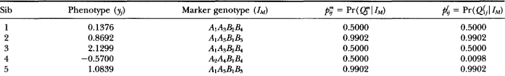
TABLE 2

Phenotypic values, marker genotypes and conditional probabilities of QTL alleles of the five sibs given in the example (mating type = A,B,/A& X A&/A&)

Sib Phenotype (yj) Marker genotype (Z,)

p;

=

Wgl

ZM)

6,

= W Q f j l Z M )

1 0.1376 AIA3&B4 0.5000 0.5000

2 0.8692 AI&&& 0.9902 0.9902

3 2.1299 AtAs&B4 0.5000 0.5000

4 -0.5700 Az%BIB~ 0.5000 0.0098

5 1.0839 AIA~BIB, 0.9902 0.9902

E(r24) =

pl

+

o.5p1/Z = 0.2597 and

E(6’24) = = 0.0097.

Consider

6 4 = p?2$4

+

(1 - f l 4 ) ( l - f l 2 )

= 0.9902 X 0.5

+

(1 - 0.9902) (1 - 0.5) = 0.5

and

4 4 = dZd4

+

( l

-

d4) ( l -

d2)

= 0.9902 X 0.0098

+

(1 - 0.9902) (1 - 0.0098)

= 0.0194,

we have the variances

Var(rz4) = [&(I - &)

+

& ( I - d4)1/4

= [0.5(1 - 0.5)

+

0.0194(1 - 0.0194)]/4 = 0.0673

and

~ar(O24) = @444(1 - @4&)

= 0.5 X 0.0194 X (1

-

0.5 X 0.0194) = 0.0096.

We need the following additional quantities to com- pute the covariances,

$3 =

pr;p;”s

+

(1 -

p3)

(1

-

p 3

= 0.9902 X 0.5

+

(1 - 0.9902) (1 - 0.5) = 0.5,

43

= d2d3

+

(1 -

H3)

(l - H Z )

= 0.9902 X 0.5

+

(1 - 0.9902) (1 - 0.5) = 0.5,

&4 =

p?@Gp?4

+

(1 -

p;)

-

p;)

(l - $4)

= 0.9902 X 0.5 X 0.5

+

(1 - 0.9902) (1 - 0.5) (1 - 0.5) = 0.25

and

4 3 4 = dZd3H4

+

(1 -

HZ)

(l - $43) (l -

d‘l)

= 0.9902 X 0.5 X 0.0098

+

(1 - 0.9902)

(1 - 0.5) (1 - 0.0098) = 0.0097.

Given the above quantities, the following covariances are computed,

cov(rz3, r z 4 ) = [ ( & 4

-

&&)

( 4 3 4 - &44)1/4

= [(0.25

-

0.5 X 0.5)

+

(0.0097

-

0.5 X 0.0194)]/4 = 0.0,

c o v ( ~ 2 3 ~ O24) = & 4 4 3 4

-

6 3 @ 4 4 3 4 4

= 0.25 X 0.0097

- 0.5 X 0.5 X 0.5 X 0.0194 = 0.0,

cov(r24, O 2 4 ) = [644q44(1 - 6 4 )

+

@4d4(1 -

qi4)1/2

= [0.5 X 0.0194 X (1 - 0.5)

+

0.5 X 0.0194 (1 - 0.0194)]/2

= 0.0072,

c o V ( r z 3 , 6 ’ 2 4 ) = [@3444 434@4 - @ 4 4 4 ( &

+

@3)I/2

= [0.25 X 0.0194

+

0.0097 X 0.5

- 0.5 X 0.0194 X (0.5

+

0.5)]/2

= 0.00485.

Likelihood function: With a single family of five sibs, we may not have meaningful maximum likelihood esti- mates of the unknown parameters, but given the para- metric values, we can evaluate the likelihood function.

I assume that /..L = 0 , 0; = 1.0, 0; = 0.25, 0; = 0 and

a:

= 1.25.

The expected

ll

and

A

are

-

1 0.5 0.5 0.5 0.5

0.5 1 0.5 0.2597 0.9806

E(n)

= 0.5 0.5 1 0.5 0.5

0.5 0.2597 0.5 1 0.2597

-

0.5 0.9806 0.5 0.2597 1

and

-

1 0.25 0.25 0.25 0.25

0.25 1 0.25 0.0097 0.9616

E(A)

= 0.25 0.25 1 0.25 0.25

0.25 0.0097 0.25 1 0.0097

Substituting E ( l 7 ) and

E(A)

into (5), we have I& =

0.0003794 and the natural log of L); is In(L):) =

The likelihood function evaluated using the distribu-

tion method (Equation 6) is LI) = 0.0003799 with a

natural log being In(Ln) = -7.8756.

In this particular example, the likelihood values of the two methods show very little difference, but the difference will vary from family to family and the differ- ences cumulate as the number of families increases. Factors that influence the difference include the QTL

variances

(a:

and o:), the information content of the

flanking markers and the distance between the QTL and the markers. The difference is expected to increase as the QTL variances increase and/or the distance be-

tween the QTL and the markers increases. It is expected

to decrease as the markers become more informative. The information content of the markers and the QTL

position determine the deviations of

pyj

and

dj

from

fr,. The more the

p;

and deviate from

1,

the less the

uncertainty (variance) of the IBD proportion and the

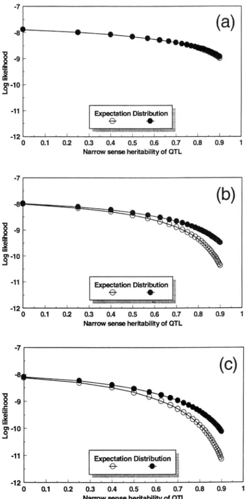
smaller the difference between the expectation and dis- tribution methods. This can be shown in the following example. Consider the phenotypic values of the five

sibs listed in Table 2. Let the additive QTL variance vary

and all other parameters be fixed at their previously

designed values ( p =

0,

a:

= 0.25, a: =

0

and af =

1.25). Let o i vary between 0 to 13.5 so that the narrow

sense heritability of the QTL varies between 0 and 0.90.

We will examine three situations with regard to the

deviations of pGand

p { j

from 0.5: (1) extreme deviation,

i.e.,

p5

= ~j = 0.99 for a l l j (2) intermediate deviation,

i.e.,

p;l)

=

d j

= 0.85 for all

j

and (3) no deviation, i e . ,

p t

= PCj = for allj. The likelihood functions evaluated

using the two methods (expectation and distribution) are computed under each of the three situations. The

results are depicted in Figure 1 , which verifies our pre-

diction.

-7.8769.

DISCUSSION

I have demonstrated that

l7

can be expressed as a

function of z and w (see definitions of z and w). Because

z and w are independent Bernoulli variables, the joint

distribution of

l7

is easily derived. The likelihood func-

tion was built in two ways: (1) replacing

l7

by its expecta-

tion (the expectation method) and (2) using the joint

distribution of

l7

(the distribution method). I now in-

vestigate the difference between the two methods from

a more theoretical point of view. Let L = f(z, w) be the

conditional likelihood function, expressed as function

of z and wand evaluated at true value of

0.

We can see

that likelihood function of the expectation method is

LE = f [ E ( z ) , E W l

and that of the distribution method is

L,, =

4 1 .

4 1

-1 2

0 0.1 0 2 0.3 0.4 0.5 0.6 0.7 0.8 0.9 Narrow sense heritability ot QTL

I

I

-1 2

0 0.1 0 2 0.3 0.4 0.5 0.6 0.7 0.8 0.9 1

s eheritawity ~ ot

a n

-1 2

0 0.1 0.2 0.3 0.4 0.5 0.6 0.7 0.8 0.9 1

N.-W ~enm hema~rty of

a n

FIGURE 1.-Log likelihood values of the expectation ( 0 )

and distribution ( 0 ) methods for the phenotypic data of the five sibs given in the example. The likelihood function of the expectation method is obtained by replacing the unknown IBD proportions by their expected values while that of the distribution method is obtained by incorporating the distribu- tion of the unknown IBDs. Three situations are examined based on the uncertainty of the IBD proportions: (a) IRDs are almost known without error, (b) the IBDs are partially known with intermediate uncertainty, and (c) the IBDs are completely unknown. Narrow sense heritability is the ratio of the additive QTL variance to the total phenotypic variance.

In other words, the expectation method uses the func-

tion of the expectation as the likelihood, whereas the

distribution method uses the expectation of the func-

1958

s.

x u

LD is due to nonlinearity off(z, w) with respect to z and w. If f(z, w) were linear, LE and Lo would be identical. Therefore, LE is the first order approximation of Lo at point (E(z)E(w)}. Let u = [z"w'] a ( 2 n )

x

1 vector, then L can be expressed by Taylor expansions around the expectation of u,

L = f[E(u)]

+

[u -

X -

dU&"

a'(u) [u - E(u) ]

+

higher orders,

where the first and second partial derivatives are evalu- ated at E(u). Ignoring higher order terms and noting

E[u - E(u)] = 0, we have

Since elements of u are independent, conditional on

p:

and

hj,

the above equation can be simplified as

Lo

=

LE

+

E ,

where

Therefore, the expected difference between Lo and LE

is approximately equal to E . Since the second partial

derivatives are always nonnegative, E 2 0, implying LD 2 LE. Under the null hypothesis H,, 0; = 0: = 0 , L,,

= LE, but under H A , ui f 0 and u: z 0, Lo 2 LE. We then conclude that the power of the distribution method is never smaller than that of the expectation method. The above conclusion is only approximate, but will hold in most situations.

Lander and Botstein's (1989) interval mapping uses the full likelihood function and thus is the distribution method, though under the fixed model. Haley and Knott's (1992) simple regression method implicitly uses the expectation method (replacing the QTL genotype indicator variable by its conditional expectation). In line crossing experiments, every polymorphic marker is fully informative, thus when the QTL is located at a marker locus, the two methods are identical. The difference between the expectation and distribution methods is expected to increase when the QTL is fur- ther away from either flanking marker. These conclu- sions also hold in the comparison of the two methods under the random model approach. In human popula- tions, however, many marker loci may be partially infor- mative. Even if the QTL resides exactly at a marker locus, the expectation method may still differ from the distribution method because Var(zj) and Var(w,) may not be zero if the marker is not fully informative.

The distribution method is computationally more de- manding than the expectation method, but it is man- ageable in human populations because family sizes are typically small. In animal or plant populations where the family sizes are usually large, efficient algorithms and computer programs must be used. Here I show how a Monte Carlo algorithm can be used to evaluate the full likelihood function. It is simple and intuitive, though other algorithms are also available. Since

5

and wl follow Bernoulli distributions with parameters

p5

and

hj,

respectively, they can be generated via Monte Carlo simulation. Let Z, and W, be the ah realizations of vectors z and w, then the full likelihood function can be approximated by

l M

LIl= L[Plyl

=

-

c

L [ P l y

n(ztW,)A(ztw,,I,

t = l

where M is typically in the order of 1000. Although M

does not need to increase as the family size increases, the computation is still impractical for very large fami- lies because repeated matrix inversion is required. In such as case, rather than using the full maximum likeli- hood method, a Bayesian approach via the Gibbs sam- pling method may be more efficient (GEMAN and GE-

MAN 1984; GELFAND and SMITH 1990). This is beyond

the scope of this paper, and thus is not further dis- cussed.

Throughout this paper, I have assumed that there is no inbreeding, i e . , parents are genetically unrelated. Mild inbreeding may be ignored without having serious impact on the results. For example, if there are 50 fami- lies each with a few sibs, a couple of inbred families

(e.g., mating between cousins) is not likely to distort the theory. In animal and plant populations, however, inbreeding is common and may not be ignored. The procedure developed in this paper can be extended to cover inbreeding families. Here, I consider a special example of inbreeding, i.e., selfing. A general proce- dure that covers arbitrarily inbred families may be de- rived following the framework of this example. Recall that there are four alleles contributing to the family, which are

G,

am,

@, @,

and there are four possible genotypes:

GQf,

QJ"@,

am@

and

@@.

Under selfing, the male and female parents are identical, therefore, QJ

=

and @'

=

@,

where the symbol represents identical by descent. Whenever an individual has a ge- notype

am@

or

am@

it is inbred. Thus, the probability of individual j being inbred is

pGp(J

+

( 1 -

PC)

(1 -

pfJ.

The diagonal elements of

Il

must be modified to

take into account the possibility of inbreeding. Ex- pressed as a function of zi and wI, the jth diagonal ele- ment of

n

is

7rJ = 1

+

$Wl

+

(1 - Z , ) ( l - Wj)

E(7r,) = 1

+

p;p4,

+

(1 -

p;",,

(1 - $4,).

The offdiagonal elements of

n

must be modified ac- cordingly, as given below

7rij = ([z&

+

( 1 - Z j ) ( l - zj)]

+

[UiU,

+

(1 - Ui)

x

(1 - w,)l

+

[ZiW,

+

(1 - % ) ( I -

q ) l

+

[WiZ,

+

(1 - W A ( 1 - z,)ll/2,

with an expectation of

Qnq) = (Qz;

+

6,

+

qyf

+

&)/2,

where

qyf

=

p;tp$

+

(1 -

fiy)

(1 -

p f , )

and

&

=

There are two important issues in QTL analyses that deserve further discussion. One is the sampling strategy and the other is the statistical methodology. It is well known that using data sampled from offspring of hy- brids initiated from diverged homozygous lines is very powerful. Statistical methods of genetic mapping in line crosses are well documented

(e.g.,

LANDER and

BOTSTEIN 1989; HALEY and KNOTT 1992; JANSEN 1993;

ZENG 1994). Using data generated from such designed

experiments, these authors know exactly how many al- leles at the putative QTL (two alleles at most), the fre- quency of each QTL allele (0.50 at each segregating locus), and in most situations, the linkage phases. As a result, they can unambiguously estimate the effect of allelic substitution at a putative position of the genome. After QTL are located in the genome and their effects are estimated, the segregation variance of each QTL can be computed based on the estimated effect and the known allelic frequency. What are actually reported in the literature are not the effects (first moments) but the variances (second moments) relative to the total phenotypic variance in the segregating populations. These QTL variances, however, may have limited uses. Because of the sampling nature, the QTL variances do not represent the actual variation occurring in natural populations and the statistical inference is limited to the two parental lines.

When mapping QTL in natural populations, we no longer enjoy the luxury of knowing the number of al- leles and the allelic frequencies of putative QTL and thus some power must be sacrificed. What we gain by using natural populations is a broad statistical inference space. Namely, the estimated QTL variances may reflect the actual variation existing in the population where the experimental units are sampled.

Under the assumption of finite alleles per locus, Els- ton and Stewart (1971) developed a general algorithm to compute the full likelihood function for extended pedigrees. Morton and McLean (1974) gave an efficient algorithm for independent full-sib families. This algo- rithm was recently rediscovered by Knott and Haley (1992) who applied it for mapping QTL using indepen- dent full-sib families. Although the number of alleles is not known in general, biallelic model is normally as-

piip;S.

+

(1 - ~ j(1 )-

p;).

sumed

(mom

and HALEY 1992). Multiple alleles can be easily taken into account and the full likelihood function can be obtained by summing up the condi- tional likelihoods for all possible genotypes weighted by the genotypic frequencies (ELSTON and STEWART 1971). The model presented by these authors is commonly recognized as discrete model because the QTL effect in the sampled population does not have a continuous distribution. In contrast, the model presently in this paper may be referred to as continuous model because the QTL effect is assumed to have a normal distribution. There is no simple answer to the question of which model is closer to reality. If the referenced population is the sample, the total number of alleles is always finite, thus the discrete model is the choice. If, however, the referenced population is the overall population where the sampled pedigrees are drawn, neither model is ex- act because the number of alleles in the overall popula- tion is rarely known. However, the normal distribution of the allelic effects is usually a very robust assumption. This has been verified by Xu and Atchley (1995) who analyzed simulated data generated from a biallelic rather than normal distribution and found dramatic agreement between the estimated and the true vari- ances. The continuous model approach has been exten- sively investigated for linkage analysis by researchers in the field of animal genetics (e.g., FERNANDO and GROSS- MAN 1989; GODDARD 1992; GRIGNOLA et al. 1994; VAN

ARENDONK et al. 1993, 1994; WANG et al. 1995), either explicitly or implicitly using the conditional expecta- tions rather than the distributions of the IBDs.

In conclusion, I provide a general method to com- pute the full likelihood function for estimating the vari- ance at a QTL using marker information. I also show that the distribution method is at least as powerful as the expectation method, which is consistent with the sib-pair analysis conducted by Kruglyak and Lander (1995). Although increase in power and efficiency of

the distribution relative to the expectation method is achieved at the price of low speed of computation, given the availability of high speed computers, one should be concerned more about the power and efficiency than the computing speed. Especially, when markers are not fully informative and have a low density in the genetic maps, power increase can be substantial.

Comments from two anonymous reviewers helped the author clar-

ify some ambiguities in an early version of the manuscript and thus are very much appreciated. I also thank DAMIAN GESSLER for his helpful comments. This research was supported in part by National Research Institute Competitive Grants Program/USDA 95-37205- 2313.

LITERATURE CITED

CARDON, L. R., S. D. SMITH, D. W. FULKER, W.J. KIMBERLING, B. F. PENNINGTON et al., 1994 Quantitative trait locus for reading disability on chromosome 6. Science 266: 276-279.

1960

s.

x u

FERNANDO, R. L., and M. GROSSMAN, 1989 Marker assisted selection using best linear unbiased prediction. Genet. Sel. Evol. 21: 467- 477.

FULKER, D. W., and L. R. CARDON, 1994 A sib-pair approach to inter- val mapping of quantitative trait loci. Am. J. Hum. Genet. 54:

GELFAND, A. E., and A. F. M. SMITH, 1990 Sampling-based a p proaches to calculating marginal densities. J. Am. Stat. Assoc. 85:

GEMAN, S., and D. GEMAN, 1984 Stochastic relaxation, Gibbs distri- butions and Bayesian restoration of images. IEEE Trans Pattern Anal Machine Intelligence 6: 721-741.

GODDARD, M., 1992 A mixed model for analyses of data on multiple genetic markers. Theor. Appl. Genet. 8 3 878-886.

GOLDGAR, D. E., 1990 Multipoint analysis of human quantitative ge- netic variation. Am. J. Hum. Genet. 47: 957-967.

GRIGNOLA, F. E., I. HOESCHELE and K. MEYER, 1994 Empirical best linear unbiased prediction to map QTL. Proc. 5th World Congr. Genet. Appl. Livestock Production 21: 245-248.

HALEY, C. S., and S. A. KNOTT, 1992 A simple regression method for mapping quantitative trait loci in line crosses using flanking markers. Heredity 69: 315-324.

HASEMAN, J. IC, and R. C. ELSTON, 1972 The investigation of linkage between a quantitative trait and a marker locus. Behav. Genet.

JANSEN, R. C., 1993 Interval mapping of multiple quantitative trait loci. Genetics 135: 205-211.

JIANG, C., and Z.-B. ZENG, 1995 Multiple trait analysis of genetic mapping for quantitative trait loci. Genetics 140: 11 11

-

1127. W o n , S. A,, and C. S. HALEY, 1992 Maximum likelihood mapping

of quantitative trait loci using full-sib families. Genetics 132: 1211-1222.

1092-1103.

398-409.

2: 3-19.

KRUGLYAK, L., and E. S. LANDER, 1995 Complete multipoint sib-pair analysis of qualitative and quantitative traits. Am. J. Hum. Genet.

57: 439-454.

LANDER, E. S., and D. BOTSTEIN, 1989 Mapping Mendelian factors underlying quantitative traits using RFLP linkage maps. Genetics

121: 185-199.

MORTON, N. E., and C. J. MCLEAN, 1974 Analysis of family resem- blance. 111. Complex segregation of quantitative traits. Am. J. Hum. Genet. 2 6 489-503.

OLSON, J. M., 1995 Robust multipoint linkage analysis: an extension of the Haseman-Elston method. Genet. Epidemiol. 12: 177-193.

SCHORK, N. J., 1993 Extended multipoint identity-by-descent analy- sis of human quantitative traits: efficiency, power, and modeling considerations. Am. J. Hum. Genet. 5 3 1306-1319.

VAN ARENDONK, J. A. M., B. TIER and B. P. KINGHORN, 1994 Simulta- neous estimation of effects of unlinked markers and polygenes on a trait showing quantitative genetic variation, p. 192 in Pro- ceedings 17th International Congress of Genetics, Birmingham,

UK.

VAN ARENDONK, J. A. M., B. TIER and B. P. KINGHORN, 1993 Use of multiple genetic markers in prediction of breeding values. Genetics 137: 319-329.

WAN(;, T., R. L. FERNANDO, S. VAN DER BEEK, M., GROSSMAN and J. A. M. ARENDONK, 1995 Covariance between relatives for a marked quantitative trait locus. Genet. Sel. Evol. 27: 251-274.

Xu, S., and W. R. ATCHLEY, 1995 A random model approach to interval mapping of quantitative trait loci. Genetics 141: 1189- 1197.

ZENG, Z.-B., 1994 Precision mapping ofquantitative trait loci. Genet- ics 136: 1457-1468.