STOCHASTIC SITE RESPONSE ANALYSIS THROUGH UNCERTAIN
ELASTOPLASTIC SOIL
Fangbo Wang1, Hexiang Wang2, Han Yang2, Yuan Feng3, Boris Jeremić4,5
1Assistant Professor, Tianjin University, Tianjin, China
2PhD Candidate, University of California, Davis, CA, USA
3Research Scientist, TuSimple, San Diego, CA, USA
4Professor, University of California, Davis, CA, USA
5Faculty Scientist, Lawrence Berkeley National Laboratory, Berkeley, CA, USA
ABSTRACT
Presented is a stochastic site response analysis with uncertain seismic motion and uncertain elastoplastic
material. The uncertain soil parameters and seismic motion are modelled as random fields and random
process, and both represented by Hermite polynomial chaos. The site response, also represented by Hermite
polynomial chaos, is solved for following a developed intrusive stochastic finite element formulation based on
stochastic Galerkin method. Risk implications from the analysis are also discussed. Presented methodology
is implemented in the Real ESSI Simulator system.
INTRODUCTION
A site response analysis, i.e., determines the response of soil deposit from the input bedrock motion,
is able to predict ground surface motions, to evaluate soil dynamic stress and strains, and to assess the
stability of earth-retaining structures. Material parameters and input motions of conventional site response
analysis [3] are mostly deterministic. However, due to limited data, spatial non-uniformity of soil has been
long recognized by civil engineering community and soil parameters are considered to be uncertain [4]. In
addition, uncertainties of seismic motion arises from the seismic source, wave propagation path, etc. Also,
it is computationally challenging to consider the uncertainties in the structural system.
Among the available numerical techniques, Monte Carlo method [5] is the most commonly used approach.
It repeatedly calls the deterministic solver with generated samples of uncertain parameters. Statistics of
structural response maybe post-processed after collecting results from all sample runs. However, Monte
Carlo method is notorious for slow convergence and requires a large number of samples to reach acceptable
accuracy but computationally intractable. In this paper, Hermite polynomial chaos is employed to represent
the uncertainties of material parameters and seismic motion, and a time-domain stochastic dynamic finite
element formulation is employed to propagate the input uncertainties through the soil deposit. We will first
present the stochastic dynamic finite element formulation, and the probabilistic constitutive model of soil. A
stochastic site response analysis with uncertain soil deposit and bedrock motion will be conducted using the
Division III
STOCHASTIC DYNAMIC FINITE ELEMENT FORMULATION
In the developed time domain stochastic Galerkin formulation, uncertain material parameters and forcing
are simulated as non-Gaussian random fields and stationary/non-stationary random process, which can be
quantified by Hermite polynomial chaos (PC) expansion. In addition, the response processes, displacement,
acceleration, are also represented with Hermite PC. Then, stochastic Galerkin projection is applied to
minimize the error on estimating response PC coefficients. The statistics and distributions of displacement,
acceleration maybe post-processed for design and risk analysis purposes.
Hermite PC representation of random process
The weak form of deterministic, dynamic finite elements [2] can be written as:
Z
De
Nm(x)ρ(x)Nn(x)dΩu¨n(t)+
Z
De
∇Nm(x)D(x)∇Nn(x)dΩun(t)− fm(t) =0 (1)
whereNmis the finite element shape function,Ωand fm(t)incorporates the various elemental contributions to the global force vector.
Next, we assume the (tangent) stiffness, D(x), and the forcing function, fm(t), to be a heterogeneous random field and a non-stationary random process, respectively and represent them in terms of
multidimen-sional, Hermite PC expansions with known coefficients. Details of Hermite polynomial chaos quantification
of random field/process can be found in [6, 7].
D(x, θ)=
P1
X
i=1
ai(x)Ψi({ξr(θ)}) (2)
fm(t, θ)= P2
X
j=1
fm j(t)Ψj({ξr(θ)}) (3)
where P1 = (M1 +p1)!/(M1!p1!) and{Ψi} are multidimensional, orthogonal and uncorrelated, Hermite polynomials of zero-mean, unit variance Gaussian random variables,{ξr}, while M1andp1are the
corre-sponding dimension and order in the PC representation. Note that θ is introduced to denote uncertainty.
Similarly, P2 = (M2+p2)!/(M2!p2!). As a result, the nodal displacement, un(t), and nodal acceleration, ¨
un(t), will also become random processes. They will also be represented using multidimensional, Hermite
PC expansions but with unknown coefficients which will be computed using a stochastic Galerkin approach.
Stochastic Galerkin approach to compute PC coefficients of displacement, acceleration response processes
The PC representation of response process should include all the input uncertainties, therefore, the PC
nodal displacement,un(t), in terms of a multidimensional Hermite PC expansion of dimensionM1+M2and
orderQas:
un(t, θ) = P3
X
k=1
dnk(t)Ψk({ξl(θ)}) (4)
whereP3 = (M1+ M2+Q)!/((M1+M2)!Q!). Twice differentiating Eq. 4, we obtain a multidimensional
Hermite PC representation of nodal acceleration, ¨un(t), as:
¨
un(t, θ) = P3
X
k=1
¨
dnk(t)Ψk({ξl(θ)}) (5)
Substitute Eqs. 2, 3, 4, and 5 into Eq. 1, and denote the shape function gradients∇Nn(x)asB(x), we obtain
P3
X
k=1
Z
De
Nm(x)ρ(x)Nn(x)dΩ Ψkd¨nk(t) +
P3
X
k=1 P1
X
i=1
Z
De
Bm(x)ai(x)Bn(x)dΩ ΨiΨkdnk(t)− P2
X
j=1
fm j(t)Ψj =0
(6)
Multiplying both sides of Eq. 6 byΨl and taking ensemble average, namely stochastic Galerkin projection
[1], we obtain the following system of ordinary differential equations:
P3
X
k=1 hΨkΨli
Z
De
Nm(x)ρ(x)Nn(x)dΩ d¨nk(t) +
P3
X
k=1 P1
X
i=1
hΨiΨkΨli
Z
De
Bm(x)ai(x)Bn(x)dΩ dnk(t)= P2
X
j=1
hΨjΨlifm j(t)
(7)
withl = 1,2, ...,P3 andm= 1,2, ...,N whereN is the number of finite element nodes. Note that Eq. 7 is
identical to the deterministic finite element system of equations whenP1,P2, P3are equal to 1. Transform
Eq. 7 into matrix-vector form:
Md¨+Kd=F (8)
whereMandK may be termed as the generalized stochastic mass and stiffness matrices, whileF,d, and ¨d
may be termed as the generalized stochastic force, displacement, and acceleration vectors, respectively. Note
that the ensemble averages of the double and triple products of the PC basis functions appearing withinM, K, andFmay be pre-computed symbolically. Rayleigh damping might be added into Eq. 8, and we can get:
Md¨+Cd˙+Kd=F (9)
whereC =αM+βK, withαandβbeing the Rayleigh damping parameters. Eq. 8 or Eq. 9 may be solved
Division III
Note that the size of the stochastic finite element system of equations can be substantially larger than the
corresponding deterministic finite element system of equations, depending upon the number of PC terms
used to represent the displacement random process.
After solving Eq. 8 or Eq. 9, PC coefficients of displacement and acceleration random processes can be
substituted into Eqs. 4 and 5 to synthesize the random processes, and realizations of the processes can be
simply generated through random sampling. In addition, the evolutionary mean and standard deviation of
response processes can be computed using special properties of the PC basis functions. For example, the
evolutionary mean and standard deviation of displacement time history at nodenmay be estimated as:
µun(t)= hun(t, θ)i=dn1(t) (10)
and,
σun(t)=
v t
P3
X
k=2 hΨ2
ki(dnk(t))2 (11)
CONSTITUTIVE SIMULATION
In classical plasticity, sign of loading index is the criteria to apply elastic loading or plastic loading, i.e.,
the ’if’ condition. By assuming uncertain material parameters, the distribution of loading index would have
probability of positive loading index and probability of negative loading index at one time step, and the
distribution of stress and updated tangent modulus would be modal distributions. However,
multi-modal distributions requires Hermite PC with very high order which is impractical for computations.
In order to overcome the difficulties of ’if’ condition, the assumption of zero elastic region of material
is utilized to allow material yielding in all time steps. For a one-dimensional von-Mises material with
Armstrong-Frederick kinematic hardening, the evolution of stress can be fully represented by the back stress
of the Armstrong-Frederick hardening equation, and the incremental update of stress,∆σ, can be written as:
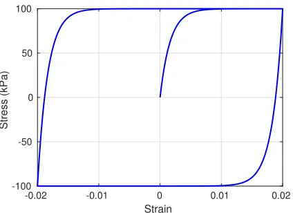
∆σ= Ha∆ −Crσ|∆| (12)
whereHaandCr are the two parameters in Armstrong-Frederick kinematic hardening rule with the material
strength to beHa/Cr. Without any loss of generality, for the case of∆ >0,
∆σ=Ha∆−Crσ∆ (13)
and the tangent stiffness can be computed as:
E = ∆σ
∆ =Ha−Crσ (14)
-0.02 -0.01 0 0.01 0.02
Strain
-100 -50 0 50 100
Stress (kPa)
Figure 1: Hysteretical stress-strain behavior of the 1-D material model withHa=60M Pa,Cr =100.
Extension to stochastic 1-D material model
The material parameters, Ha,Cr, maybe assumed uncertain with limited measurements. In addition, the
incremental strain,∆, from global level may also be uncertain. Let us representHa,Cr,∆ with Hermite
PC:
Ha = P
X
i=1
HaiΨi({ξr}) (15)
Cr = P
X
i=1
CriΨi({ξr}) (16)
∆ = P
X
i=1
∆iΨi({ξr}) (17)
σ=XP
i=1
σiΨi({ξr}) (18)
∆σ= P
X
i=1
∆σiΨi({ξr}) (19)
E =
P
X
i=1
EiΨi({ξr}) (20)
wherePis the total number PC terms in the stochastic system, andHai,Cri,∆i, σi,∆σiare corresponding
PC coefficients. Then, substitute Eqs. 15 to 20 into Eq. 13, 14, and apply stochastic Galerkin projection on
Division III
∆σi = Haj∆khΨiΨjΨki −Crlσm∆nhΨiΨlΨmΨni hΨ2
ii
(21)
Ei =Hai −
CrjσkhΨiΨjΨki
hΨ2 ii
(22)
Note that index notation is used in the above equations with index ranging from 1 to P. In addition, the
negative sign should be switched to positive if the mean of incremental strain is negative.
To illustrate the stress-strain behaviors of probabilistic constitutive model, material initial stiffness,Ha,
is assumed log-normal distribution with mean and coefficient of variation (COV) to be 60 MPa, 40%,
respectively, while strength parameter,Ha/Cr, is assumed log-normal distribution with mean and COV to be
100 kPa, 20%, respectively. Note that PC dimension 2 should be used for stress output sinceHaandHa/Cr
are two independent random variables. In addition, PC order 6 is used for the stress output. It is observed
that the stress-strain behavior from intrusive simulation is in good agreement with Monte Carlo analysis
using 10,000 samples. In addition, standard deviation of the shear strength in Figure 2 is 20%, which is the
same as input uncertainty ofHa/Cr.
-0.02 -0.01 0 0.01 0.02
Strain -150
-100 -50 0 50 100 150
Stress (kPa)
Intrusive: Mean Intrusive: Mean+/-St.Dev. MC: Mean
MC: Mean+/-St.Dev.
Figure 2: Hysteretical stress-strain behavior of 1-D material with uncertainHaandHa/Cr.
RESULTS AND ANALYSIS
By keeping the 1-D site response analysis in mind, this section presents stochastic finite element simulations
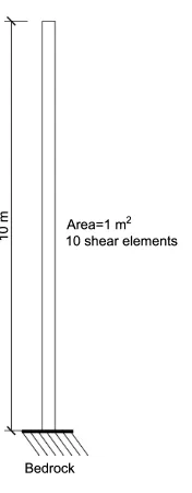
with uncertain nonlinear material parameters and bedrock motion. The soil deposit, as shown in Figure 3,
is 10 m deep and discretized into 10 shear beam elements. The material model, as formulated in previous
section, is the 1-D von-Mises model with Armstrong-Frederick kinematic hardening and zero-elastic region.
The initial stiffness,Ha, of the 1-D shear beam model is assumed to be a random field with log-normal
distribution (mean 60 MPa, COV 20%), exponential correlation structure with correlation length 10 m. We
use Hermite polynomial chaos expansion with dimension 4 order 2 to represent the random field of Ha.
The material strength parameter,Ha/Cr, is also uncertain but fully correlated with the random field ofHa.
Therefore, the marginal distribution of Ha/Cr is also log-normal but with mean 100 kPa and COV 20%.
The correlation structure of Ha/Cr is identical to that of Ha. Since we use dimension 4 for the random
E
0 Area=1 m2
T""" 1 0 shear elements
Bedrock
Figure 3: 1-D shear beam model.
acceleration, should be 154.
Uncertain bedrock motion, modelled as random process, are developed from stochastic Fourier amplitude
spectra and Fourier phase spectra. The inter-frequency correlation structure of Fourier amplitude spectrum
is captured, and the non-stationarity of ground motion is quantified by statistical phase derivative model.
Hermite polynomial chaos expansion is employed to represent the random process with the correlation
structure discretized by Karhunen-Loève expansion. For the earthquake scenario of Magnitude 7, epicenter
distance 20km, source stress drop 5MPa and site attenuate Kappa 0.02s, the statistics of the seismic motion,
marginal mean, standard deviation of displacement and acceleration is shown in Figure 4. Since the
Kolmogorov-Smirnov test shows that its marginal distribution is Gaussian, PC order 1 is able to completely
quantify its marginal information. However, a very high PC dimension, i.e., a large number of independent
Gaussian variables, should be employed to accurately capture its non-stationary correlation structure in
Figure 5. Here we use PC dimension 150 order 1 in order to capture the seismic motion random process.
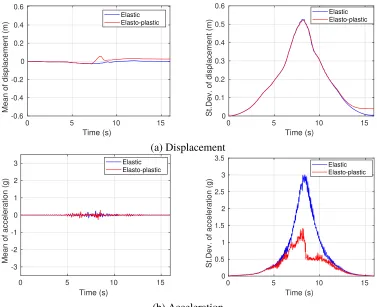
Figure 6 shows the simulated marginal mean and standard deviation of displacement, acceleration at the
ground surface. Note that a case with uncertain elastic material is also performed for comparison. Magnitude
of mean response is very small compared with those of standard deviation, and both the mean and standard
deviation of response is similar to the mean and standard deviation of input bedrock motion as shown in
Figure 4. It indicates the uncertainty of response mostly results from the uncertainty of seismic motion.
Due to material nonlinearity, permanent deformation is nontrivial with both the mean and standard deviation
of displacement are non-zero at the end of seismic loading. In addition, standard deviation of acceleration
decreases significantly due to probabilistic plastification of soil.
Figure 7 shows the stress evolution of soil at ground surface. The mean of stress is trivial compared to
standard deviation of stress. In addition, for uncertain elasto-plastic soil, standard deviation of stress drops
Division III
0 5 10 15
Time (s) -0.6
-0.4 -0.2 0 0.2 0.4 0.6
Mean of displacement (m)
0 5 10 15
Time (s) 0
0.1 0.2 0.3 0.4 0.5 0.6
St.Dev. of displacement (m)
(a) Displacement
0 5 10 15
Time (s) -0.2
-0.1 0 0.1 0.2
Mean of acceleration (g)
0 5 10 15
Time (s) 0
0.05 0.1 0.15 0.2
St.Dev. of acceleration (g)
(b) Acceleration
Figure 4: Marginal statistics of the seismic motion random process.
-1 15 -0.5
0
15
Coeff. of correlation
10 0.5
Time (s)
10
Time (s) 1
5 5
0 0
-1 15 -0.5
0
15
Coeff. of correlation
10 0.5
Time (s)
10
Time (s) 1
5 5
0 0
(a) Displacement (b) Acceleration
0 5 10 15 Time (s) -0.6 -0.4 -0.2 0 0.2 0.4 0.6
Mean of displacement (m)
Elastic Elasto-plastic
0 5 10 15
Time (s) 0 0.1 0.2 0.3 0.4 0.5 0.6
St.Dev. of displacement (m)
Elastic Elasto-plastic
(a) Displacement
0 5 10 15
Time (s) -3 -2 -1 0 1 2 3
Mean of acceleration (g)
Elastic Elasto-plastic
0 5 10 15
Time (s) 0 0.5 1 1.5 2 2.5 3 3.5
St.Dev. of acceleration (g)
Elastic Elasto-plastic
(b) Acceleration
Figure 6: Simulated surface response statistics of the soil deposit with uncertain elastic/elasto-plastic material and seismic motion.
0 5 10 15
Time (s) -30 -20 -10 0 10 20 30
Mean of stress (kPa)
Elastic Elasto-plastic
0 5 10 15
Time (s) 0 5 10 15 20 25 30
St.Dev. of stress (kPa)
Elastic Elasto-plastic
Division III
CONCLUSIONS
This paper presents a stochastic site response analysis with uncertain elasto-plastic soil and seismic motion.
The material parameters of soil deposit are assumed as non-Gaussian random fields while the uncertain
seismic motion is considered as a non-stationary bedrock motion. Hermite polynomial chaos is employed to
represent the soil random fields and seismic motion random process. The probabilistic constitutive model
of soil is von-Mises model with kinematic hardening and zero-elastic region. A stochastic finite element
analysis based on stochastic Galerkin method is performed to evaluate the ground surface response.
Uncertainties of simulated ground surface response mostly comes from uncertainties of input seismic
motion, and the mean response is trivial compared to standard deviation of response. Compared with the case
with elastic soil, permanent deformation is evident and standard deviation of acceleration drops significantly
due to probabilistic plastification of soil.
ACKNOWLEDGEMENT
Partial support from the US-DOE is appreciated.
REFERENCES
[1] Ghanem, R. G., and Spanos, P. D. Stochastic Finite Elements: A Spectral Approach. Springer-Verlag,
1991. (Reissued by Dover Publications, 2003).
[2] Hughes, T. J. R. The Finite Element Method: Linear Static and Dynamic Finite Element Analysis.
Dover Publications, Inc., Mineola, New York, 2000.
[3] Kramer, S. L. Geotechnical Earthquake Engineering. Prentice-Hall, Upper Saddle River, NJ, 1996.
[4] Lacasse, S., and Nadim, F. Uncertainties in characterizing soil properties. InUncertainty in Geologic
Environment: From Theory to Practice, Proceedings of Uncertainty ’96, July 31-August 3, 1996,
Madison, Wisconsin(1996), C. D. Shackelford and P. P. Nelson, Eds., vol. 1 ofGeotechnical Special
Publication No. 58, ASCE, New York, pp. 49–75.
[5] Metropolis, N., and Ulam, S. The Monte Carlo method.Journal of the American Statistical Association
44, 247 (1949), 335–341.
[6] Sakamoto, S., and Ghanem, R. Polynomial chaos decomposition for the simulation of non-Gaussian
nonstationary stochastic processes. Journal of Engineering Mechanics 128(2002), 190–201.
[7] Wang, F., and Sett, K. Time-domain stochastic finite element simulation of uncertain seismic wave
propagation through uncertain heterogeneous solids. Soil Dynamics and Earthquake Engineering 88