Transactions of the 17th International Conference on
Structural Mechanics in Reactor Technology (SMiRT 17)
Prague, Czech Republic, August 17 –22, 2003
Paper # D05-8
Process Data Reconciliation in Nuclear Power Plants
Magnus Langenstein, Josef Jansky BTB-Jansky GmbH, Leonberg, Germany
ABSTRACT
Process data reconciliation with VALI III is a method for monitoring and optimising industrial processes as well as for component diagnosis and condition-based maintenance in measurement technology.
Employing process data reconciliation in nuclear power plants enables thermal reactor power to be determined with an uncertainty of less than ± 0.5 %, without having to install additional precision instrumentation to measure the feed-water mass flow. This is equivalent to a measurement uncertainty recapture power uprate potential of about 1.5 %.
In addition, process data reconciliation permits any drift in the measured values to be detected at an early stage, yet still allows the reconciled variables (such as thermal reactor power) to be calculated with consistently high precision. Without reconciliation drifting of measured values for the feed water temperature or the feed-water mass flow could remain undetected, the thermal reactor power calculation may incorporate an unacceptably large deviation, negatively impacting both safety and economy.
KEY WORDS
: process data reconciliation, condition based maintenance, component diagnosis, VALI, datareconciliation, power uprate, acceptance test.
INTRODUCTION
All measurements are incorrect. The problem is, that with incorrect measurements the conservation laws cannot be fulfilled. The solution for this problem is the process data reconciliation with VALI III [1]. Process data reconciliation with VALI III is a mathematical-statistical method. When a plant model is created for an industrial process, all available or redundant measured variables must first be assigned to the model streams and units together with their respective measurement uncertainties.
The overdetermined system of equations that results when all available redundancies and secondary conditions (conservation laws) are taken into account is resolved with the aid of the Gaussian correction principle. Contradictory measured values are converted to unequivocal, "true" values for the measured variables, to obtain closed mass, energy and materials balances. The corrected covariance matrix is used to determine the corrected confidence intervals of the results. This method, described in VDI 2048 [2], is:
∗ The best possible quality control mechanism for identifying serious measurement errors, and
∗ A precondition of process monitoring, process optimisation and maintenance optimisation [3], [4], [5], [6].
Process data reconciliation is used in nuclear power plants, combined-cycle gas turbine power plants, coal-fired power plants, incineration plants, gas distribution systems and the chemical and petrochemical industries. This paper describes the theoretical basis of process data reconciliation with VALI III according to VDI 2048 as well as practical experience with online process data reconciliation in nuclear power plants (boiling water and pressurised water reactors).
THEORETICAL BASIS [2]
Gaussian correction principle
Corrections ν are made to the measured values
x
according to equation (1), in order to obtain estimated values (reconciled values)x
.ν x
x= + (1)
The corrections ν must be determined such that the quadratic form
min ν S ν
ξ -1
X
0 = ⋅ ⋅ ⇒ (2)
-1 X
becomes a minimum. The empirical covariance matrix SX is the estimated value for the uncertainty of the measured variables X. This general formulation also includes the existence of covariances, in other words the interdependencies of the measuring points. Equation (2) represents the general form of the Gaussian correction principle.
Quality control and detecting suspected tags (serious errors)
If the condition
1.96
≤
ii i
sν, ν
(3)
is not satisfied, the measuring point or the estimated value of the associated variance will incorporate a serious error. This measured or estimated value should consequently be challenged. In this condition the corrected measured value νi refers to the covariance matrix of the corrections.
Correlation coefficients for assessing delta measurements
The method described in VDI 2048 for assessing delta measurements takes account of the interdependency of values measured at different times but with the same chains. Correlation coefficients have to be defined between the values measured at different times, to allow random errors in these measuring chains to be considered. VALI III supports this.
Description of the method based on a simple example
The functional principle of process data reconciliation is described here with the aid of a simple example. Figure 1
shows a splitter. The entering stream is split into two partial streams. It is assumed that measured values which must satisfy the mass balance
3 stream 2
stream 1
stream m m
m• = • + • (4)
are available for the mass flows of all three streams (STREAM 1: 500 t/h, STREAM 2: 245 t/h and STREAM 3: 250 t/h). It can be seen that a simply overdetermined system exists, and that the mass balance cannot be closed with these values (refer to equation (5)).
h t 250 h t 245 h t
500 / ≠ / + / (5)
If, on the other hand, a standard deviation is assigned to each measured value (in this case ± 5 %, refer to Figure 1) and the correction calculation is performed, the "true" (reconciled) values are calculated taking account of the minimisation criterion in equation (2). In this example (without correlations), the minimisation criterion of equation (2) takes the following form:
minimum deviation
standard
value reconciled value
measured 2
=
−
=
∑
FUNCTION
OBJECTIVE (6)
The results report of the reconciliation run is shown in Table 1. They satisfy the mass balance equation (4); refer to equation (7)
h t 4 11 250.84 h
t 2 11 245.81 h
t 35 14
496.64± . / = ± . / + ± . / (7)
Table 1 result-report
OBJECTIVE FUNCTION = 0.103123 CHI-SQUARE = 3.84000 SUM OF SQUARE RESIDUES = 0.201948E-27
TAG NAME MEA.VAL. MEA.ACC. REC.VAL. REC.ACC. PENALTY P.U. ====================================================================================== STREAM1_M 500.00 5.00 % 496.64 2.89 % 0.10 t/h
STREAM2_M 245.00 5.00 % 245.81 4.56 % 0.10 t/h STREAM3_M 250.00 5.00 % 250.84 4.55 % 0.10 t/h
The hand calculation of this problem is documented in the following equations:
Measurement values with specified standard deviations
= ± = = ± = = ± = = h t 5 12 v where v 250 m h t 25 12 v where v 245 m h t 25 v where v 500 m m x3 x3 3 x2 x2 2 x1 x1 1 / , / , / intervall confidence 95 a implying 96 1 t with t v s 2 xi 2
xi = , %
= (8)
Covariance matrix Vector of measured values
=
2 1 2 1 2 1 1 1 1 2 1 xn xnk xni xn xkn xk xki xk xin xik xi xi n x k x i x x xs
s
s
s
s
s
s
s
s
s
s
s
s
s
s
s
S
(9) = 250 245 500 m m m 3 2 1 (10)Restrictions Vector of restrictions
0 m m
m1− 2− 3 = (11) f(x)=
(
m1−m2−m3)
=(0) (12)ν
x
f
x
f
x
f
∂
∂
+
=
(
)
)
(
where f(x) – Vector of contradictions, v - Corrective vector applied to the present example(
1 −1 −1)
= ∂ ∂ x
f and f x m m m 5
3 2 1− − = =
)
( (13)
and Sx The minimization problem
= 67 40 0 0 0 06 39 0 0 0 69 162 Sx , , ,
(14) ν⋅S−x1⋅ν−2λ⋅f
( )
x =ξ0 →Min (15)yields, after a few adjustments and the linearization of
ν
x
f
x
f
x
f
∂
∂
+
=
(
)
)
(
(16)the corrective vector
) (x f x f S x f S x f T x T
x ⋅
∂ ∂ ⋅ ∂ ∂ ⋅ ∂ ∂ − = −1 ν (17)
With the values specified above it can be calculated that
− − = ∂ ∂ ⋅ ∂ ∂ ⋅ ∂ ∂ − 168 0 161 0 673 0 , , , 1 T x T
x xf S xf
S x
f
(11) and
[ ]
− = − − − = 84 0 81 0 36 3 5 168 0 161 0 673 0 ν , , , , , , (18)
As a result, the restriction fulfilling values yield
= − + = + = = 84 250 81 245 64 496 84 0 81 0 36 3 250 245 500 ν m m m m m 3 2 1 , , , , , , (19)
The covariance matrix of corrections can be calculated as follows:
∂ ∂ ⋅ ∂ ∂ ⋅ ∂ ∂ ⋅ ∂ ∂ − = − x 1 T x T x
v f S f S f f S
S (20)
m1
m2
Implemented into the example it yields − − − − = 83 6 55 6 33 27 54 6 28 6 2 26 3 27 24 26 49 109 , , , , , , , , , v S (21)
and the corrected covariance matrix
= − − − − − = − = 83 6 55 6 33 27 54 6 28 6 2 26 3 27 24 26 49 109 67 40 0 0 0 06 39 0 0 0 69 162 S S
Sx x v
, , , , , , , , , , , , − − 84 33 55 6 3 27 54 6 78 32 2 26 3 27 24 26 2 53 , , , , , , , , , (22)
With the corrected covariance matrix and equation (1), the new corrected confidence intervals can be
calculated.vxi = sxi2 ⋅twitht=1,96implying a95%confidence interval (22) So you get the vector mNew without contradiction ± ± ± = h t 4 11 84 250 h t 2 11 81 245 h t 3 14 64 496 mNEW / , , / , , / , , (23)
The OBJECTIVE FUNCTION is calculated as 0.1 under the conditions specified for this example. There is no indication of any serious errors. The CHI SQUARE test, namely CHI SQUARE > OBJECTIVE FUNCTION, is passed (3.8 is greater than 0.1); refer to Figure 2. The calculated true values therefore do not need to be challenged.
It is thus clear that the VALI III system for process data reconciliation not only closes the mass balance but also provides an indication of serious errors. This is a very simple example. The data reconciliation will be improved, if more redundancies and a more complex model (more connections between the streams) exists.
Consideration of energy and materials balances
The IAPWS-IF 97 steam table, among others, is supplied with VALI III to permit thermodynamic system variables to be calculated for the water/steam process. VALI III also allows any chemical reaction equations (important, for example, when considering materials balances in combustion processes) to be mapped and integrated in the model. The functionality of VALI III is described in detail in the manual [1].
USE IN NUCLEAR POWER PLANTS
Process data reconciliation with VALI III [1] is used in nuclear power plants in order to:
∗ Perform acceptance tests, also for delta measurements (retrofitting, taking account of correlation coefficients)
∗ Evaluate maintenance activities like cleaning the compressor or condenser (delta measurements, taking account of correlation coefficients)
∗ Trace start-up activities in the plants
∗ Determine the mean coolant temperature more accurately
∗ Determine the thermal reactor power more accurately
∗ Use the reconciliation results as a calibration standard
∗ Reduce the cost of calibrating measuring points
∗ Evaluate exact performance indicators
Process data reconciliation in a 4-LOOP PWR (1350 MW)
306 306,5 307 307,5 308 308,5 309 309,5 310 310,5 311
7.9.98 7.9.98 7.9.98 7.9.98 7.9.98 7.9.98 7.9.98 7.9.98 7.9.98
Date/Time
Temperature in [°C]
JEC10CT711 Reconciled JEC20CT721 Reconciled JEC30CT731 Reconciled JEC40CT741 Reconciled JEC10CT711 Measurement JEC20CT721 Measurement JEC30CT731 Measurement JEC40CT741 Measurement
max. value
Fig. 1 Graph of the mean coolant temperature – 4 LOOP PWR
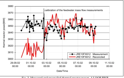
Fig. 2 compares the feed-water mass flow measurement of one steam generator with the reconciled values. The deviation between the measured feed-water mass flow and the reconciled mass flow is up to 13 kg/s, equivalent to 2 % of the total mass flow (accuracy range of the measuring devices). The direct influenceof the differences between the measured and reconciled feed-water mass flows is described in Fig. 3. The reconciled thermal reactor power is up to 30 MWth lower than the thermal reactor power based on measured data (main influence of the feed-water mass flow measurement). The aim is to use the reconciled values as a calibration standard and to calibrate the feed-water mass flow measurements such that the measured values correspond to the reconciled values. In this plant, in October 2002 the electrical output was increased with this method about 20 MWel see figure 2 and 3 and [7].
2100 2110 2120 2130 2140 2150 2160
29.9.02 0:00 1.10.02 0:00 3.10.02 0:00 5.10.02 0:00 7.10.02 0:00 9.10.02 0:00 11.10.02 0:00
Date/Time
sum of the feedwater massflow in [kg/s]
LAB60-90CF sum of all feedwater massflow measurements LAB60-90CF reconciled value
Fig. 3 Measured and reconciled thermal reactor power -4 LOOP PWR
Fig. 4 confirms how the feed water pressure measurement drifts upstream of one steam generator. The same graph also shows the PENALTY function over the drift period. The PENALTY function is the sum of all deviations of the model as a whole according to equation 6. During operation under 100 % load, the PENALTY value for this nuclear power plant is 70. The measuring point drift causes the PENALTY value to rise to 300. This rise in the PENALTY value is caused by the increasingly large deviation between the measured value and the reconciled value (refer to equation (6)). Changes to the PENALTY value therefore provide a quick and reliable indication of process changes or drifting measuring points without impairing the accuracy of the reconciled results.
56 57 58 59 60 61 62 63 64 65 66 67 68
23.7.00 00:00:00 02.8.00 00:00:00 12.8.00 00:00:00 22.8.00 00:00:00 01.9.00 00:00:00 11.9.00 00:00:00 21.9.00 00:00:00 Date/Time
Pressure in [bar]
0 50 100 150 200 250 300
PENALTY value
LAB60CP001 reconciled value LAB60CP001 measurement PENALTY Reconciled
Fig. 4 Drifting measuring point-4 LOOP PWR
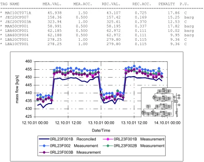
Measured values with a crucial influence on the magnitude of the PENALTY value are marked as suspected tags by the process data reconciliation system and stored in a separate file. Only those measured values which do not satisfy equation (2) are marked and stored. Table 2 shows a typical report. The report subsequently serves as a basis for the performance of condition-based maintenance on these measuring chains.
The VALI III model of this NPP has 96 redundancies; 219 measurements are implemented (temperatures: 95, mass flows: 42, pressures: 49, others: 33). Fig. 5 is a graph showing four measured values for a mass-flow measuring orifice
3800 3810 3820 3830 3840 3850 3860 3870 3880
29.09.02 00:00
01.10.02 00:00
03.10.02 00:00
05.10.02 00:00
07.10.02 00:00
09.10.02 00:00
11.10.02 00:00
Date/Time
thermal reactor power[MW]
as well as the associated reconciled value. Thereconciled value is approximately 7 kg/s less than the mean of the four measured values. If all three LOOPS are taken into account, the total measured feed-water mass flow is
approximately 19 kg/s higher than the reconciled mass flow (equivalent to a deviation of 1.4 % ifthe total measured feed-water mass flow is 1330 kg/s).
Table 2 Report of the suspected tags-4 LOOP PWR
TAG NAME MEA.VAL. MEA.ACC. REC.VAL. REC.ACC. PENALTY P.U. ====================================================================================== * MAC10CT071A 45.938 1.50 43.107 0.725 17.86 C * JEC20CP007 158.36 0.500 157.42 0.169 15.25 barg * JEC20CT003A 323.94 1.00 325.61 0.370 12.53 C * MAA50CP001 58.991 0.500 58.195 0.337 17.82 barg * LBA60CP001 62.185 0.500 62.972 0.111 10.02 barg * LBA60CP004 62.188 0.500 62.972 0.111 9.95 barg * LBA20CT001 278.25 1.00 279.80 0.115 9.36 C * LBA10CT001 278.25 1.00 279.80 0.115 9.36 C
425 430 435 440 445 450 455 460
12.10.01 00:00 12.10.01 12:00 13.10.01 00:00 13.10.01 12:00 14.10.01 00:00
Date/Time
mass flow [kg/s]
0RL23F001B Reconciled 0RL23F001B Measurement 0RL23F002 Measurement 0RL23F002B Measurement 0RL23F003B Measurement
Fig. 5 Feed water mass flow -3 LOOP PWR
Process data reconciliation in a 3-LOOP PWR (920 MW)
The influence of this deviation on the thermal reactor power is shown in Fig. 6. The reconciled thermal reactor power (approx. 2440 MWth) is around 30 MWth less than the thermal reactor power calculated on the basis of measured values (approx. 2470 MWth).
2400 2420 2440 2460 2480 2500 2520 2540
03.01.0 2 04:48
03.01.0 2 09:36
03.01.0 2 14:24
03.01.0 2 19:12
04.01.0 2 00:00
04.01.0 2 04:48
04.01.0 2 09:36
04.01.0 2 14:24
04.01.0 2 19:12
Date/Time
0YA00U510 Measurement 0YA00U510 Reconciled
± ? %
± 1,0 % reconciled uncertainty
Measurement uncertainty recapture power uprate
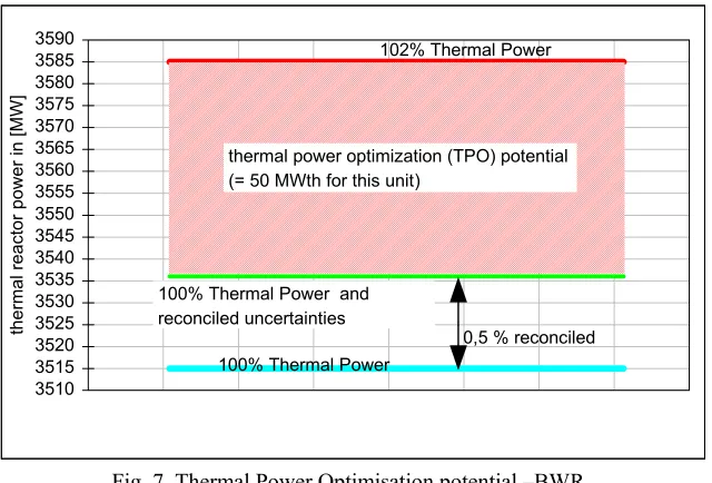
The thermal reactor power could be uprated by reducing the result uncertainties of the measured feedwater mass flow values, which are crucial for the thermal reactor power calculation. By reducing the result uncertainty to less than ± 0.5 % with the help of a process data reconciliation system, a measurement uncertainty recapture power uprate potential of 1.5 % could be utilised.
Fig. 7 shows a potential of 1.5 % (50 MWth) for a BWR plant in which process data reconciliation with VALI III has been installed for the past ten years. Compared to other methods of reducing the measurement uncertainty for thermal reactor power, such as installing more precise individual measuring instruments, the reconciled thermal reactor power principle combines consistently high accuracy with consideration of drifting measured values, for example of the feed water temperature or mass flow.
Fig. 7 Thermal Power Optimisation potential –BWR
Assessment of retrofit and maintenance activities
In order to permit assessments of delta measurements (before and after an activity) of the kind necessary in connection with retrofit or maintenance activities, process data reconciliation must also take account of correlation coefficients. The differences between the results with or without correlation coefficients are described taking the example of compressor cleaning work on a gas turbine. Fig. 8presents the results on a graph.
Fig. 8 Evaluation of a maintenance activity (Compressor cleaning in a CCGT) with and without correlation coefficients
3510 3515 3520 3525 3530 3535 3540 3545 3550 3555 3560 3565 3570 3575 3580 3585 3590
thermal reactor power in [MW] 0,5 % reconciled
100% Thermal Power
102% Thermal Power
thermal power optimization (TPO) potential (= 50 MWth for this unit)
100% Thermal Power and reconciled uncertainties
4,02 MW
1,16 MW
2,54 MW
3,92 MW
0 0,05 0,1 0,15 0,2 0,25 0,3 0,35 0,4 0,45 0,5
0 0,5 1 1,5 2 2,5 3 3,5 4 4,5 5 5,5 6 6,5 7 7,5 8 8,5
increase of electrical power output in [MWel]
Probability density
without correlation coefficients with correlation coefficients
increase of electrical power output with a probability of 95%
A power increase of 4.02 ± 1.77 MW is obtained if correlation coefficients are taken into consideration. If these correlation coefficients are neglected, the power increase is calculated to be only 3.92 ± 3.17 MW (result uncertainties corresponding to the 95 % confidence interval). If the power increase corresponding to 95 % probability is calculated, the figure is
∗ 2.54 MW with correlation coefficients, or
∗ 1.16 MW without correlation coefficients.
Compared to other methods (which do not take account of correlation coefficients), this method of assessing delta measurements with correlation coefficients therefore yields considerably more detailed information about the true power increase. As a result, the optimum time from a commercial point of view to repeat maintenance activities can be determined more accurately.
Furthermore, the method described here for assessing delta measurements enables:
∗ Power increases caused by RETROFIT activities to be determined more precisely, and
∗ A gradual deterioration of the plant as a whole, and hence of its efficiency, to be detected at an early stage on the basis of a reference condition (good condition of the plant).
CONCLUSIONS
The process data reconciliation method with VALI III describes industrial processes extremely accurately. The results can be used in nuclear power plants both for measurement uncertainty recapture power uprating and for condition-based maintenance. The potential financial benefits far exceed the necessary investment costs [8].
REFERENCES
[1]VALI III USER GUIDE, BELSIM S.A., Liege, Belgium, October 2001
[2]VDI 2048, “Uncertainties of measurement during acceptance tests on energyconversion and power plants -fundamentals”, October 2000
[3]U. Brockmeier; “Validierung von Prozeßdaten in Kraftwerken” VGB-Kraftwerkstechnik Issue 9/99 Pages 61-66 [4]E. Grauf, J. Jansky, M. Langenstein; Investigation of the real process data on basis of closed mass and energy
balances in nuclear power plants (NPP); SERA-Vol. 9, Safety Engineering and Risk Analysis - 1999, Pages 23-40; edited by J.L. Boccio; ASME 1999
[5]Grauf, E., Jansky, J., Langenstein, M.: Reconciliation of process data in nuclear power plants (NPPs), 8th International Conference on Nuclear Engineering (ICONE) April 2-8, 2000 Baltimore, MD USA
[6]M. Langenstein, J. Jansky: Process data validation in CCGT and nuclear power plants, Paper # O03/2, SmiRT 16, Washington DC, August 2001
[7]M. Langenstein: Betriebsdatenverwaltung und Analyse: Datenvalidierungssysteme, Einsatzbereiche, Effektivität und Potenzial; Fachtagung “Reaktorbetrieb und Kernüberwachung” der KTG-Fachgruppen “Betrieb und Reaktorphysik und Berechnungsmethoden”; 13. - 14. Februar 2003; Forschungszentrum Rossendorf