ABSTRACT
REEDY, JACOB DAVID. Proof of Concept for Novel Method of Quantifying Stability Margins for Non-Linear Phase-plane Controllers. (Under the direction of Dr. Andre P. Mazzoleni.)
This thesis proposes an original method for quantifying the stability of a phase-plane
controller called the Time Domain Analysis of Phase-Plane Stability, or TDAPPS. Phase-plane
controllers are a type of on-off, or ‘bang-bang,’ control system in which the vehicle’s reaction
control system is either active or inactive. It is difficult to come up with gain and phase margins
or otherwise determine the stability boundaries for a non-linear system. Current methods of
analysis are abstract, time-consuming, and yield a gain margin in the frequency domain. The
proposed TDAPPS method does not require in-depth knowledge of non-linear analysis tools and
provides gain and phase margins in the time domain. This thesis describes how a phase-plane
controller works, compares the proposed method to current practices, and tests its application to
the phase-plane control system for a space vehicle reminiscent of the Apollo capsule. The results
of this test are then confirmed via simulation testing to prove that the TDAPPS method is a
valuable analysis tool for non-linear control systems.
© Copyright 2018 by Jacob David Reedy
Proof of Concept for Novel Method of Quantifying Stability Margins for Non-Linear Phase-plane Controllers.
by
Jacob David Reedy
A thesis submitted to the Graduate Faculty of North Carolina State University
in partial fulfillment of the requirements for the Degree of
Master of Science
Aerospace Engineering
Raleigh, North Carolina
2018
APPROVED BY:
Dr. Andre P. Mazzoleni Dr. Larry M. Silverberg
Chair of Advisory Committee
DEDICATION
To my wife, Sarah, and parents, Marie and Dave, for constant love and support of all kinds.
BIOGRAPHY
Jacob D.P. Reedy was born in Reading, Pennsylvania and moved to Charlotte, North Carolina at
the age of ten. He attended North Carolina State University for his undergraduate education where
he received a Bachelor’s Degree in Aerospace Engineering. To pursue his goal of attaining a career
in the space industry, he immediately enrolled in the Master’s program at NC State. Under the
guidance of Dr. Andre Mazzoleni, he studied advanced dynamics, researched methods of active
trajectory control for high-altitude balloons, and developed a prototype Mars rover. Prior to
receiving his Master’s Degree, he accepted a job with Adaptive Aerospace Group, Inc. in
Hampton, VA. He is currently working there tackling projects such as simulating the entry,
descent, and landing phases of manned space capsules, performing controller stability analyses,
and conducting Monte Carlo analysis on small UAS. In his free time, he enjoys reading, playing
ACKNOWLEDGMENTS
I have many people to profusely thank for many different forms of support and encouragement. I
would like to start off by thanking thank my wife, Sarah, parents, Marie and Dave, and siblings
Sam, Olivia, and Ben for their constant love, strength, and support. I must also profusely thank Dr.
Mazzoleni for accepting me as a graduate student, mentoring me on several projects, and arming
me with knowledge and experience that has already served me very well in my young career. Next,
I owe a lot of gratitude to Keith Hoffler and Bruce Jackson of Adaptive Aerospace Group for
providing me with a fantastic opportunity to start my career and mentoring me over the last few
years. I would like to specifically thank Bruce Jackson for all the help in developing TDAPPS and
editing this document.
I also owe a thank you to many of my friends that helped me survive graduate school. First,
thank you to Chris Yoder for volunteering his time to help improve this thesis. I would like to
specifically thank Chris Yoder, Sachin Kelkar, Rajmohan Waghela, Jon Gatlin, Andrew Davis,
Michael Brueno, Keifer Ewing, and Zachary Tulbert for being great friends and supporters
TABLE OF CONTENTS
LIST OF TABLES... vi
LIST OF FIGURES... vii
1. Project Description ... 1
2. The Phase-plane Controller ... 3
2.1 Background ... 3
2.2 Description ... 4
3. TDAPPS Method ... 15
3.1 Description ... 15
3.2 Comparison with Describing Function Method ... 26
3.3 Simulink® Simulation Description... 28
4. TDAPPS Application ... 33
4.1 Apply to generic re-entry capsule ... 33
4.1.1 3-axis attitude control ... 35
4.1.2 RCS Jet cross-coupling ... 44
4.2 Discussion of TDAPPS results ... 54
5. Conclusions ... 64
6. References ... 66
APPENDIX...………... 68
LIST OF TABLES
Table 3.1 Equations for each of the firing curves in terms of controller parameters... 16
Table 3.2 Jet state flag value assignment based on the command from vehicle guidance... 21
Table 4.1 Nominal Apollo Command Module mass properties at entry interface... 34
Table 4.2 Initial Euler angle attitude and angular rates... 35
Table 4.3 RCS torque and corresponding angular acceleration magnitude in each axis... 36
Table 4.4 Initial Euler angle attitude and angular rates for the cross-coupling simulation... 44
Table 4.5 RCS jet thrust alignment unit vectors... 45
LIST OF FIGURES
Figure 2.1 Space Shuttle phase-plane space... 4
Figure 2.2 Phase-plane space plot for a simple phase-plane controller... 6
Figure 2.3 Top – Total Error vs. time; Bottom – Thrust versus time... 8
Figure 2.4 Phase-plane plot with hysteresis... 9
Figure 2.5 Top – Total Error vs. time; Bottom – Thrust versus time... 10
Figure 2.6 Single axis phase-plane controller with an applied external torque... 11
Figure 2.7 Phase-plane space with numbered intersection point to show a full analysis cycle... 12
Figure 2.8 Unstable phase-plane controller... 13
Figure 3.1 Example of phase-plane space with key terminology labels... 17
Figure 3.2 TDAPPS method flow chart... 19
Figure 3.3 Visualize aid for describing curve projection... 22
Figure 3.4 Classic control loop... 27
Figure 3.5 Top level of three_axis_phase_plane_exp.slx... 29
Figure 3.6 Plant model for the three-axis phase plane controller... 30
Figure 3.7 Top level of the phase plane controller subsystem... 30
Figure 3.8 Splitting phase plane controller between upper and lower bounds... 31
Figure 3.9 Phase plane controller upper level deadband logic model... 32
Figure 4.1 Depiction of CM body reference frame and general RCS jet locations... 35
Figure 4.2 Roll axis phase plane plot with no RCS cross-coupling... 37
Figure 4.3 Total error and torque time histories for the roll axis... 38
Figure 4.5 Pitch axis phase plane plot with no RCS cross-coupling... 41
Figure 4.6 TDAPPS results for the pitch axis... 42
Figure 4.7 Yaw axis phase plane plot with no RCS cross-coupling... 43
Figure 4.8 TDAPPS results for the yaw axis... 43
Figure 4.9 Roll-axis phase plane response of vehicle with cross-coupling... 46
Figure 4.10 Roll-axis total error and torque time histories... 47
Figure 4.11 TDAPPS analysis for roll-axis cross-coupling simulation... 48
Figure 4.12 Pitch-axis phase plane response of vehicle with cross-coupling... 49
Figure 4.13 Pitch-axis total error and torque time histories... 50
Figure 4.14 TDAPPS analysis for pitch-axis cross-coupling simulation... 51
Figure 4.15 Yaw-axis phase plane response of vehicle with cross-coupling... 52
Figure 4.16 Yaw-axis total error and torque time histories... 53
Figure 4.17 TDAPPS analysis for yaw-axis cross-coupling simulation... 54
Figure 4.18 Roll axis phase plane plot with 0.5 seconds of delay... 56
Figure 4.19 Roll axis total error and torque with 0.5 seconds of delay... 57
Figure 4.20 Yaw axis phase plane space from the doubled RCS torque simulation... 58
Figure 4.21 Yaw axis total error and torque plots from the doubled RCS torque simulation... 59
Figure 4.22 Yaw axis phase plane space from the quartered RCS torque simulation... 60
Figure 4.23 Yaw axis total error and torque plots from the quartered RCS torque simulation... 61
1. Project Description
A phase-plane controller is a type of ‘bang-bang controller’ often used to achieve
spacecraft attitude control [1,2,3]. It is a non-linear control system because the vehicle’s actuators
only have two states: on and off. For typical non-linear control systems, analysis is performed by
developing an error-dependent linear model of the controller and determining remaining stability
margin from the closed-loop gains at which the controller would become unstable. This method
has been used to analyze phase-plane controllers in the past but it requires several assumptions, is
abstract, time-consuming, and provides only a stability margin for gains in the frequency domain
[1,2,3]. While the result is certainly valid, it is not immediately intuitive as to how the gain margin
in the frequency domain will affect the actual dynamics of the vehicle. Nor does it provide insight
into the effect of time/phase delay on the system. It also requires an in-depth understanding of the
non-linear analysis method to successfully conduct in addition to interpreting the results.
This thesis project describes and examines an original method for determining the phase
and gain margins of a closed-loop system using a phase-plane controller in the time domain. The
time domain is more closely linked to the vehicle dynamics than the frequency domain, and it can
be simulated and visualized with relative ease. The proposed method is called the Time Domain
Analysis of Phase-Plane Stability (TDAPPS). The TDAPPS method is comprised of a programmed
algorithm that projects whether the system is stable or not at any given point along its trajectory,
and what the minimum time (phase) delay and/or change to the system gain would cause an
unstable response. Ultimately, the result is a time history of phase and gain margins along a
particular plant trajectory or maneuver. This makes it easier to identify problem areas where further
analysis may be required. The goal of this research is to show that the TDAPPS method can provide
freedom. Included will be studies of simulations across several different controller parameters and
target attitudes. This analysis would then aid engineers in designing and analyzing a system’s
phase-plane controller.
To accomplish this goal, this paper provides a brief, historical background on the use of
phase-plane controllers in general and on actual spacecraft and describe how a basic phase-plane
controller operates. Included in this will be a single axis example that delves into some of the
intricacies of this non-linear control method. Secondly, the paper will provide a detailed
description of the TDAPPS method including the theory and mathematics that it is based on. The
TDAPPS tool will also be compared to the non-linear stability analysis method that is most
commonly used, known as the Describing Function method (5,6). The next step will be to show
how the tool can be used to analyze an Apollo-like space capsule with 3-axis attitude control. The
first example analyzed investigates a simplified 3-axis model in which the thrusters are fired only
in the direction intended to correct the error in each axis. The second example removes this
assumption and applies reaction control torque cross-coupling. The analysis of these cases
provides an understanding of how the TDAPPS method can be used to analyze the stability of the
controller design and determine phase and gain margins for a system. It also illustrates the
flexibility of the TDAPPS tool, in that it can provide valuable feedback throughout a variety of
scenarios, with nominal effort on the part of the analyst. Finally, the results of the TDAPPS
2. The Phase-plane Controller 2.1 Background
“Bang-bang” control systems are commonly used across a wide variety of applications
from common household technology, such as thermostats, to satellites and other aerospace
vehicles. In dual-mode thermostats, for example, the user simply sets a temperature minimum
and/or maximum which act as the deadband values. If the temperature exceeds the upper deadband,
the air conditioning will turn on to lower it. If the temperature were to drop below the lower
deadband, the heat will activate until the room temperature is back within the given bounds. For
spacecraft, a special type of “bang-bang” controller, known as a phase-plane controller can be used
for precise attitude control during missions or phases that require quick and efficient attitude
changes or holds with minimal fuel consumption. It works much like the thermostat example,
except that there are two dependent variables, which are the vehicle attitude and attitude rate, as
opposed to just temperature.
Phase-plane control has been used on board many spacecraft for attitude control [1,2,3].
Despite the vacuum of space, there can still be gravitational, mechanical, and electromagnetic
disturbances that affect a vehicle’s attitude. Bang-bang control is very efficient for correcting these
small disturbances after they have built up too much error. Notably, the International Space Station
(ISS) and the Space Shuttle both employ(ed) phase-plane control for attitude maintenance during
on-orbit attitude correction maneuvers and when the two vehicles were docked together [1,2,3].
Figure 2.1 is a diagram of the phase-plane space as defined for the Space Shuttle. Although the
figure does not provide any values or explicit information, it is a great example of what the
‘phase-space’ looks like. Another attribute that makes the phase-plane controller so convenient is that this
a system. Vehicles that dock to the ISS are a good example of this where, for example, the Space
Shuttle docked to the ISS the coupling of the two vehicles creates an entirely different set of mass
properties and responses to effectors [1]. For traditional control system design, this would require
calculating a unique transfer function, but in this case the algorithm can simply switch to a different
set of gains, which may be more computationally efficient. The phase-plane controllers used for
these two vehicles are a great example of how flexible, efficient, and useful this type of control
design can be.
Figure 2.1 – Space Shuttle phase-plane space. [3]
2.2 Description
A phase-plane controller is a highly non-linear control method because it commands a
binary reaction control system (RCS), meaning that the control effectors are either on or off [4].
In other words, there are no linear “ramps” connecting the two states. In some spacecraft, the
control system actuators are small rocket engines, or jets, which cannot be throttled to provide
variable forces. Each jet has only two states: on and off. When a vehicle’s RCS jets are off, the
on the system, providing some control over the attitude. The job of the phase-plane controller is to
decide when the state of each jet needs to be changed to achieve or maintain the desired attitude
[4].
Determining the stability characteristics of such a non-linear system is not trivial. The
industry-accepted method used to perform such analysis is known as the describing function
method [5]. This method requires creating a linear estimator of the non-linear portion of the
controller and determining the gain margins from the combined linear and “quasi-linear” portions
of the plant [5,6]. However, upon studying the behavior of the phase-plane controller, a different
and unique approach was hypothesized. The proposed method determines phase and gain margins
in the time domain for each axis of a spacecraft and at every time step of a simulated trajectory.
This is accomplished by predicting the behavior of the phase-plane controller in phase-plane space
using the local inputs to the controller. This unique method is referred to as the time domain
analysis of a phase-plane controller (TDAPPS). The theory behind the TDAPPS analysis tool will
be discussed in detail starting with supporting information on the behavior of a simple, single axis
phase-plane controller.
A phase-plane controller is a relatively simple concept that can have added complexity
depending on the application. The simplest type of phase-plane controller requires accurate
knowledge of the current actual attitude and rate of the vehicle, which it compares to the
commanded attitude and rate to find two difference in each axis. All three axes of a vehicle can
have a separate phase-plane controller. For each individual axis, the attitude and attitude rate
differences are summed (a gain on rate error is included in some cases) to create a total error as
shown in equation 2.1.
This total error is compared to pre-determined error limits that are parameters within the
controller known as deadbands. If the total error does not exceed any of the deadband values, then
the error is in a ‘drift’ region and the RCS jets are commanded to be off. When any of the
deadbands are exceeded by the total error, an RCS jet is activated to correct the attitude and it will
remain on until the total error is back within the drift region [4]. When drawn in the phase-plane
space, these deadbands are represented by firing curves.
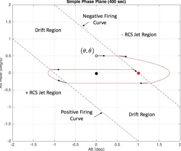
A convenient way to observe the behavior of the phase-plane controller is to plot the
attitude error versus the attitude rate error in what can be called phase-plane space [4]. Figure 2.2
shows the trajectory of the total error in phase-plane space with two firing curves that represent
the deadband parameters.
The hollow black circle marks the initial total error between the vehicle’s commanded and
actual attitude and rate, while the solid black circle marks the target of zero error. The solid red
dot is the location of the final data point. In this case, the initial point starts at the correct attitude
but has a rate that leads to a gradually increasing attitude error. The solid red line is the trajectory
of the total error and the black arrows show the direction that it is moving. The dashed lines are
the firing curves, which are generated from the deadband values. In this case, the deadbands are
set to a total error of ±1. Any time the total error crosses a firing curve, the RCS jet on-off state
changes as does the trajectory of the total error. The phase-plane controller successfully drives the
total error to within the tolerance even though the final point (red dot) does not match the target
(black dot). This is acceptable because the attitude rate has been driven to zero and the attitude
itself is within the deadbands, thus no further jet firings are required. It is also useful to show plots
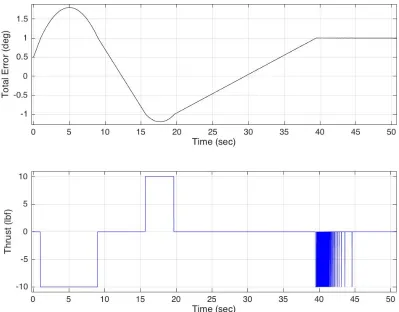
of the total error and RCS thrust versus time to illustrate the effectiveness of the controller. Figure
2.3 shows how the error is damped out within 40 seconds and how many jet firings it took to
achieve the damping. This system does require some simplifying assumptions including no
minimum on or off time for the RCS jets, which is unrealistic due to fuel tank pressure and
command frequency. Another assumption is that the controller has perfect knowledge of the
vehicles attitude and rates, as opposed to those derived from on-board sensors. Finally, the
examples of firing curves shown throughout this thesis are all linear. It is more common to find
firing curves are not infinitely linear, but that contain elbows (see Figure 2.1) or other
non-linearities [2,3,4]. The assumption that they are linear is valid in this case because the total errors
Figure 2.3. Top – Total Error vs. time; Bottom – Thrust versus time
It is notable in Figure 2.3 that between 38 and 40 seconds the negative jet is turned on and
off many times, which is not an efficient use of RCS fuel. This is typically improved by introducing
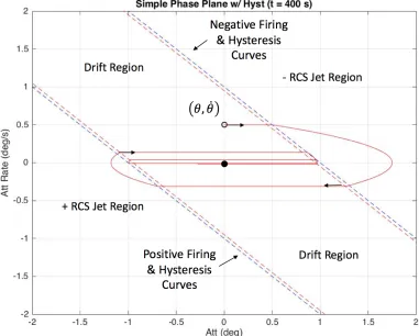
hysteresis to the system. Adding hysteresis complicates the logic required to implement the
phase-plane controller, but it can significantly increase the performance. Hysteresis is introduced as a
parameter to the system that shifts the firing curve in which the jet state would switch from on to
off [4]. Figure 2.4 shows a plot of the phase-plane space under the same conditions as Figure 2.2,
Figure 2.4. Phase-plane plot with hysteresis.
The hysteresis lines are the dashed red lines. They can be described as firing curves that
have been shifted slightly closer to the target. Their primary function is to delay switching the jet
state from on to off until after the total error crosses the hysteresis line. This prevents the rapid
firing of an RCS jet, also known as a high duty cycle, seen in the Figure 2.3 between 38 and 45
seconds. However, the addition of the hysteresis parameter increases the time it takes for the total
error to reach zero.
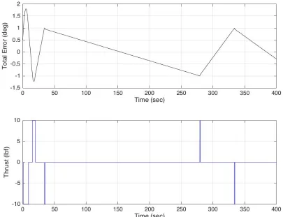
This type of controller behavior is ideal for a spacecraft in orbit that will be holding a
specific attitude for more than a few seconds because it burns very little fuel and holds the attitude
close to the commanded input [4]. It also helps that in orbit, the external forces on a spacecraft
over a period of minutes are often negligible. Figure 2.5 supports this claim by showing the total
adding hysteresis is clear when comparing Figure 2.5 to Figure 2.3. Figure 2.5 shows that only
five jet firings occur over the course of 400 seconds, whereas over 50 firings occur in 40 seconds
in the previous example.
Figure 2.5. Top – Total Error vs. time; Bottom – Thrust versus time
Both examples displayed in the previous figures are based on very simple single axis
systems with no external forces. In the case of a spacecraft in orbit there will be tiny external forces
from gravity gradients, solar pressure, payload operation, and cross-coupling forces from jet firings
in other axes that affect each individual axis even if the total error is in the drift region. Even these
small external forces will cause perturbations in the trajectory of the error [2]. Therefore, it is
pertinent to present an example with an applied external force so that the error trajectory can be
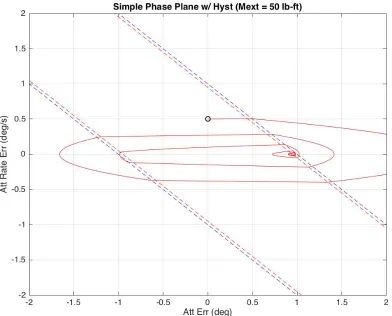
examined under conditions closer to what an actual orbiting vehicle would experience. Figure 2.6
torque of 50 lb-ft applied to the system. The external torque causes an angular acceleration on the
system that clearly affects the trajectory of the attitude and attitude rate. The error through the drift
region is no longer a horizontal line as seen in the previous figures, but is now parabolic. Even the
sections that are straight lines moving from one firing curve to the next can be described by a
parabola, which means that the motion can be predicted. This is the basis of the proposed TDAPPS
method.
Figure 2.6. Single axis phase-plane controller with an applied external torque.
Defining the stability of a phase-plane controller from the phase-plane space is
straightforward. Essentially, stability is evident if the attitude is closer to the desired target at the
end of some analysis cycle in the phase-plane space than it was at the end of the previous cycle.
An analysis cycle is defined a fixed number of times the RCS jet state has changed. For this study,
six times. To tell if the controller is stable over the span of one analysis cycle, the attitude rate
error at the initial jet state change can be compared to the attitude rate error at the final jet state
change. Figure 2.7 has numbers labeling each point where the state changes, which can also be
described as points of intersection with firing curves, and how a single analysis cycle is defined.
It is clear from this figure that the controller is stable at current conditions because the final
absolute attitude rate error at point (6) is smaller than the rate error at point (1). Note: The attitude
error is examined rather than the rate error, which cannot be used to determine stability in the same
way. As the rate error starts to decrease, the attitude error values at firing-curve intersection points
always approaches the deadband values. In other words, at low rates the attitude error values can
be greater than they were at the initial high rate condition, but still fall within the acceptable limits
even for a stable system.
The same idea can be applied to any of the phase-plane examples shown so far to show
that the results are stable. In fact, each of the phase-plane plots in the above figures can be shown
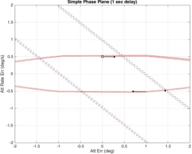
to be consistently stable by utilizing this method. Figure 2.8 shows an example of an unstable
phase-plane controller for reference. This instability was induced by subjecting the system shown
in Figure 2.4 to a one-second pure delay between a commanded RCS jet state change and the actual
jet’s response. The initial condition in Figure 2.8 is the hollow black circle, and the total error
trajectory is steadily moving away from the target (at point [0,0]) instead of towards it. The solid
black circle is the point at which a full analysis cycle is complete and, in this case, the rate error is
greater than where it is at the starting point. In other words, the magnitude of the attitude rate error
is increasing.
Observations gleaned from studying the behavior of a single-axis phase-plane controller
led to the proposal of finding instabilities in the time domain. The two observations that make the
TDAPPS method viable are that the trajectory of the total error in the phase-plane space is
parabolic for any steady non-zero external torque about the CG, and that the stability can be
determined based on an initial and final value of the attitude rate error. TDAPPS is a predictive
analysis tool that takes controller information at each time step and projects whether the response
in the system will be stable or not. After determining stability, it can also apply gain and time delay
margins to the system to determine the stability margins at each point. The information required
to perform this analysis includes the deadband and hysteresis parameters, the target attitude, the
current jet firing state, the current values of attitude and attitude rate error, and reasonably accurate
3. TDAPPS Method 3.1 Description
The TDAPPS method uses relatively simple algebra to predict the behavior of the
controller. The equations for a straight line and a parabola are the main mathematical components
of the algorithm. The difficulty lies in creating logic that determines which region the current error
is, the amplitude of any external moments acting on the vehicle, and which deadband the total
phase-plane trajectory will cross next.
The first step in developing the TDAPPS method is building a separate phase-plane space
for each of the controlled variables, which, for this research project, are the spacecraft attitude
Euler angles 𝜙, 𝜃, and 𝜓. The components of each phase-plane space are the firing curves,
hysteresis curves, and the resulting three firing regions created in each Cartesian space. The three
regions are referred to as the drift region, where no RCS jets are firing, and the positive and
negative firing regions. Constructing this space requires knowledge of the deadbands (𝐷𝐵12, 𝐷𝐵3$)
and hysteresis (𝐻𝑦𝑠𝑡) values for the controller being analyzed. For this study, it is assumed that
the positive and negative deadband and hysteresis values for each axis will remain constant
throughout each test case to make each of the firing and hysteresis curves linear. Because of this
they can be expressed using the slope intercept formula (Eqn. 3.1):
𝑦 = 𝑚𝑥 + 𝑏 Eqn. 3.1
In the phase-plane space the attitude error (𝜃'(() lies along the x-axis, while the attitude
rate error (𝜃'(() is along the y-axis. Attitude error is defined as the difference between the vehicles
current actual attitude and the commanded attitude. The attitude rate error is defined the same way.
𝜃'(( = 𝑚𝜃'(( + 𝑏 Eqn. 3.2
Knowing that the deadband and hysteresis parameters are constant with respect to each
axis of rotation (body roll, pitch, and yaw), and that the goal is to drive total attitude error to zero,
then enough information is available to determine the slope, 𝑚, and intercept, 𝑏. Using the upper
deadband as an example, the slope and intercept are expressed as follows:
𝑚 = − 𝐷𝐵12 , 𝑏 = 𝜃='>+ 𝐷𝐵12
where 𝜃='> is the target attitude angle for that axis. Combining the above equations with Eqn. 3.2
results in the equation for the negative firing curve:
𝜃'(( = − 𝐷𝐵12 ∗ 𝜃'((+ ( 𝐷𝐵12 − 𝜃='>) Eqn. 3.3
Eqn. 3.3 yields the negative firing curve even though the upper deadband was used to
formulate it because if the total error exceeds the upper deadband then the negative RCS jet needs
to be activated to correct the error. The equations for the remaining firing curve and the two
hysteresis curves can be generated using the same process, but with opposite signs. The equations
for each of these curves are central to the TDAPPS algorithm as they will be used to calculate the
projected points of intersection. Table 3.1 displays these four firing-curve equations in terms of
the deadband, hysteresis, and commanded attitude parameters.
Table 3.1. Equations for each of the firing curves in terms of controller parameters.
Negative Firing Curve 𝜃'(( = − 𝐷𝐵12 ∗ 𝜃'((+ ( 𝐷𝐵12 − 𝜃='>) Eqn. 3.3
Negative Hysteresis Curve 𝜃'(( = − 𝐷𝐵12 ∗ 𝜃'((+ ( 𝐷𝐵12 − 𝜃='> − 𝐻𝑦𝑠𝑡) Eqn. 3.4
Positive Firing Curve 𝜃'(( = − 𝐷𝐵3$ ∗ 𝜃'((− (𝜃='>+ 𝐷𝐵3$ ) Eqn. 3.5
Positive Hysteresis Curve 𝜃'(( = − 𝐷𝐵3$ ∗ 𝜃'((+ (𝐻𝑦𝑠𝑡 − 𝜃='>− 𝐷𝐵3$ ) Eqn. 3.6
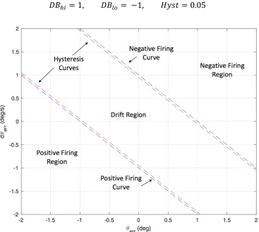
Figure 3.1 is a simple representation of the phase-plane space created using the above
equations. The hysteresis curves are represented by the dashed red lines and the firing curves by
the dashed blue lines. The negative firing region is the area in the upper right hand side of the
figure and is where the RCS jet firing to provide negative torque about the current axis is active.
The positive firing region is in the lower left area of the figure and is where the opposite jet will
be fired. The drift region, in the center of the figure, is the location at which no RCS jets are active.
Each of the firing curves are labeled along with the three regions that they divide the space into.
In this example, the controller parameters are set as follows:
𝐷𝐵12 = 1, 𝐷𝐵3$ = −1, 𝐻𝑦𝑠𝑡 = 0.05
Figure 3.1. Example of phase-plane space with key terminology labels.
Upon describing the phase-plane space for a vehicle, the basis of the TDAPPS algorithm
that the deadband and hysteresis values are not necessarily constant for any given vehicle, but
for proof of concept, they will be assumed constant throughout this study. Adding
non-linearities to the firing curves would complicate the logic required to run the TDAPPS
algorithm, but certainly does not make it impossible.
The logic involved in analyzing a controller’s stability will be specific to the complexity
of the phase-plane space as described above. However, the TDAPPS process that represents
the basics of the algorithm will not change. Figure 3.2 is a flow chart that defines the main
structure of this stability analysis method. Each step listed in the chart will be described in
detail as it pertains to the spacecraft being analyzed in this study, but again, the overall method
Figure 3.2. TDAPPS method flow chart.
The inputs to the algorithm at each time step include the attitude error vector (𝜃'((), attitude
rate error vector (𝜃'((), jet state flag vector, angular acceleration in the body frame (𝛼F), the
TDAPPS Method Flow Chart
Inputs: Att. Error, Rate Error, Jet State, Ang. Acc., Controller Parameters
1. Determine current region.
2. Determine trajectory shape.
3. Determine LAST firing curve crossed.
4. Determine NEXT firing curve crossed.
5. Project point of intersection. Return to 1. Terminate after a complete analysis cycle.
Inputs: Att. Error, Rate Error, Jet State, Ang. Acc., Controller Parameters
Drift Region Firing (+/-)
Region
External Torques?
Parabolic No
Yes
deadband parameter (𝐷𝐵12, 𝐷𝐵3$), hysteresis parameter (𝐻𝑦𝑠𝑡), and the commanded attitude
vector (𝜃GH=). The attitude error and attitude rate error vectors are defined by the difference
between the vehicles current actual state and its commanded state. Equations 3.7 and 3.8 describe
how they are calculated from simulation or measurement data to be provided to TDAPPS.
𝜃'(( = 𝜃IG#− 𝜃GH= Eqn. 3.7
𝜃'(( = 𝜃IG#− 𝜃GH= Eqn. 3.8
The deadband and hysteresis parameters are known quantities since they are parameters
defined in the design of the phase-plane controller itself. The commanded attitude vector is also a
function of the controller and is likely based on mission requirements. These quantities need to be
passed into the TDAPPS function so that the phase-plane space can be constructed and projections
can be made. The final input is the jet state flag vector, which is the value of the binary command
passed from the guidance to the RCS models that commands whether a specific jet is active or
inactive.
Upon receiving the appropriate inputs, the stability analysis algorithm begins with step one
from the flow chart (Figure 3.2), ‘Determine Current Region.’ This involves using logic to
decipher the value of the jet state flag. For the spacecraft that is studied in this paper, each rotational
degree of freedom has a positive and a negative RCS jet. Table 3.2 shows how values are assigned
to the jet state flag and what region that corresponds to in phase-plane space. If no jet is active, the
flag has a value of 0 and the total error is in the drift region. If the positive RCS jet is commanded
to be active, the jet has a value of 1 and the total error is in the positive firing region. Finally, if
the negative jet is commanded to be active the value is –1, and the total error is in the negative
Table 3.2 Jet state flag value assignment based on the command from vehicle guidance
COMMANDED ON BY GNC POSITIVE JET NO JET NEGATIVE JET
JET STATE FLAG VALUE 1 0 -1
PHASE SPACE REGION + Firing Region Drift Region - Firing Region
After determining the region in which the current total error resides, the algorithm can
move on to predicting the path that the error will take within that region. This corresponds to step
two in the flow chart, ‘Determine Shape Trajectory.’ This step is slightly more complicated as
there are multiple branches of logic to follow, but it is the same procedure for any given
application. There are two different possible paths that the total error will trace through the
phase-plane space: linear and parabolic. This is based on whether the vehicle is being subjected to any
external torques, thus providing an angular acceleration on the body during the (no RCS jets firing)
drift. If there are no external torques acting on the system (i.e. from aerodynamics, gravity gradient,
etc.) then the trajectory will be linear. This is only the case for an orbital spacecraft whose attitude
currently rests within the drift region of the phase-plane space. If the total error is in either of the
other regions or if the vehicle is subject to other external torques, then the trajectory in the
phase-plane space will be parabolic.
Steps three and four require the most complicated logic of the process. Now that the
algorithm has determined the shape of the trajectory, an equation for that curve can be realized. If
the trajectory is linear, the sign on 𝜃'(( can be used to determine which was the last firing curve
crossed and which is the next to be crossed. Referring to Figure 3.3, the current Cartesian position
of the total error is at the black circle showing that the rate error is greater than zero. Due to the
nature of the phase-plane plot, this means that the total error trajectory is going to cross the negative
the corresponding firing curves for a parabolic trajectory is slightly more difficult. Fortunately,
selection of the previous firing curve only needs to be completed on the first iteration of each cycle,
because data can be saved from one projection to the next.
Figure 3.3 – Visual aid for describing curve projection.
If the total error is in one of the firing regions, the selection of previous and next firing
curve encounter is obvious. A total error in the negative firing region (i.e. between points (2) and
(3) in Figure 3.3) means that the last firing curve crossed was the negative firing curve and the
next one to be crossed will be the negative hysteresis curve. The difficulty in this step crops up if
there is an external torque on the vehicle while in the drift region. Although this case will not be
specifically examined in this paper, a method for determining these conditions was developed and
Step five involves solving for the next point of intersection with a firing curve based on the
information gathered in the previous step. This is trivial in the case of a linear trajectory since the
rate error will be constant. The only thing that needs to be solved for is the attitude error, 𝜃'((,
which can be done by solving one of Eqns. 3.3 – 3.5 depending on which curve is currently of
interest. Once that next point of intersection is calculated, it is saved as the starting point for the
next iteration of the TDAPPS cycle. This step is also more difficult when a parabolic trajectory is
involved.
The only extra piece of information required to calculate the intersection of the error
trajectory with a firing curve is the angular acceleration that the RCS jet is supplying. This study
assumes that there are no external torques acting on the vehicle, which greatly simplifies the
calculation and projection of angular acceleration values during a TDAPPS analysis cycle. If this
assumption was not made, it would be very difficult to obtain the actual angular acceleration at a
given time step, which would also complicate projecting the vehicle’s trajectory through the
analysis cycle. However, thanks to this assumption, the angular acceleration (𝛼) values associated
with each section of the phase-plane space can be initialized in the algorithm using the RCS torque
(𝜏KLM) and vehicle inertia data ( 𝐼 ) as seen in Equation 3.9.
𝛼 = 𝜏KLM
𝐼 Eqn. 3.9
The next step is to develop the equation for the parabolic trajectory by observing a
relationship between the vehicle’s angular acceleration and the phase-plane space. Equation 3.10
shows this relationship and comes from taking the partial derivatives of the rate of change through
𝜕𝜃'(( 𝜕𝜃'(( =
𝜃'((
𝛼 Eqn. 3.10
By rearranging this equation and taking the partial derivative with respect to 𝜕𝜃'((, the attitude
error can be projected through the phase-plane space using the following:
𝜃'(( =𝜃'((
P
2𝛼 + Β
Eqn. 3.11
where B is a constant equal to the value of q when w is zero. This equation is valid for any parabolic
trajectory of the total error through the phase-plane space.
With these Eqns. 3.3 – 3.5, 3.10, and 3.11, a full cycle through the phase-plane space can
be projected. TDAPPS uses a logic tree to determine which of the four firing curves will be crossed
next and then, since the parabolic equation and the appropriate firing curve equation are in terms
of q, they can be solved simultaneously for 𝜃 using the quadratic formula. This provides two values
of 𝜃 at intersection points with the given firing curve and these examined in another logic tree to
determine the correct one. This process is repeated, projecting backwards in time, to find the value
of 𝜃 at the previous point of intersection with whichever firing curve has been most recently
crossed. With these two values of omega, the parabolic equation can be used to calculate the q
values at the intersection points and the trajectory throughout the current region has been projected.
This process is repeated a total of six times for each set of attitude and attitude rate errors to project
a cycle all the way around the phase-plane space. Finally, the initial attitude rate error and the final
attitude rate error values from the projection are compared and if magnitude of the final value is
less than the initial, the controller is declared stable for this point in time. A tolerance is applied to
account for minor increases in rate error that would be common when the total error is very small.
𝜃'((_T− 𝜃'((U ≤ 1𝑒XY Eqn. 3.12
If the conditions of Equation 3.12 are satisfied, the stability flag output is assigned a value
of 1 and considered stable. Otherwise, the flag is given a value of 0 and the system is considered
unstable. Also, if the rate error itself is less than 0.1°/s, the stability flag is automatically set to one
(stable). This helps to eliminate the condition in which the error is just barely greater than zero
such that when a jet is fired, it increases more than the tolerance.
After this algorithm is executed and the initial stability is determined, the same set of points
is passed through two more algorithms that do almost the same thing. Instead, the first algorithm
adds in an artificial time delay margin which simulates what would happen if the command was
not followed until sometime after it was given. The delay margin is initialized at 500 ms and the
stability of this new system is determined in the exact same way as before. Then the delay value
is updated using the Newton-Raphson optimization method to locate the point at which the
controller just barely becomes unstable. This value of additional time delay is the smallest amount
that can be added to the system to cause it to go unstable. This same method is applied to find the
positive and negative gain margins. If the open-loop system is initially stable, a negative gain
margin does not exist.
The outputs of the TDAPPS function are time histories of the stability flag, time delay
margin, and positive and negative gain margins. Each iteration of TDAPPS works from a
‘snapshot’ of the plant and control system, projecting ahead based on current parameters and
dynamics. This provides valuable insight at each point of the vehicles trajectory as to whether the
control system was stable or not and how much gain or phase delay would need to be induced to
launched to determine the causes of such a result and assess the effectiveness of the controller in
unique situations.
3.2 Comparison with Describing Function Method
A popular method used for analyzing the stability of non-linear controllers, including
phase-plane controllers, is known as the describing function method [5]. There are several
approaches to this problem including the absolute stability approach, which employs a
combination of Popov’s criterion and Siljak’s loop transformation, but requires fairly limiting
assumptions and has mainly been used to analyzed the roll channel of vehicle launch systems [6,7].
However, based on a recent literature review, the describing function method seems to be the most
widely used and accepted. Thus, it seems pertinent to briefly describe how a describing function
analysis is accomplished and compare the process and results to the TDAPPS method.
The describing function method is often billed as a frequency domain analysis for
non-linear control [5]. Therefore, the first step in this method is to fit the system dynamics into a classic
control loop as seen in Figure 3.4. This traditional loop consists of the controller, in this case
non-linear and the plant representing the dynamic response, which closes the loop on the system. The
reason for fitting the desired system into this loop is to use well-established methods to perform
frequency domain stability analysis on the system. The catch is, these methods require a linear
controller model, thus, a linear representation of the non-linear controller is required. Creating a
linear approximation of the phase-plane controller is the next step in the describing function
Figure 3.4 – Classic control loop [5].
Coming up with a reasonable linear approximation of a non-linear system is one of the
biggest challenges of this method because the analyst needs to create a linear transfer function in
the frequency domain that is specific to each non-linearity and is dependent on the amplitude of
the error signal. When there are more than one non-linear elements, this process needs to be
repeated for each. However, once the transfer function has been identified, several traditional and
well-known analysis techniques are available for use in determining margins [5]. Examples of
these include Bode and Nyquist plots which display the frequency response of the system and
allow for graphical determination of gains. The ability to evaluate the controller using classical
and modern controls techniques is a distinct advantage of the describing function method.
The TDAPPS and describing function methods use an entirely different process to estimate
stability margins and both have distinct advantages over the other. The TDAPPS method uses
straightforward math and logic to predict controller performance and then provides the margins
along with graphical feedback in the time domain. The describing function method requires
linearized approximations for any non-linear component of the controller, but then allows for
traditional analysis in the frequency domain [5]. This is a distinct advantage over the TDAPPS
method. The use of these established methods provides a lot more confidence in results and will
be the expectation of any control experts. However, the flexibility, ease of use, and unique
graphical methods that TDAPPS provides makes it an attractive option. It may also provide an
alternate means of checking gains calculated in another manner and describing these margins to
TDAPPS is also comparable to using brute force to determine margins. The brute force
method is applying gains to the controller in a simulation environment and changing them until
instabilities occur. This can be time consuming and could make it easy to miss conditions in which
the gains may be different. TDAPPS is a sort of faster, formalized brute force method. Using its
definition of stability, it calculates the margins for each axis and at each time step of a simulation.
This ensures that the minimum tolerable margins are defined for each simulation. The results can
then be confirmed by applying the specific gain to the simulation instead of estimating values and
running it multiple times.
Upon conclusion of the literature review and weighing the advantages and disadvantages
of TDAPPS and the existing techniques, it was determined that there was value in continuing to
develop TDAPPS as an alternate form of phase-plane controller analysis.
3.3 Simulink® Simulation Description
A MATLAB® Simulink® simulation was created to aid in the formulation and testing of
the Time Domain Analysis of Phase-plane Systems algorithm. Simulink® is a block diagram based
simulation tool that is often used to develop and analyze a wide range of systems and applications.
TDAPPS was developed using MATLAB® version R2015b, but has since been updated to
R2017b. The Simulink® model, three_axis_phase_plane_exp.slx, and its supporting suite of
MATLAB® scripts will be described in this section. Most of these files will also be included in
Appendix 6.3.
Figure 3.5 shows the top level of the simulation of a spacecraft attitude control example
plane controller. This has the traditional feedback loop in which the states are sent into the
controller to determine the changes needed to track the desired rotational states. The subsystem
labeled Phase-plane Cont. contains both the discrete phase-plane controller and a single reaction
control system. The inputs to the controller are the current attitude and attitude rate errors. The
outputs are the total commanded RCS torque and the variable called Jet_Flag, which denotes what
region of the phase-plane space the error in each axis currently resides. The commanded torque is
combined with any external torques (if desired) to create a total torque acting on the vehicle, which
is then sent into the Plant model. This continuous subsystem calculates the current angular
acceleration of the vehicle based on the total torques and the current body rates using the following
equation:
In Equation 3.13, 𝛼 is the angular acceleration, 𝜏 is the torque on the system, 𝜔 is the
angular rate, and [𝐼] is the vehicle’s inertia matrix. The angular acceleration is then integrated to
determine the attitude rate and attitude. These states are fed back into the controller for the next
time step. Figure 3.6 displays the Plant subsystem.
Figure 3.5 – Top level of three_axis_phase_plane_exp.slx. 𝛼^ 𝛼_ 𝛼` = 𝐼^^ 𝐼^_ 𝐼^` 𝐼^_ 𝐼__ 𝐼_` 𝐼^` 𝐼_` 𝐼`` Xa ∗ 𝜏^ 𝜏_ 𝜏` − 𝜔^ 𝜔_ 𝜔` × 𝐼^^ 𝐼^_ 𝐼^` 𝐼^_ 𝐼__ 𝐼_` 𝐼^` 𝐼_` 𝐼`` 𝜔^ 𝜔_
Figure 3.6 – Plant model for the three-axis phase-plane controller.
The more complicated part of this simulation model was the development of the
phase-plane controller itself. It was developed using Kubiak as a reference [4]. Figure 3.7 shows the first
level of the Phase-plane Cont. subsystem.
This level splits the input attitude error and attitude rate error into their respective axes and
feeds them into a separate phase-plane controller for each axis. The resulting commanded torques
are output as a vector into the plant model. The individual jet flags are combined into a vector and
saved as an output because they are essential for the TDAPPS algorithm. Digging down further
into the phase-plane controller itself, Figures 3.8 and 3.9 help describe the finer details involved.
Figure 3.8 is the level in which the controller inputs are split between the upper and lower deadband
logic models. In this simulation, the phase-plane space is symmetric about the zero-error location,
or the center of the Cartesian plot. This means that the deadband and hysteresis magnitudes are the
same for each firing curve, but the signs are opposite. The other inputs to each logic model are the
current total error in the desired axis and the values of RCS torque if the jet is on and off. The
outputs of both models are combined to form the commanded RCS torque and jet flag value for
the specified axis.
Figure 3.8 – Splitting phase-plane controller between upper and lower bounds.
The logic for both the upper and lower phase-plane boundaries are very similar, so just the
upper deadband logic is displayed in Figure 3.9. At this level, the total error is compared to the
jet is active and the jet flag value becomes negative one (or negative one in the lower bound logic)
to activate the negative RCS jet. This jet is referred to as the negative RCS jet because it reduces
the error from a positive value back down to zero. The hysteresis adds some complexity to this
logic because it only comes into play when the jet flag value is going from on to off. This is handled
by also checking the sign on the error value, which denotes what quadrant the error is in. If the
error is in the lower right quadrant, that means the hysteresis curve comes into play and it delays
the termination of the jet firing.
Figure 3.9 – Phase-plane controller upper level deadband logic model.
This simulation is initiated and run using a MATLAB script called run_3x_phaseplane.m.
This script creates a structure called SimIn, which is how all the initial conditions and parameters
are passed into the Simulink workspace. From this interface, the user can change these values of
these parameters for analysis purposes. After all the values of this structure are populated, the
simulation is executed for the user-specified amount of time. Finally, the outputs are saved to the
MATLAB workspace so that they can then be passed into the TDAPPS algorithm. The simulation
is run as a fixed-step model at 10 frames per second. This is the test bed that was utilized to conduct
4. TDAPPS Application
4.1 Apply to generic re-entry capsule
The time domain analysis of a phase-plane controller stability algorithm was originally
developed to aide in the evaluation of a capsule-like spacecraft’s control system. Space capsules
often require precise attitude adjustments or maintenance so that they can dock with other
spacecraft, point sensors at a target, or enter the atmosphere of some celestial body [2,3] at the
proper angle. For example, it is imperative that a capsule docking with the International Space
Station damp out any rates and hold a precise attitude so that the docking mechanisms will operate
correctly [1,2]. Since it is common to find a phase-plane controller in a capsule’s guidance,
navigation, and control system (GNC), the TDAPPS algorithm was tested using specifications for
an Apollo-like space capsule.
The simulation used to test TDAPPS is only concerned with the attitude of the capsule, so
the only information required are the mass properties and reaction control system design. Several
documents are online that contain the necessary information [8,9]. The nominal set of vehicle mass
properties in this simulation are defined using the Apollo 14 mission report when the vehicle is at
entry interface, or the point at which the capsule is about to enter the Earth’s atmosphere [10]. This
means that the Service Module (SM) is not included in this simulation. Table 4.1 shows the
Table 4.1 – Nominal Apollo Command Module mass properties at entry interface [8,9].
The only required information for the RCS model was the total magnitude of thrust that
the jets were capable of supplying. According to the Apollo Experience Report [10] the command
module RCS jets produced an average of 93 lbf of thrust. Unfortunately, data describing the
orientation and location of each jet on the CM could not be found. Instead, reasonable values were
assumed and the simulation was tested across a range of these values to try to incorporate the
different possibilities. Figure 4.1 is a drawing of the Apollo command and service modules. The
command module is on the left side of the image and is the resource used to estimate the locations
of the positive and negative RCS jets. The image also shows the orientation of the command
module body frame, which is important for defining the Euler angles and rotation rates of the CM.
This also helps with assigning the thrust alignment unit vectors to each RCS jet. Originally, the
jets were treated as if they were perfectly aligned with its respective axis; however, this
simplification was made only to test the simulation and TDAPPS method. Upon confirming that
the results were within the expected ranges, more realistic estimated unit vectors were applied such
Mass (lbs) 12715.1
Xcg (ft) 86.5
Ycg (ft) -0.0167
Zcg (ft) 0.475
Ixx (slug-ft^2) 5897
Iyy (slug-ft^2) 5281
Izz (slug-ft^2) 4763
Ixy (slug-ft^2) 44
Ixz (slug-ft^2) -373
Iyz (slug-ft^2) -25
that there would be cross-coupling of moments in other axes. Both the simple and cross-coupling
cases will be discussed in this section.
Figure 4.1 – Depiction of CM body reference frame and general RCS jet locations [9].
4.1.1 3-axis attitude control
Preliminary investigation of the usefulness of the TDAPPS algorithm was conducted with
the assumption that the RCS jets were perfectly aligned parallel to one axis. In other words, no
cross-coupling of RCS torques were generated. The initial attitude state error conditions of the
capsule can be seen in Table 4.2 and were defined in such a way that the controller would be forced
to damp out initial rates in each axis.
Table 4.2 – Initial Euler angle attitude and angular rates.
𝝓𝒆𝒓𝒓 (°) 𝜽𝒆𝒓𝒓 (°) 𝝍𝒆𝒓𝒓 (°) 𝝓𝒆𝒓𝒓 (°/𝐬) 𝜽𝒆𝒓𝒓 (°/𝐬) 𝝍𝒆𝒓𝒓 (°/𝐬)
These values were subsequently varied to provide a sweep through a range of slow rates to
a relatively high rate of rotation for a spacecraft. Also, due to differences in thruster location and
inertia values about each axis, the RCS torques and angular accelerations acting on the system are
different depending on the axis. Table 4.3 shows the torques and accelerations that each axis
experiences when its respective RCS jet is fired. There are a few assumptions regarding the RCS
model that were made to simplify the simulation. The first is that there are no minimum or
maximum on-off times for any of the RCS jets. This means that no matter when a command is
issued the system can respond, which is not always true of an actual physical system. Another
assumption is that the thrust is modeled as a perfect step-input to the system, which excludes the
typical dynamics and rise-time seen in actual engine performance.
Table 4.3 – RCS torque and corresponding angular acceleration magnitude in each axis.
Axis RCS Torque (lb-ft) Ang. Accel. (°/s)
Roll (x) ±325.5 ±0.0552
Pitch (y) ±558 ±0.1057
Yaw (z) ±558 ±0.1172
The simulation was run for 200 seconds with these initial conditions and the subsequent
simulation data was analyzed with the TDAPPS algorithm. The results are broken down by axis
and discussed in this section.
The vehicle began with a small 0.05°/s rotation rate about the roll-axis and Figures 4.2 and
4.3 show the time history of the capsules response to this condition. The black, hollow circle
represents the starting point of the total error and it is initially moving in the positive x-direction.
Since the vehicle is drifting slowly along the x-axis, the control system only needs to fire three
times to keep the error within the tolerable region. It should be noted that each time the jet fires,
secondary control law aiming to damp out this type of drift to avoid a limit cycle, but this feature
was excluded from the simulation. The reason for this is to confirm that the TDAPPS algorithm
provides valuable feedback when a short, burst jet firing occurs providing a rapid transition in the
region that the total error occupies.
Figure 4.2 – Roll axis phase-plane plot with no RCS cross-coupling.
-2 -1.5 -1 -0.5 0 0.5 1 1.5 2
Err (deg) -2
-1.5 -1 -0.5 0 0.5 1 1.5 2
dot
E
rr
(deg/s)
Figure 4.3 – Total error and torque time histories for the roll axis.
This data was fed into the TDAPPS algorithm and the resulting stability parameter
time histories can be seen in the plots of Figure 4.4. The first plot in Figure 4.4 is of the
roll-axis stability flag, which shows that the controller was considered stable (stability flag
value of one) throughout the entire simulation. As a reminder, the current definition of
stability (defined in section 3.1) is that the magnitude of the vehicle’s angular rate error is
less than or equal to the rate error at the previous jet-state change. Looking closely at the
phase-plane plot of the total error in Figure 4.2, the correction thrust is stronger than
necessary for the total error and the controller enters a low-frequency duty cycle. During
the period that TDAPPS shows that the vehicle is stable, but that this type of control method
may not be the most efficient for this regime of the attitude error. This analysis is backed
up by the gain margins that TDAPPS calculated for this axis.
0 20 40 60 80 100 120 140 160 180 200
Time (sec) -1.5 -1 -0.5 0 0.5 1 1.5
Total Roll Error (deg)
0 20 40 60 80 100 120 140 160 180 200
Time (sec) -400 -200 0 200 400
Figure 4.4 – TDAPPS results for the roll axis.
The second, third, and fourth plots in Figure 4.4 show the time delay and system gain
margins (positive and negative), respectively. The range of allowable delay values is between 0
and 0.75 seconds. This means that the roll axis can tolerate a maximum delay of 0.75 seconds
between the jet command and its response. However, that amount of delay is only tolerable briefly
at the beginning of the simulation. Otherwise, after the initial corrective firing at 20 seconds, the
system cannot tolerate much, if any, time delay in the roll axis. This make sense since the vehicle
is in a duty cycle where the total error is close to the target, so any abnormal conditions could
easily cause an increase in the rate error. This observation is further supported by the predicted
gain margins.
The positive gain margin has a range of 0 to 12 dB, or up to 4 times the nominal thrust
magnitude. A value of 0 dB means that no gain margin can be tolerated and this is the result for
when the controller initially enters the duty cycle. Note that the zero-gain margin condition is
0 20 40 60 80 100 120 140 160 180 200
Time (sec) 0
1 2
Stab. Flag
Roll axis TDAPPS results
0 20 40 60 80 100 120 140 160 180 200
Time (sec) 0
0.5 1
Delay (ms)
0 20 40 60 80 100 120 140 160 180 200
Time (sec) 0
10 20
Pos. gain (dB)
0 20 40 60 80 100 120 140 160 180 200
Time (sec) -20
-10 0
constant between the first and second jet command. This means that if an increase in effector
torque occurred, it would be enough to increase the magnitude of the total error instead of
decreasing it. This will be explored further when these results are tested in the simulation.
Similarly, the negative gain margin has a range of -12 to 0 dB. The margin of -12 dB correlates to
a 75% reduction of the nominal thrust. This value remains at 0 dB for most of the simulation,
except for the beginning and the times where the delay margin increases. The consistency of these
results, as well as the observations that can be made to support them, help to validate these initial
TDAPPS results.
The pitch and yaw axes were examined in a similar way and the results can be seen in
Figures 4.5 through 4.8. Note from Table 4.2, that the initial rate errors are different from the roll
channel. This provides two different examples on the usefulness of the TDAPPS method. For the
pitch axis, the error does not enter a limit cycle until after the second firing. The results for this
axis are reasonably straightforward. The results show that this axis is also stable throughout and
show consistent delay and gain margins. The gain margin set is again between -12 and 12 dB while
outside of the limit cycle, and each margin goes to zero when the total error is too small. The
amount of tolerable delay starts at 0.9 seconds, but it drops to 0 for the same periods that the gain
margins do. After entering the limit cycle, the same analysis from the roll axis can be applied; if
the total error is too small, it cannot afford any changes to the system. This does show that TDAPPS
is sensitive to these limit cycle and that either the stability condition needs to be changed, or a
change to the physical or control system needs to be made. In this case, the limit cycle is not
significantly inefficient since the rate error is low and the jets only briefly fire twice once it begins.
TDAPPS algorithm is that experimentation in changing parameters can be performed in a
simulation setting and then re-examined with relative simplicity.
Figure 4.5 – Pitch axis phase-plane plot with no RCS cross-coupling.
-2 -1.5 -1 -0.5 0 0.5 1 1.5 2
Err (deg) -2
-1.5 -1 -0.5 0 0.5 1 1.5 2
dot
E
rr
(deg/s)
![Figure 2.1 – Space Shuttle phase-plane space. [3]](https://thumb-us.123doks.com/thumbv2/123dok_us/1658768.1208077/14.612.134.484.271.471/figure-space-shuttle-phase-plane-space.webp)

![Table 4.1 – Nominal Apollo Command Module mass properties at entry interface [8,9].](https://thumb-us.123doks.com/thumbv2/123dok_us/1658768.1208077/44.612.229.382.128.307/table-nominal-apollo-command-module-properties-entry-interface.webp)