Second Order Approximations to GMM Statistics

(1)

ABSTRACT

KYRIAKOULIS, KONSTANTINOS. Second Order Approximations to GMM Statistics. (Under the direction of Alastair R. Hall.)

This dissertation uses second order approximations to study the finite sample behavior of statis-tics that are employed under the GMM setting.

We present a Nagar (1959) approximation to the MSE of the IV estimates, when the disturbances are elliptically distributed. The accuracy of the approximation is illustrated through a comparison of the Nagar-type expansion with the exact finite sample MSE, that was derived in Knight (1985). The comparison suggests that second order approximations can be quite accurate, even when the sample size is 60 observations. This, alongside with the fact that exact results are more difficult to derive and harder to interpret, suggests that second-order approximations are powerful alternatives to the standard, first-order, asymptotic approximations.

(2)

SECOND ORDER APPROXIMATIONS TO

GMM STATISTICS

by

Konstantinos Kyriakoulis

a dissertation submitted to the graduate faculty of

north carolina state university

in partial fulfillment of the

requirements for the degree of

doctor of philosophy

economics

raleigh

April 2006

approved by:

(3)

Biography

Konstantinos Kyriakoulis was born on September 25, 1975, to Nikolaos and Vasiliki Kyriakouli in Tripoli, Greece. He lived in Tripoli till the age of 14, when he moved with his family to Athens, Greece.

Konstantinos graduated from the 2nd_{Lyceum Ilioupolis}_{in June of 1993. He received a Bachelor} of Science in Economics from the University of Piraeus in 1997 and entered the Economics graduate program at Athens University of Economic and Business that same year. During his graduate studies, Konstantinos was fascinated by the gnostic field of econometrics and this led to a master thesis that was concentrated on the use of Artificial Neural Networks in finance. He received his Master of Science in Economics in 1999, and he entered the Economics’ PhD program at North Carolina State University in 2000.

He joined the SAS Institute Inc. in May 2005, and he is currently working in the development of SAS Credit Risk Management, a solution designed to perform regulatory and economic capital analysis.

(4)

ACKNOWLEDGEMENTS

I am grateful to my advisor and committee chair, Dr. Alastair Hall, for his enormous help through-out my studies. His guidance, support, time, and energy have been instrumental towards my success in this project; I wish that someday I will be able to help someone as much as he helped me! I would like to thank my committee members, Dr. David Dickey, Dr. Atsushi Inoue, and Dr. De-nis Pelletier for their good advice, insightful comments and valuable feedback. Their contribution towards the quality of this thesis is greatly appreciated.

I want to thank my parents Nikolaos and Vasiliki, and my sister Aggeliki, for all their love and support throughout my life. They were, they are, and they will always be, successful parents, sib-lings, and friends! Having them in my life made me realize that nothing is as important as family; if you can succeed to that, you can succeed in anything!

Last but not least, I would like to thank my wife Sofia, for her unconditional love and support throughout our life together. I would have never been able to achieve my dreams without her, and I would have never enjoyed my life the way I do. It is her smile that makes all my good days unfor-gettable, and is the same smile that makes the bad days unaccounted for; it is my single purpose in life to see her smile every single day!

(5)

List of Tables

4.1 The values ofµ2 _and_q/µ_for_T _{= 30 . . . .} ₆₂

4.2 The values ofµ2 _and_q/µ_for_T _{= 60 . . . .} ₆₂

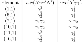
A.1 The non-zero elements ofvec(N γγ0_N0_{) and}_vec_(Λ0_γγ0_{Λ) for}_q_{= 2} _{. . . 116}

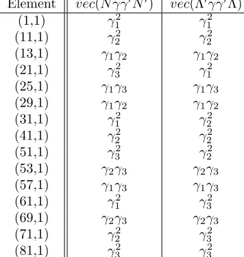
A.2 The non-zero elements ofvec(N γγ0_N0_{) and}_vec_(Λ0_γγ0_{Λ) for}_q_{= 3} _{. . . 117}

A.3 The non-zero elements ofvec(N γ⊥γ 0 ⊥N0) forq= 2 . . . 119

(8)

List of Figures

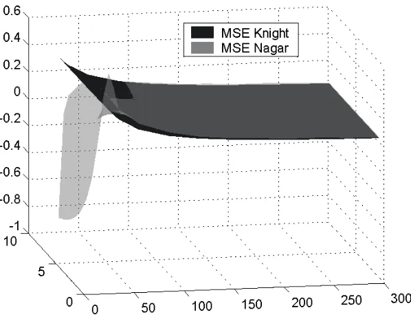
2.1 Nagar and Knight based BIAS of the IV estimates using elliptically distributed errors 26 2.2 Nagar and Knight based RMSE of the IV estimates using elliptically distributed errors 27

2.3 The second moment matrix to orderT−2: “Weak” instruments case . . . 28

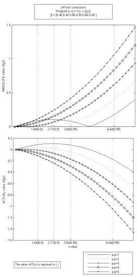
4.1 The correction term forT = 30 . . . 66

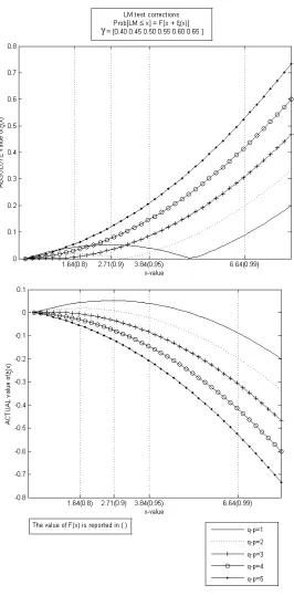
4.2 The correction term forT = 60 . . . 67

4.3 Comparison ofF(x) andF(x+ξ), forT = 30 and various values of q−p. . . 69

(9)

Chapter 1 Introduction

. . . “Edgeworth Expansions behave like the little girl with the curl in the famous

nursery rhyme: when they are good they are very, very good and when they are bad

they are horrid . . . [However, they] still provide a valuable source of information

about the adequacy of asymptotic theory. This is because they clearly signal those

regions of the parameter space where the corrections are small and those where

the corrections will be large. These, in turn, signal the regions where the crude

asymptotic does well and those where it does poorly.”

Phillips and Park (1988), p. 1066

The finite sample probability distributions of test statistics are available only for simple functions of the data where the likelihood function is completely specified. Unfortunately, the vast majority of the models used in practice do not satisfy this condition; in this case, econometric inference rests crucially on asymptotic analysis. The main mechanism of asymptotic analysis can be explained as follows: Suppose that the statistic of interest is denoted byS, and we wish to make inference using its sample analog, ˆST, which is based on a sample of sizeT. Then, asymptotic analysis rests on the assumption that T → ∞and uses theLaw of Large Numbers, Slutsky’s Theorem, and the Central Limit Theorem to derive the asymptotic distribution of ˆST; then, inference can be based on this asymptotic distribution.

(10)

Chapter 1. Introduction

enormously the econometrics field.

An important characteristic of large-sample analysis is that it is strictly valid only as the sample size goes to infinity; hence, it provides an approximation that may or may not be accurate in finite samples. It is, then, of interest to deduce the accuracy of these approximations. This can be done using either resampling techniques, or higher order expansions of the statistic of interest. The former methodology, for which bootstrap – see Efron (1979) – can be thought as the leading candidate, is based on resampling techniques and computer simulations that are calculating the empirical distribution of the statistic of interest. The latter methodology, for which Nagar (1959) and Edgeworth-type expansions are the leading candidates, is based on expanding the statistic of interest in a power series inT−1/2_{and then use its leading terms to get an improved approximation.} The question that arises naturally at this point is the following: Which method should be used? Resampling techniques or higher-order expansions? The answer to this question depends on the objective of the researcher. If we wish to increase the accuracy of a numerical calculation that is based on the data, for example a confidence interval or a rejection region, resampling techniques are preferred. If we wish to evaluate the accuracy of the large-sample distribution and deduce what drives the passage from the finite to the asymptotic results, higher-order expansions are preferred. The scope of our research falls into the second category. Thus, our analysis will be based on higher-order expansions.

We proceed with a description of the main developments in the areas of exact finite sample theory1_{, and second order approximations.}

1.1 Exact Finite Sample Analysis

One of the most influential papers on the finite sample properties of the OLS and 2SLS estimates was Bergstrom (1962). In his work, he did a comparative study on the finite sample properties of the OLS and 2SLS estimates of the Marginal Propensity to Consume (Keynsian setting). Bergstrom’s (1962) analysis was based on the assumption of normally distributed disturbances in the consumption function and a non-random investment series. Under these assumptions, he used a Monte Carlo study to analyze the performance of the estimates and his main result was that the 2SLS estimate is more accurate in finite samples.

Seven years later, Sawa (1969) generalized the analysis of Bergstrom (1962) into the case of a single equation with two endogenous variables. Using the assumption of normally distributed disturbances and non-random exogenous variables, Sawa derived the exact finite sample densities

1_{Even though we concentrate on second order approximations, it is important to see what are the developments}

(11)

of the OLS and 2SLS estimators. The results that he obtained agree with those of Bergstrom (1962), i.e. the 2SLS estimate is more accurate than the standard OLS. Specifically, using a set of simulation schemes2_{, Sawa (1969) showed that the bias of the OLS estimate is larger than the one} of the two-stage least squares in almost every setting studied.

The research up to this point had shown that, under the settings studied, the 2SLS estimates were clearly superior to OLS; as a result, researchers started focusing on the properties of the 2SLS estimates. Anderson and Sawa (1973) worked in the same setting as Sawa (1969) and they manage to show that the accuracy of the 2SLS estimates depends on the degree of overidentification. Specifically, as the degree of over-identification increases, the distribution of the 2SLS estimator becomes negatively skewed and exhibits more variation than what the asymptotic theory suggests.

Another important development in the area of the finite sample properties of the 2SLS estimates came from Phillips (1980). Recall that, in the area of the 2SLS estimates, the results that have been derived thus far were valid for models with a restricted number of endogenous variables. This restriction was overcome by Phillips (1980), who derived the exact finite sample density of the 2SLS estimates when the endogenous variables are n+ 1, where nis the number of the 2SLS estimates we wish to obtain. Phillips worked under the classical assumptions of normal disturbances and nonrandom exogenous variables and he managed to show that the finite sample moments of the 2SLS estimate exist up to the degree of overidentification. Additionally, he obtained the result that, as the degree of over-identification increases, the bias of the 2SLS estimates increases, while the dispersion decreases. This result was quite important by itself, although, as it was proven later by Buse (1992), is not necessarily true under more general settings3_{. An interesting by-product} of Phillip’s work was that, although finite sample densities can be calculated under more general settings, they are based on quite complicated formulae and thus, they are very difficult to interpret. The work of Phillips (1980) was complemented by Hillier, Kinal and Srivastava (1984) who derived the exact formulae for the moments of the instrumental variable estimation, using the same setup as Phillips (1980). However, the drawback of their work was very similar to the one of Phillips (1980); their formulae were very complicated and thus, difficult to interpret. Once again, it was evident that the exact finite sample analysis did not seem to provide as much insight as one would like. Note also that Knight (1985) derived similar formulae under the assumption of non-normality; however, his results shared the same drawback as their normal counterparts.

From the above analysis, two main points stand out: First, the usual asymptotic approximations are not always accurate, and second, the exact finite sample analysis is possible only under very restrictive scenarios (normality, and few endogenous variables). Additionally, the formulae of the

2

Sawa(1969) did simulations over different sample sizes, number of exogenous variables, and covariance of the endogenous variables.

(12)

finite sample expressions – for moments or densities – turns out to be quite complicated even under these, least complicated, settings. These findings increased the interest toward the derivation of higher order approximation – using the Edgeworth and Nagar type expansions. Such approximation have the potential of being less complicated, and they are still able to derive conclusions for the accuracy of the first order asymptotics. The development in this type of approximations is presented in the next section.

1.2 Second Order Approximations

Before presenting the development in second order approximations of moments and distributions, it will be helpful to give a brief description on the main algorithms used for these approximations.

1.2.1 The Methodology of Second Order Approximations

Higher order approximations can be easily described using the methodology introduced by Nagar (1959). Nagar showed that k-class estimators4 of simultaneous equations models can be expanded in a series where the successive terms are decreasing powers of T−1/2_{; the leading terms of this} expansion can be used to provide a higher order approximation to the moments of the k-class

estimators. This methodology has been utilized by many of the papers that we present later in this section. Additionally, it can also be used to approximate the higher moments of a statistic of interest and provide a higher approximation to its distribution. Concerning the approximation of distributions, an alternative algorithm, that is preferred when the calculation of the moments is complicated, is based on the expansion of the characteristic function of the statistic of interest; in this case, the higher order approximation can be found by a Fourier inversion of the expanded characteristic function. However, due to the complications that can arise in the Fourier inversion, this method has limited use. An algorithm that overcomes this complication was developed by Cavanagh (1983) and Rothenberg (1988). According to their methodology, the first step is to expand the statistic of interest as follows:

ST =S0+T−1/2S1+T−1S2+T−3/2S3+. . . (1.1)

whereS0has distribution functionFand densityf,Si,i= 1,2, are sequences of random variables with bounded moments asT goes to infinity, and their conditional moments are defined as

p(x)≡E(S1|S0=x), q(x)≡E(S2|S0=x), u(x)≡V ar(S1|S0=x)

(13)

Then, the Edgeworth approximation to the distribution ofS is

P r[ST ≤x]≈F

h

x− p(x)

T1/2 +

2p(x)p0₍_x₎₋₂_q₍_x_{) +}_u0₍_x_{) +}_c₍_x₎_u₍_x₎ 2T

i

(1.2)

where

p0(x)≡dp_dx(x), u0(x)≡ du_dx(x), c(x)≡dlog_dxf(x)

This algorithm simplifies greatly the procedure for obtaining an Edgeworth approximation since it does not require the Fourier inversion; the only part that complicates the analysis is the calculation of the expectations conditionally onS0=x. Usually, this is a rather minor complication in comparison with the inverse Fourier transform of the characteristic function; therefore, we have selected to use this algorithm for our analysis.

Having described the main algorithms used, we can proceed with an overview of the work that has been done on higher order approximations.

1.2.2 The Development of Second Order Approximations

As it was described before, the most influential papers in the area of higher order approximations is the one of Nagar (1959). Nagar (1959) worked under the assumption of normal, i.i.d. disturbances and he derived the second order approximation to the bias and MSE of the IV estimates. Despite that his results were not able to give a clear answer on how the bias and the MSE are affected by the instruments and their quality, they were very influential on the majority of the papers that follow.

Sargan (1975) derived a general theorem for the Edgeworth approximation to the distribution of thetratio of two-stage least squares andk-classestimators with non-stochastic exogenous variables. Under this setting, he managed to show that Edgeworth Expansions lead to valid higher order approximations5_{as long as the statistic of interest can be expressed as a function of variables that} possess moments of all orders6_{. Additionally, Sargan used these Edgeworth approximations in order} to improve the t-based confidence intervals. It turns out that the Edgeworth-based intervals are more accurate than the ones based on first order approximations.

Savin (1976) and Berndt and Savin (1977) analyzed the Wald (W), Lagrange Multiplier (LM) and Likelihood Ratio(LR) tests and they manage to show a systematic inequality among these three, asymptotically equivalent, tests. Savin (1976) analyzed the behavior of the three tests assuming a linear regression model where the disturbances follow a first order autoregressive process. For a

5

Generally speaking, a higher order approximation is valid if the remainder is bounded in probability and is of smaller order than the terms included in the expansion.

6_{Additionally, the statistic of interest must possess certain properties in a neighbor of the origin. These properties}

(14)

model with non-stochastic regressors7_{, they obtain the striking result that} _W _≥_LR_≥_LM_{, with} the equality holding only if the null hypothesis is exactly true in the sample. In other words, even though the three tests follow the same asymptotic distribution –χ2

rwhere ris the number of restrictions – their sample value might result to conflicting decisions8_{. Parallel to this work, Berndt} and Savin (1977) studied the behavior of the three tests in the case of a multivariate linear regression model and they concluded that the above inequality still holds. The next logical step was to derive higher order approximations for the distribution of these statistics; however, this had to wait for a few years before the necessarily theoretical foundation had been laid out. To that end, the work of Phillips (1977), Bhattacharya and Ghosh (1978), and Sargan (1980) was of extreme importance; these are analyzed below.

Phillips(1977) derived a theorem for the validity of the Edgeworth Expansions for sample sta-tistics with limiting normal distributions and random exogenous variables; in other words, Phillips extended Sargan’s (1975) paper to the case of random exogenous variables. In order to do this extension, Phillips used two sets of assumptions. The first concerns the properties of the error function that measures the error in the estimator or tests statistic; these were very similar with the ones of Sargan (1975) and dealt with the “smoothness” of the error function around the origin. The second set of assumptions concerns the properties of the underlying vector of variates,q; these were substantially different than Sargan’s since Phillips wanted to consider the case of random exogenous variables. Specifically, Phillips assumed that the joint density of √T q admits a valid Edgeworth expansion, the error of the expansion are suitably bounded9_{, and has bounded moments of all orders} as T → ∞. Even though these type of assumptions are hard to satisfy in the vector case, or for statistics more general than standardized means, Phillips theorem was a significant extension of Sargan’s (1975) and made the Edgeworth-type analysis available in more general settings.

During the same time, Bhattacharaya and Ghosh (1978) published one of the most important papers in the area of Edgeworth Expansions. In their work, they derived a theorem for the validity of the Edgeworth expansions that can be applied in a very wide class of statistics; their assumptions and result are presented below10_.

Specifically, suppose that X1, X2, . . . , Xn are d-dimensional i.i.d. vectors with mean µ and sample mean ¯X =n−1Pn

i=1

Xi. Additionally, letAbe the statistic of interest, satisfying thatA(µ) = 0. The function A that Bhattacharaya and Ghosh (1978) had in mind is of the form as A(x) = {g(x)−g(µ)}/h(µ), whereg and hare smooth functions11 _and _h₍_µ₎_>_{0. Then, assuming that}_(i)

7_{Savin(1976) also considered the case of a model with a lagged dependent variable. In this case, the LR tests}

possess the same critical region as in the non-stochastic case; the Wald tests does not. As a result, there is no any systematic relation between the tests.

8_{Because of the inequality, no conflict arises when the Wald test fails to reject}_H

0or when theLMtest rejectsH0. 9_{The bound must satisfy certain properties; see Assumption 2, Phillips (1977).}

(15)

the functionA hasj+ 2 continuous derivatives in a neighbor ofµ, (ii) E(||X||j+2₎_<_∞_and _(iii) the characteristic function,xofX satisfies lim sup

|t|→∞ |

x(t)|<1, thec.d.f. of the standardized statistic can be expanded as

Pn1/2A( ¯X)/σ≤x= Φ(x) +n−1/2p1(x)φ(x) +n−1p2(x)φ(x) +. . .+n−j/2pj(x)φ(x) +o(n−j/2) (1.3) wherepj are polynomials of degree at most 3j−1, with coefficients depending on moments ofX up to orderj+ 2. In other words, the standardized statistic admits a valid Edgeworth expansion.

The above result can be applied to all statistics that are expressed as smooth functions of sample moments; it is due to this characteristic that the paper of Bhattacharaya and Ghosh (1978) is considered a pioneering work in the area of Edgeworth expansions. Additionally, their methodology open the way for the analysis of even more complex settings; the description of these settings follows immediately.

Sargan (1980), building upon his 1975 work and using very similar conditions, he derived a theorem for the validity of the Edgeworth expansions in the case of χ2 distributed criteria. His results were derived assuming a simultaneous equation model with non-stochastic exogenous vari-ables and normally distributed disturbances. Additionally, Sargan (1980) demonstrated his result by considering the case of testing for misspecification in a single equation estimated by instrumental variables. Sargan’s (1980) work was the first12 _{one that dealt with}_χ2 _{distributed statistics and, to} quote Sargan himself13_:

[ Sargan(1980, p. 1137] . . . It seems likely that an extension of the theorem in this paper could be made using an approach through characteristic functions, as in Sargan (1976), or as in Phillips (1975) paper. This type of approximation can then be expected to give a basis for choice between the many asymptotically equivalent test criteria which arise in econometrics.

Two years later, Evans and Savin (1982) revisited the conflict between W, LM, and LR tests in the context of the linear regression model. Evans and Savin (1982) showed that if one uses some correction factors for theχ2 _{critical values then, the probability of conflict between the three} statistics is negligible. These correction factors were derived from an Edgeworth approximation to the distribution of the test statistics. Hence, their worked showed that the Edgeworth approximation toχ2_{distributed statistics is capable of providing important refinements.}

zero

12_{Rothenberg had dealt with Edgeworth Expansions of multivariate test statistics in a 1977 discussion paper.}

However, to our knowledge, Sargan’s work was the first published paper that dealt with higher order approximation ofχ2 _statistics.

13_{In the following quote, Sargan is referring in a 1975 discussion paper of Phillips. This discussion paper was}

(16)

The next important development in the area of Edgeworth Expansions came by Sargan and Satchell (1986). In their work, they derived a theorem for the validity of the Edgeworth expansion to the distribution of estimators of autoregressive equations with normal, white-noise disturbances. Sargan and Satchell (1986) also showed that their assumptions were satisfied in the case of a linear dynamic equation with normal errors. This work broadened the availability of Edgeworth expansions and showed that they can be used not only in static, but in dynamic models as well.

Another paper at the end of the ’80s, that utilized Edgeworth expansions in order to shed light on the finite sample performance of statistics, was the one by Phillips and Park (1988). The scope of their work was to use Edgeworth expansions to explain why the Wald test is not invariant to (equivalent) transformations of the null hypothesis. In their work, they first derived an Edgeworth expansion of the Wald statistic, and then used its higher order terms as a way of explaining why different formulations of the Wald test perform better than alternative forms (in finite samples). Their analysis indicated that these higher orders“provided enough additional information to capture the main distributional effects that are incurred by using alternative forms of the Wald test”. Their paper didn’t provide guidance on which is the best way to form a test. However, using their approach, one can identify how adequate the asymptotic theory is likely to be for different formulations of the restrictions. Additionally, in simple settings, the correction terms were able to suggest how to transform the restrictions so that the asymptotic approximation is improved.

An extension to the case of autocorrelated disturbances came from Rothenberg (1988). In his work, Rothenberg considered the case of a linear regression model where the error covariance matrix is based on an unknown parameter vector; in this setting, testing a hypothesis about the slope coefficient requires a robust estimator of the covariance matrix. Rothenberg derived an Edgeworth expansion for this type of statistics and he concluded that, under these settings, the second order correction terms can be quite large, even in very simple models (e.g. anAR(1) model with normal disturbances). Hence, his result came to reinforce the notion that first order asymptotic theory might not behave as well as expected. We note that, in this paper, Rothenberg derived the Edgeworth expansions using an algorithm developed by Cavanagh (1983); we underline that this algorithm we presented earlier, and we will be using it in our analysis.

(17)

explanatory power of those already included14_.

The only “missing” part in Buse’s (1992) formulae is that it wasn’t informative for the trade-off, if any, between bias and mean squared error. In order to answer this question, Hall and Peixe (2003) used the formulae of the mean squared error (MSE), as it was derived by Nagar (1959), in order to numerically evaluate the effect that the inclusion of instruments have on the MSE. Similarly to Buse’s (1992) analysis, they wanted to identify how the quality of instruments affects the bias and the MSE. To do that, they used the linear IV model to estimate a single parameter using a set of nine instruments. From this set, four instruments were considered “good” and five were considered “bad”15_{. Then, they computed the IV estimator using five different instruments sets,} each one consisting of four instruments; the only difference between these sets is the number of good or bad instrument included. In their computations, Hall and Peixe (2003) manage to show that the inclusion of a “bad” instrument will increase both the bias and the MSE. If a good instrument is included, the MSE is always decreased; the effect on the bias however is not that clear. Specifically, the inclusion of a good instrument might increase or decrease the bias, depending on the number of good instruments already included. Based on this result, one can conclude that:

“There is a far more complex relationship between the behaviour of the estimator and

the properties of the instrument vector in finite sample than is predicted by asymptotic

theory.” Hall (2005), p. 215

One of the most recent developments in the area of second order approximations is due to Newey and Smith (2004). In this paper, Newey and Smith (2004) studied a second order asymptotic approximation to the bias of GMM and Generalized Empirical Likelihood (GEL) estimators16_{, in} nonlinear static models with independent and identically distributed data vector. They manage to show that the bias of the GMM estimates is the sum of:(i)the bias of the optimal17_{GMM estimator} (BI),(ii) the bias due to the estimation of the variance of the moments (BS),(iii)the bias due to the estimation of the mean of the first derivative of the moments (BG), and (iv) the bias due to the first step estimation (BW). Similarly, the bias of the Continuous Updated GMM estimator is the sum ofBI,BG, andBS. Two very important results stand out in this work: First, it turns out that overidentification introduces bias from many sources since, when it is absent, all the terms but

BI are equal to zero. Second, the CU-GMM has smaller finite sample bias than GMM. Note that the smaller bias of the CU-GMM estimates was partially known from earlier work, such as Imbens

14_{The work of Buse (1992) showed that the result of Phillips (1980) is not true in general.}

15_{The notion of “bad” instruments does not mean that they are redundant. It rather means that they are nearly}

redundant given the good ones. For more details, see Hall and Peixe (2003), or Hall (2005)

16

The GEL estimators includes the Empirical Likelihood (EL) (Qin and Lawless, 1994), Exponential Tilting (ET) (Kitamura and Stutzer, 1997) and Continuous Updating (CUE) (Hansen, Heaton and Yaron, 1996) estimators.

17_{The optimal GMM estimator is the one based on the true variance and first derivatives of the moments; it is}

(18)

(1997)18_{, and Imbens (2002)}19_{; however, Newey and Smith’s (2004) work was the first one to provide} a theoretical comparison of the two estimates.

Just a year later, Anatolyev (2005) extended the Newey and Smith (2004) work to the case of stationary time series with serial correlation. Specifically, Anatolyev (2005) considered GMM esti-mators that use Heteroscedasticity and Autocorrelation Covariance (HAC) matrices, and smoothed Generalized Empirical Likelihood (GEL) estimators. His main results parallel the ones of Newey and Smith (2004). Specifically, the smoothed GEL removes the bias component that is associated with the correlation between the moment function and its derivative (BG, in the notation presented above). Additionally, the results of Anatolyev (2005) also depend on the third moment (which, due to the serial correlation, includes both contemporaneous and across time moments) of the moments function that, even in the case of GEL, can be removed only by a careful choice of the kernel. Over-all, the work of Anatolyev (2005) suggested that the bias of GEL estimates is smaller than the one of GMM20_.

During the very recent years, research interest has focused on the case of weak instruments and higher order approximations. At this point, we underline that the testing of inefficiencies in the case of weak instruments were analyzed earlier21; however, the second order approximations of test statistics in the case of weak instruments were analyzed only recently. Moreira, Porter, and Suarez (2005) showed that, if instruments are weak, the Wald and Likelihood Ratio statistics may not admit a valid Edgeworth Expansion. Specifically, if the instruments are weak, the statistics do not satisfy the “smooth function” assumption of Bhattacharaya and Ghosh – the derivatives of the functions evaluated atµare equal to zero. Hence, in the words of Moreira, Porter and Suarez (2005)“it is not obvious whether these statistics actually admit second-order expansions, and, if they exist, how to

prove their existence”. Thus, in this setting, the researchers are better off using alternative statistical procedures that will not break down; such procedures are(i)the K statistic – see Kleibergen (2005) – that uses a Jacobian estimator22 _{that is asymptotically uncorrelated with the sample average of} the moments, or(ii)a combination of the K statistic and the conditional likelihood ratio test, that was introduced by Moreira (2003).

At this point, it is important to underline that the work of Newey and Smith (2004) and Anatolyev (2005) provide only a partial assessment since they do not explore the nature of the bias-MSE trade off. This trade-off is studied in the work of Peixe, Hall, and Kyriakoulis (2006). In their work, they

18_{Imbens (1997) studied a nonlinear covariance structure model and he found the EL has smaller bias than GMM.} 19_{Imbens (2002) studied the properties of ET when applied to dynamic panel data with fixed effects, and finds that}

ET has smaller bias than GMM.

20

However, this work didn’t consider the bias/MSE trade off.

21_{Dufour (1997) showed that the Wald-type confidence intervals do not have correct the coverage probability; Wang}

and Zivot (1998) showed that the likelihood ratio test does not have correct size.

(19)

derived the Mean Squared Error of the IV estimates when the errors are elliptically distributed23_. Their work is based on Nagar (1959) type expansions, and generalizes the work of Buse (1992), which dealt with the second order bias of the IV estimates under non-normality. To assess the accuracy of this approximation, they compare their formulae with the exact finite sample results of Knight (1985)24_{. This comparison suggests that the accuracy of the Nagar type approximation depends} on the quality of the identification. The approximation error is largest in designs characterized by weak identification. However, in designs where identification is not weak, the approximation can be very accurate even in relatively small samples. This comparison has a twofold effect: First, it provides a measure for the usefulness and the accuracy of Nagar-type approximations. Second it identifies the settings, under which, the insights gained from the results of Buse (1992) and Newey and Smith (2004) can be taken to be accurate. We note that neither Buse (1992), Newey and Smith (2004) nor Anatolyev (2005) provide numerical evaluations of the accuracy of the approximations. Additionally, Peixe, Hall, and Kyriakoulis (2006) used their formulae to consider the impact of additional instruments on both bias and mean squared error. The main conclusion drawn from this analysis is that the introduction of poor quality instruments tends to increase both bias and MSE; the introduction of good instruments reduces the MSE but can either increase or decrease the bias according to the setting25_{. Second, we use the results to examine the performance of Andrewss} (1999) method for instrument selection. Finally, they used their MSE formulae to evaluate the Andrews (1999) moment selection criteria. Their result suggests that Andrews (1999) MSC does not tend to select the choice of instruments which minimizes either bias or MSE. Overall, these results suggest the use of a moment selection criterion which can distinguish good instruments from bad instruments; such a criterion has been proposed by Hall and Peixe (2003).

The above analysis has concluded the presentation of the current literature. The rest of our work is structured as follows.

Chapter 2 uses the IV model under non-normality and compare its second order bias and MSE with its exact, finite sample, values. The second order approximation to the bias is due to Buse (1992), while the one of the MSE is based on the work of Peixe, Hall, and Kyriakoulis (2006); the finite sample analysis is due to the work of Knight (1985). This comparison illustrates the accuracy of the second order approximations to the moments of the IV estimator and serves as a necessary stepping-stone for the rest of our analysis. Specifically, according to Rothenberg (1984)approximate moments play a key role in developing approximate distribution functions. Thus, one cannot expect that the Edgeworth expansion will be accurate if the moments of the IV estimate, which can be

23_{This class of symmetric distributions includes members with different degrees of fatness of tails, as the}

multi-normal, the multivariate t distribution and some mixtures of normal distributions.

24

This analysis is presented in Chapter 2 of this work.

(20)

considered as the most commonly used GMM estimate, are not approximated accurately; that is why we refer the next chapter as a “necessary stepping tone for the rest of our analysis”.

The Edgeworth Expansion of the LM test, as it is employed in the GMM case, is presented in Chapter 3. The analysis is based on two central assumptions, which are quite common in the higher order approximation literature: first, the data are independent and identically distributed, and second, the parameter vector is fully restricted under the null. Note that, due to second assumption, the LM test is a natural candidate since its calculation utilizes only the restricted estimates.

Chapter 4 presents a Monte Carlo simulation. The simulation uses the IV model to identify what drives the difference between the Edgeworth and the first order asymptotic approximation to the distribution of the LM test.

(21)

Chapter 2 Evaluating the accuracy of second order

approximations

In this chapter we evaluate the accuracy of the second order approximation of moments. This comparison is performed in a linear IV setting, under the assumption that the disturbances follow a potentially non-normal distribution. The accuracy of the second order approximations is evaluated numerically, by comparing the second order bias and MSE of the IV estimates with their exact, finite sample, counterparts; this comparison is done for different sample sizes and degrees of “non-normality”1_.

We begin by presenting the setup used, and the theorems that our analysis will be based on.

2.1 Model and assumptions

Our analysis considers the case of the linear IV model under the assumption that the disturbances are elliptically distributed. In order to perform this analysis, we are based on the results of the following three papers:

• Knight (1985), who derived the finite sample bias and MSE of the IV estimates assuming that the disturbances follow an Edgeworth type distribution.

• Buse (1992), who derived a second order approximation to the bias of the IV estimates, under the assumption that the disturbances are independent and identically distributed. • Peixe (2000) who derived a second order approximation to the MSE of the IV estimates when the disturbances follow an elliptical distribution. The results of Peixe (2000), alongside with the comparison presented in this section, are reported in Peixe, Hall and Kyriakoulis (2006).

(22)

Chapter 2. Evaluating the accuracy of second order approximations

Before we proceed, we underline that the elliptically contoured distributions belong in the Edgeworth-distributions family; therefore there is no conflict by using the results of Knight (1985) and Peixe, Hall and Kyriakoulis (2006) in the same setting.

The model that we study is described as follows. Consider the Glinear simultaneous equations model

Y B+NΓ =U (2.1)

whereY is theT×Gmatrix of endogenous variables,N is theT×K matrix of exogenous variables and the rows ofU are 1×Grow-vectors of independent disturbances with zero mean and covariance matrix Σ = [σij], with reduced form

Y =NΠ +V

We focus attention on the first equation of the system which can be written as

y1=Y1β+N1γ+u1 (2.2)

where

Y1=NΠ1+V1=

h

N1 N2

i" _Π12

Π22

#

+V1

andY1 isT×G1, N1is T×K1,N2 isT ×K2,K1+K2=K. It is assumed that rank(Π22) =G1 to ensure identification. Equation 2.2 can also be written as,

y1=X1θ+u1 (2.3)

whereX1= [Y1, N1] and θ0 = [β0, γ0] is ap×1 vector,p=G1+K1. The relationship between the errors in the structural and reduced form is given by

V1=U B1 (2.4)

B1being the relevantG×G1submatrix ofB−1. The observations on the instruments are contained in theT×qmatrixZ such that

Z = [ N1 N2S ] = [ N S1 N S2 ] =N Sz

whereK≥q≥p, andS,Si are selection matrices. The IV estimator ofθ is given by

ˆ

θz= (X10PzX1) −1

(23)

wherePz=Z(Z0Z)−1Z0, with main diagonal elements denoted by{ptt}. The bias of ˆθzis given by

E(bz) where

bz= ˆθz−θ= (X10PzX1) −1

X10Pzu1 (2.6)

If we letX= [NΠ1, N1] andVx= [V1, 0] and substituteX1=X+Vx into (2.6) then we obtain

bz= (I+Qz∆)−1QzΩ (2.7)

where the matrices involved and their orders of magnitude are as follow:

Qz = (X0PzX)−1=Op T−1

(2.8) ∆ = (X0PzVx+Vx0PzX) +Vx0PzVx

= ∆1

2 + ∆0=Op

T1/2 (2.9)

Ω = (X0+Vx0)Pzu1 = X0_P

zu1+Vx0Pzu1 (2.10) = Ω1

2 + Ω0=Op

T1/2

where the terms in ∆ and Ω that are Op(Ta) are grouped together in ∆a and Ωa respectively. Then, according to Buse (1992) the second order approximation to the bias of the IV estimator is the following.

Theorem 1(Buse, 1982). The bias of the IV estimator (2.5), to the order ofT−1_{, is}

E[bz] = (L−1)Qzs (2.11)

whereL=q−p,s is defined to be:

s =

"

B10σ1 0

#

andσ1 is the first column ofΣ.

Proof. The proof can be found in Buse (1992).

From (2.11) it can be seen that the inclusion of an additional instrument effects bothLandQz and so the overall impact on the bias is unclear. However, Buse (1992) derives an inequality which outlines the circumstances under which the bias increases. It turns out that the estimated bias increases with the degree of overidentification only if the proportional increase in the instruments is faster than the rate of increase in the “first-stage” R2_{, measured relative to the fit of}_Y

(24)

This inequality indicates that whether or not the bias increases depends on the properties of both the additional instruments and also those already included.

The analysis of Buse (1992) sheds light on the effect that additional instruments have on bias, but it does not capture the trade-off between the bias and the mean square error. It was this characteristic that led Peixe, Hall and Kyriakoulis (2006) to derive a second order approximation to the MSE of the IV estimator. Their analysis follows the same setup as Buse (1992), with the only difference that the errors are assumed to be elliptically-distributed. A justification for this assumption follows immediately. The series expansion for the second moment matrix depends on the third and fourth moments of the errors. The resulting expression is very complicated in the general case, and so to facilitate the analysis it is assumed that U is drawn from a multivariate symmetric distribution. This class of distribution is particularly attractive because it contains the normal as a special case but also includes distributions with fatter tails than the normal. Before presenting the main theorem of Peixe, Hall, and Kyriakoulis (2006), we give a brief description of the elliptically symmetric distributions.

In univariate distributions the property of symmetry impliesE(u3

t) = 0, but the generalization to a multivariate setting is not so obvious. According to Fang, Kotz, and Ng (1990), one of the ways of defining symmetry in a multivariate distribution is looking at the shape of the density. This property implies that the contours of surfaces of equal density have the same shape in a given class, giving rise to the name ofelliptically contoured distributions. Based on Fang, Kotz, and Ng (1990) and Traat (1990) we present the following definition and lemma.

Definition 1. The n×1 random vector y is said to have an elliptically symmetric, elliptically contoured or simply elliptical distribution, denoted y ∼ En(µ,Λ), with parameters µ(n×1) and Λ(n×n), rank(Λ) = k, if: (i) The random vector y has the same distribution as µ+z0x, where

x∼Sk(φ), andz(k×n)is such that z0z= Λ; (ii) The characteristic function ofy is of the form: Ψ (t) =eit0µφ(t0Λt)

for some scalar function φ. (iii) The density function ofy is of the form:

f(y) =an|Λ|− 1

2_g₍_y₋_µ₎0_Λ−1₍_y₋_µ₎

for some function g, an being a normalizing constant.

(25)

The following lemma shows the expressions for the moments of the elliptical distributions up to the fourth order:

Lemma 1. The mean and covariance matrix ofy∼En(µ,Λ) are given by:

E(y) =µ

V ar(y) = Σ =c2Λ (2.12)

wherec2=−2φ0(0).Denotingu=y−µ, the mixed central moments of y of order 3 and 4 are:

E(uiujuk) = 0 (2.13)

and

E(uiujukul) =c4[E(uiuj)E(ukul) +E(uiuk)E(ujul) +E(uiul)E(ujuk)]

=c4(σijσkl+σikσjl+σilσjk) (2.14)

wherec4= φ 00₍₀₎

[φ0(0)]2, andi, j, k, l= 1,2, . . . , n.

The result (2.13) comes directly from the symmetry property, see Roomeldi (1992) . The kurtosis parameter is given by:

ν= φ 00₍₀₎

[φ0_(0)]2 −1 =c4−1 (2.15) Having described the properties of elliptically distributed random variables, we proceed with presenting the MSE for two specific members of the family of elliptical distributions: the normal and the mixture of normals. For these two distributionsc2 andc4 are as follows. If u∼NG(0,Λ) then

c2=c4= 1 (2.16)

Ifu∼NG(0,Λ) + (1−)NG 0, h2Λthen

c2=+h2(1−) and c4=

+h4₍₁₋₎

c2 2

(2.17)

The matrix that contains the second moments of the IV estimator, ˆθz, around the true parameter valueθ, is defined by Eθˆz−θ θˆz−θ

0

(26)

to the order ofT−2 _{can be obtained by:}

bzb0z = QzP Qz−QzP Qz∆Qz+QzP Qz∆Qz∆Qz−Qz∆QzP Qz +Qz∆QzP Qz∆Qz+Qz∆Qz∆QzP Qz+op T−2

(2.18)

In order to present the formulae for the second order approximation to the MSE, we introduce the following notation:

A=DzΠ01N0(Pz−Pn1) (2.19)

Dz= [Π01N0(Pz−Pn1)NΠ1] −1

(2.20)

C=PzXQzX0Pz (with the main diagonal element,ctt) (2.21)

µ4= [µij] =σ11µ¯4 µij=E u21tuitujt

σ1σ01= [σ1iσ1j] =σ11Σ¯ i, j= 1, . . . , G.

Hµ∗=B01µ¯4B1

HΣ∗ =B01ΣB1= 1

TE(V1V

0 1)

Hσ∗=B01Σ¯B1

Bordering the (G1×G1) matricesHµ∗,HΣ∗ andHσ∗ (which are scalars in the special case of one right-hand endogenous variable) withK1 rows andK1 columns of zeros, we obtain

Hµ=

"

H∗ µ 0 0 0

#

HΣ=

"

H∗ Σ 0 0 0

#

Hσ =

"

H∗ σ 0 0 0

#

The matricesH∗

Σ,HΣandHσ∗,Hσ correspond to the matricesC∗,CandC1∗,C1 in Nagar (1959) , respectively. Finally, we define

i0 =h I 0

i

H =Hµ−HΣ−2Hσ

H∗=Hµ∗−HΣ∗−2Hσ∗= (c4−1)B10 Σ + 2 ¯Σ

B1 (2.22)

The second equality in (2.22) is valid for elliptical variables, and was obtained by applying (2.14) to

µ4. We are now ready to state the main result.

(27)

and finite higher order moments; (ii)E(bzb0z)exists; (iii)bzbz0 =Mz+op(T−2)whereMzis defined

implicitly by (2.18); then :

E(Mz) =σ11{T−1M−1 + T−2M−2 + T−3M−3} (2.23)

whereM−i=O(1)fori= 1,2,3,M−i=TiM˜−i,M˜−2= ˜M−2,1+ ˜M−2,2 and

˜

M−1 = Qz (2.24)

˜

M−2,1 = Qz{[−(2L−2)trace(QzHσ) +trace(QzHΣ)]·Ip (2.25) + L2−3L+ 4Hσ−(L−2)HΣQz

˜

M−2,2 = 3X0Pzdiag(A0H∗A)PzXQz+ 3X0Pzdiag(C−Pz)A0H∗i0Qz

+3iH∗Adiag(C−Pz)PzXQz+ 2tr(QzH)X0Pzdiag(C−Pz)PzXQz} ˜

M−3 = Qz

X

p2tt+

X

c2tt−2

X

pttctt

HQz (2.26)

Proof. The proof is due to Peixe (2000) and is presented in Peixe, Hall, and Kyriakoulis (2006).

Theorem 2 gives the expectation of Mz, the approximation to orderT−2 _{of (ˆ}_θ

z−θ)(ˆθz−θ)0. We observe that this expectation depends on three types of variables: L, the number of excess instruments;Hσ andHΣmatrices, based on the moments of the errors “filtered” by the structural parameters of the endogenous variables; in particular H and H∗ _{contain the “difference” between} the considered distribution and the Normal; and finally other matrices (X,Qz,Pz,C,A) based on the exogenous variables, their moments and the reduced form parameters.

Since E[Mz] involves terms of order T−3_{, it does not constitute the second moment matrix of} the IV estimator to orderT−2_{. This is given in the following corollary.}

Corollary 1. Under the conditions of Theorem 2, the moment matrix to the order T−2 _{of the IV}

estimator around the true parameter value is given by: σ11{T−1_M

−1 + T−2M−2}.

In the special case where the errors have a normal distribution, the result in Corollary 1 reduces to the one presented by Nagar (1959)2_:

Corollary 2. If the rows ofU follow a Normal(0,Σ)distribution, the moment matrix, to the order of T−2, of the IV estimatorθˆz around the parameter valueθis given by: σ11{T−1M−1 + T−2M−2,1}.

It should be noted that, unlike the approximations in Theorem 2 and Corollary 2, the approxi-mation in Corollary 1 is not guaranteed to be non-negative. We return to this issue at the end of this chapter.

2_{See p. 579 in Nagar (1959) with}_Q

(28)

The results of Buse (1992) and Peixe, Hall, and Kyriakoulis (2006) are used in the next section, in order to compare this approximation with the exact formulae provided by Knight (1985) .

2.1.1 Comparison with Exact Moments

Knight (1985) derives the exact moments of the 2SLS estimator under the assumption that the reduced form disturbances follow a non-normal Edgeworth type distribution, with specified skewness (λ3) and kurtosis (λ4). These formulae show that the exact first and second moments depend on

λ3,λ4, and a set of hypergeometric functions. In this section, we compare the approximate bias and mean squared error from Lemma 1 and Theorem 1 above with Knight (1985) exact results for the family of elliptically symmetric error distributions described in Definition 1. A quick description of the setup that Knight (1985) used, alongside his main theorems concerning the exact formulae of the first and second moments of the IV estimates are presented immediately.

Knight (1985) considers a simultaneous system of the form:

Y B+XC=U (2.27)

where a single equation can be written as:

y1=βY2+X1γ1+u (2.28)

where

Y is aT×M matrix of T observations on M endogenous variables. Additionally,y1 and

y2areT×1 vectors being the first two columns ofY.

X is a T ×K matrix of T observations on K predetermined variables. Additionally,

X ≡[X1X2] whereX1 is aT×K1matrix of included predetermined variables and X2 is aT×K2matrix of excluded predetermined variables.

Y is a T×M matrix of disturbances; the first column ofU is denoted byu.

B is an M ×M matrix of structural coefficients. The first column of B is equal to [1, −β, 00_(M−2)×1]0.

C is a K ×M matrix of structural coefficients. The first column of C is equal to [γ1, 0

0 K2×1]

0

, whereγ1 is aK1×1 vector.

Additionally, the reduced form of (2.27) exists and, for the case of two endogenous variables y1 andy2, is given by

(y1, y2) =X1[π11 π12] +X2[π21 π22] + [v1 v2] (2.29)

(29)

Lemma 2. [Bias of the IV estimates] According to Knight (1985) (see Theorem 1, p. 45), and

assuming that:

– The model is over-identified, i.e. K2≥2

– There are K predetermined variables, collected in a matrix X which is non-stochastic, full-rank, and 1

TX

0_X ₌_I

– The sample size is greater than the number of predetermined variables

– Each row of Y is assumed to be i.i.d. with zero mean and variance-covariance matrix

Ω that, without loss of generality, is assumed to be equal toI

the first two, uncentered, moments of the IV estimator, allowing for correction of skewness (λ3) and

kurtosis (λ4), are given by:

E( ˆβ) =βψ1e−ψ1f01+βe−ψ1×

n_λ₃

4

(4ψ1f03−f02)

X

j

mjAjj+ 2(f03−2ψ1f04)

X

j

m3j

+λ4 4

ψ1f03

X

j

A2jj+ 2(f03−3ψf04)

X

j

m2jAjj+ (4ψf05−2f04)

X

j

m4j

+λ 2 3 8 h

10(8ψ1f07−4f06)

X

i

X

j

m3im3j

i

+ (24ψ1f05−6f04)

h

2X i

X

j

mimjA2ij+ 2

X

i

X

j

m2

iAijAjj +

X

i

X

j

mimjAiiAjj

i

−2ψ1f04

h

3X i

X

j

AiiAjjAij+ 2

X

i

X

j

A3ij

i

+ (16f05−40ψ1f06)

h

2X i

X

j

m3imjAjj+ 3

X

i

X

j

m2im2jAij

(30)

E( ˆβ2_{) =}1 4e

−ψ1h₂_ψ₁₍₂_β2_ψ

1+ 1)f02+ (d+ 2ψ1β2)f−1,1

i

+1 4e

−ψ1_λ 3

n

(C2−4β2ψ1f03)

X

j

mjAjj+ (12β2ψ1f04−2β2f03−C3)

X

j

m3j

o

+1 4e

−ψ1_λ 4

n_C₂

4

X

j

A2

jj + (12β2ψ1f04−β2f03−1.5C3)

X

j

m2 jAjj

X

j

m2j+ (C4+ 3β2f04−16β2ψ1f05)

X

j

m4j

o

+1 4e

−ψ1_λ2 3

n₋_C₃

8 h 6X i X j

AiiAjjAij+ 4

X

i

X

j

A3ij

i

+ (3C4+ 1.5β2f04−24β2ψ1f05)

h

2X i

X

j

mimjA2ij+ 2

X

i

X

j

m2iAijAjj +

X

i

X

j

mimjAiiAjj

i

+ (80β2ψ1f06−12β2f05−5C5)

h

2X i

X

j

m3imjAjj+ 3

X

i

X

j

m2im2jAij

i

+ (C6+ 5β2f06−24β2ψ1f07)

h

10X i

X

j

m3im3j

io

where

A=X2X 0 2

ψ1=π022π22/2, and π22

m=X2π22

fab=

Γ(d/2 +a)

Γ(d/2 +b)·1F1(d/2 +a, d/2 +b;θ)

where d=trace(A), and θ is replaced by ψ1if a= 0

1F1(n, f;z) = ∞

X

i=0 (n)i (f)i

zi

i!

where(k)iis known as P ochhammer Symbol and is given by Γ(k+i)

Γ(k)

C2= 6ψ1(2β2ψ1+ 1)f04−4f03+ 3(d+ 2ψ1β2)f−1,3

C3= 8ψ1(2β2ψ1+ 1)f05−6f04+ 3(d+ 2ψ1β2)f−1,4

C4= 10ψ1(2β2ψ1+ 1)f06−8f05+ 3(d+ 2ψ1β2)f−1,5

C5= 12ψ1(2β2ψ1+ 1)f07−10f06+ 3(d+ 2ψ1β2)f−1,6

(31)

It is clear that the above results are very difficult to interpret. However, it is possible to make some comparisons based on the formulae themselves - recalling that in our settingλ3= 0 due to the assumed symmetry of the error distribution.3 _{The Nagar approximation to the bias (see Theorem} 1) does not depend on the kurtosis of the error distribution whereas Knight (1985) formulae for the exact bias does. Both the Nagar approximation (Theorem 2) and the exact formula indicate that the mean squared error depends on the kurtosis of the error distribution. To gain further insights, we must resort to a numerical comparison.

The simulations are based on the following model:

y1=y2β+n1γ1,1+u1 (2.30)

y2=N γ2+u2 (2.31)

where y1 andy2are (T×1) vectors of endogenous variables,β andγ1,1 are scalar parameters and

γ2is a (5×1) vector of parameters,N = [n1. . . n5] is a (T×5) matrix of exogenous variables and

h

u1 u2

i

=U

forms the matrix of disturbances for the model; the transpose of a row ofU isut= (u1t, u2t)0and is elliptically distributed with zero mean and covariance matrix

Σ =

"

1 .8

.8 1

#

The columns of N are generated from a joint standard normal distribution, ensuring that they are fixed in repeated samples and that N0_N ₌ _T _· _I_{5. The vector} _u

t comes from a bivariate mixture of two Normal distributions; with probability = 0.8 the process is realized from a

N(0,Λ) and with probability (1−) from N 0, h2_Λ_{, where the parameter that inflates the} vari-ance takes values h ∈ {1, 2, 3, 4, 6, 8, 10}. Those values of h correspond to a kurtosis of

ν ∈ {0, 0.6, 1.5, 2.3, 3.1, 3.4, 3.6}, as given by (2.15), (2.16) and (2.17). The first case h= 1,

ν= 0 characterizes the Normal distribution. As hgrows (keepingconstant), the kurtosis becomes larger relative to the Normal. We control for the values of Λ so that the variance of ut remains unchanged as we vary the hparameter; this ensures that any changes in the MSE of the IV esti-mator that we may find are due only to the kurtosis of the distribution, via changes in the fourth moment. Note that in this simple model the second equation is already in the reduced form, so the

3

(32)

simultaneity comes only from the correlation betweenu1 andu2.

The coefficients of β andγ1,1 are both set equal to 1. Concerningγ2, we use three different sets of coefficients, each one resulting in a different theoreticalR2_{for the first stage regression, equation} (4.2). In our model, thisR2 _{is given by}

plimR2=plimγˆ

0 2N0y2

y0 2y2

= γ 0 2γ2

γ0 2γ2+ 1

(2.32)

The reason for simulating over three differentR2_{values is because we want to assess the effect that} the quality of the instruments has on the RMSE of the IV estimates. With that in mind, the three choices forγ2 are:

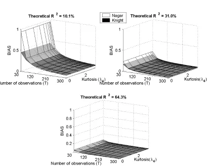
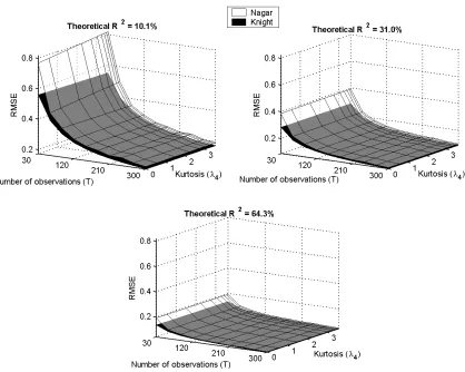
(i) 0.15×i5, whereiis a 5×1 vector of ones, resulting in a theoreticalR2 _{of 10.1%; (ii) 0}_.₃₀_×_i_5, resulting in a theoreticalR2_{of 31.0%; (iii) 0}_.₆₀_×_i_{5, resulting in a theoretical}_R2_{of 64.3%. The first} of these choices can be considered as constituting a case of so called “weak” instruments. To access the impact of the sample size on the bias and the RMSE of the two approximations, we have used different values of T=30,60,90,120, . . . ,300.

The simulation results are illustrated in Figures 2.1 and 2.2, that can be found at the end of this chapter. We discuss these results. Starting with the effect of the sample size, T, the results agree with what one would expect. The higher the sample size, the lower the bias or the RMSE of the IV estimates, irrespective of the method used to calculate them; moreover, as T increases the difference between the two methods decreases and is negligible forT ≥90. Now consider the impact of the first stageR2. As the explanatory power of the instruments increases, there is a significant decrease in the bias and RMSE; no matter which formula is used to calculate the moments. However, the difference between the results based on the approximate (Nagar-type) and exact (Knight-type) formulae is negatively related to R2_{. Finally, we consider the impact of the kurtosis. Recall that} one difference between the formulae for the approximate bias and exact bias is that the former does not depend on the kurtosis but the latter does. Figure 2.1 shows that the kurtosis does not have a significant effect on the exact (Knight-type) bias of the IV estimates. Thus, in the setting studied in this paper, the exact formula for the bias exhibits an invariance to the kurtosis that is enforced by construction in the Nagar-type formula for the approximate bias.4_{. Both the approximate and} exact formulae for the MSE indicate the second moment depends on the kurtosis, but it can be seen from Figure 2.2 that the RMSE hyperplane is almost parallel to the kurtosis axis in all the cases considered. Therefore kurtosis does not appear to have a significant effect on this moment irrespective of whether the approximate (Nagar-type) or exact formulae are used to calculate the second moment.

4

From all the settings studied, only the one with 30 observations and anR2

of 10% shows a slight effect ofλ4 on

(33)

To conclude, we briefly comment the properties of the approximation to the moment matrix to orderT−2 _{presented in Corollary 1. While this approximation is guaranteed to be non-negative for} the case in which the errors are normally distributed (i.e. h= 1), it is not the case for higher values of h in small samples. These results are illustrated in Figure 2.1.1. Calculations reveal that this approximation can yield a negative number within our design when the instruments are “weak”, that is the first stageR2_{= 10}_._{1%. Specifically, we obtain negative numbers at}_T _{= 30 for}_{h >}_{2 and} atT = 35 forh >5, but that the approximation is positive at T ≥40 for all values of h.

(34)

(35)

(36)

(37)

Chapter 3 Edgeworth Expansion of the LM statistic

3.1 Introduction

The Edgeworth expansion can be considered as the most commonly used method for higher order approximations to the distribution of estimators and test statistics. The are two main reasons for the popularity of this methodology. First, it can be viewed as a natural extension of the first order approximation techniques; in fact, the leading term in the Edgeworth Expansion is nothing more than the first order asymptotic approximation. Second, Edgeworth approximations are based on the normal and chi-square distributions which are familiar and easy to use. It is due to these characteristics that, as Rothenberg (1984) suggests:

“Indeed, it [the Edgeworth approximation] is the basis for a general theory of higher-order efficient estimators and tests.” Rothenberg (1984), p. 892

At this point, it is worth noticing that the Edgeworth approximations are not the mostnumerically

accurate. In most applications, there exist curve fitting techniques that yield more accurate numeri-cal results. However, since the Edgeworth expansions lead to general formulae of the distribution of interest, they are very insightful when the researcher wants to know what drives the passage from the finite to the asymptotic sample behavior.

In principle, Edgeworth expansions are very simple; they provide better approximations by taking into account the higher order cumulants of the statistic of interest.

One can identify three main steps that will lead to an Edgeworth expansion of the distribution of a test statistic; these were briefly introduced in the introductory chapter of this research. We will also present them here in more detail.

(38)

Chapter 3. Edgeworth Expansion of the LM statistic

the score functions, as well as to the weighting matrix. The expanded terms are then combined, in order to get the higher order expansion of the test statistic. The key at this point is to express the test in a power series in T−1/2_{, where} _T _{is the sample size, with coefficients that are well defined} random variables. Specifically, assuming that ST is the statistic of interest, we want to get an expansion of the form

ST =X0+T−1/2X1+T−1X2+T−3/2R (3.1)

whereXi,i= 0,1,2, are sequences of random variables with bounded moments asT goes to infinity. If Ris stochastically bounded, the first order approximation to the distribution of ST is the same as the limiting distribution ofX0. The key in the Edgeworth expansion methodology is to use the information inX1andX2to get an improved approximation. To see that, note that the first order asymptotic approximation involves an error of orderOP(T−1/2); takingX1andX2into account will result to an ”improved” error of orderOP(T−3/2).

Thesecond step is to get the characteristic function of the expanded statistic. Using our example, the researcher would have to get the characteristic function ofS∗

T ≡X0+T−1/2X1+T−1X2, where

S∗

T is the second order approximation toST.

Thethird stepis to get the inverse Fourier transform of the characteristic function ofS∗

T. Once this is done, we can get the cumulative and the probability density functions of the expanded statistic,

S∗

T, which provide the Edgeworth approximation to the distribution of theST statistic.

The drawback of this methodology is the complications that might arise when the researcher tries to get the characteristic function and its inverse Fourier transform. These are usually based on long, and quite complicated algebraic expressions, that might not possess a closed form solution. We overcome this problem using an algorithm developed by Cavanagh(1983) and Rothenberg(1988) that bypasses the characteristic function and the inverse Fourier transform step. This algorithm was presented in the introductory chapter; we re-state its main results and notation here for convenience. Suppose the researcher can expand the statistic of interestSin the way defined in equation (3.1) whereX0 has distribution functionF and densityf,Xi,i= 1,2, are sequences of random variables with bounded moments asT goes to infinity, and

p(x)≡E(X1|X0=x), q(x)≡E(X2|X0=x), u(x)≡V ar(X1|X0=x)

are smooth functions ofx. Then, the Edgeworth approximation to the distribution ofS is

P r[ST ≤x]≈F

h

x−_Tp(1/2x) +

2p(x)p0₍_x₎₋₂_q₍_x_{) +}_u0₍_x_{) +}_c₍_x₎_u₍_x₎ 2T

i

(39)

Chapter 3. Edgeworth Expansion of the LM statistic

where

p0(x)≡dp_dx(x), u0(x)≡ du_dx(x), c(x)≡dlog_dxf(x)

This algorithm simplifies greatly the procedure for obtaining an Edgeworth approximation. The only part that complicates the analysis is the calculation of the expectations conditionally on X0 =x. However, this is a rather minor complication in comparison with the inverse Fourier transform of the characteristic function. Thus, we have selected to use this algorithm for our analysis.

3.1.1 The GMM assumptions and notation

Before we proceed with the Edgeworth Expansion, we present the main assumptions of our model.

Assumption 1. The GMM setting that we study is characterized by the following1

1. Population Moment Condition: E(f(ut, ϑ0)) = 0,∀ t,f is defined as

– f :V_×Θ→ <q_{, q <}_∞_{, where}_V_{is the sample space of}_u t.

2. {@ϑ6=ϑ0:E(f(ut, ϑ)) = 0}

3. ut: i.i.d.

4. ϑ0:p×1

5. f(.) :q×1

The notation that we use is as follows.

Definition 2. To simplify the notation, define:

1. g0(ϑ) =E{f(ut, ϑ)}

2. gT(ϑ) =_T1 T

P

t=1

f(ut, ϑ)

3. G0(ϑ) =E[∂f(ut,ϑ)

∂ϑ0 ]

4. GT(ϑ) = _T1 T

P

t=1 f(ut,ϑ)

∂ϑ0

5. ST(ϑ) =var{T− 1 2

T

P

t=1

f(ut, ϑ)}

6. S0(ϑ) = lim T→∞ST(ϑ)

1_{The GMM estimation principle is based on other primitive conditions such as the compactness of the parameter}

Second Order Approximations to GMM Statistics

ABSTRACT

SECOND ORDER APPROXIMATIONS TO

GMM STATISTICS

Biography

ACKNOWLEDGEMENTS

Contents

List of Tables

List of Figures

Chapter 1

Introduction

1.1

Exact Finite Sample Analysis

1.2

Second Order Approximations

1.2.1

The Methodology of Second Order Approximations

1.2.2

The Development of Second Order Approximations

Chapter 2

Evaluating the accuracy of second order

approximations

2.1

Model and assumptions

2.1.1

Comparison with Exact Moments

Chapter 3

Edgeworth Expansion of the LM statistic

3.1

Introduction

3.1.1

The GMM assumptions and notation