Static and Dynamic Influence of a Fluid Droplet on a Soft Deformable Solid.

ABSTRACT

BARDALL, AARON RYDER. Static and Dynamic Influence of a Fluid Droplet on a Soft Deformable Solid. (Under the direction of Michael Shearer).

Here I present an in-depth look at the modeling and analysis of the influence of fluid droplets on soft solids both in static and dynamic cases. The study resides in the field of elastocapillarity,

or the interaction of elastic and capillary influences. The interplay of these two effects leads to

interesting phenomena not limited to those discussed in this thesis. Capillary energy in the form of liquid surface energy, the result of free energy from unbalanced molecular bonds at the fluid phase

interface, influences the geometry of fluids seeking an energy minimizing shape. In the case of soft

solids and fluids interacting, liquid surface energy generates forces which act to alter the shape of the solids introducing strains and elastic energy to the system. In the case of droplets resting

on soft solids, the competition between equilibrium surface and elastic energies results in solid

deformation in the form of a wetting ridge at the three phase triple point, or contact line.

We develop a model describing the influence of a resting droplet on a solid surface. From the

model we obtain quantities such as the displacement of the solid, and resulting geometry of the deformed surface, as well as strains and stresses within the solid. This is done for two dimensional

and three dimensional droplet geometries, as well as the separate scenario of a thin elastic rod being

partially submerged in a fluid.

In the case of the two dimensional droplet geometry, we introduce spatial gradients in solid substrate

properties, specifically the stiffness and solid surface energies. Consequently, equilibrium defor-mations in the solid substrate upon which the fluid rests become spatially asymmetric. The effects

of this asymmetry are investigated as a potential source for inducing droplet motion, which has

been observed experimentally for some scenarios such as solid thickness gradients. We quantify the resulting physical configuration of the system for a given substrate gradient. The absolute difference

in apparent contact angle formed at the front and back of the fluid droplet is used as a benchmark

criterion for the induction of droplet motion. Ultimately we find that given current experimental feasibility, a stiffness gradient is predicted to be insufficient to induce droplet dynamics. In contrast

to this we find that a gradient in surface energy is capable of inducing motion of a fluid droplet over the surface of a soft solid. Dynamic droplet velocities for our feasible scenario are then predicted

© Copyright 2019 by Aaron Ryder Bardall

Static and Dynamic Influence of a Fluid Droplet on a Soft Deformable Solid

by

Aaron Ryder Bardall

A dissertation submitted to the Graduate Faculty of North Carolina State University

in partial fulfillment of the requirements for the Degree of

Doctor of Philosophy

Applied Mathematics

Raleigh, North Carolina

2019

APPROVED BY:

Karen Daniels Mansoor Haider

Ralph Smith Michael Shearer

DEDICATION

BIOGRAPHY

The author, Aaron Bardall, was born in Danville, Pennsylvania on August 31st1991. One thing led to another, and now he resides in Raleigh, North Carolina. According to many who know him, he is

ACKNOWLEDGEMENTS

I would like to acknowledge my family, who have always been there for me. They believed in me even when I did not and I wouldn’t have gotten this far without them. From apples and oranges math for

me and Jared on the swing as kids to being kind, understanding and supportive through every

de-cision I’ve made, I have become who I am because of them and am grateful for their love and support.

In addition I would like to acknowledge all the educators and advisors, especially my commit-tee, who have helped me gain the knowledge and skills necessary to complete this work. Specifically

my advisor Dr. Michael Shearer who has been a pleasure to work with. His support came not only in

his vast knowledge and wisdom, but in his kindness and attention to detail. He was very trusting of me from the start and let me work quite independent from his active research but was always

available to give suggestions and bounce ideas off of throughout the entirety of this project. He has

helped me develop into a mathematician as well as a communicator and I cannot thank him enough.

Alongside Dr. Shearer, Dr. Karen Daniels has been like a second advisor to me throughout my

graduate education. I still haven’t figured out how she does all that she does while providing ex-pertise and attention for each and every one of her students. She is quick to provide personalized

advice from her seemingly endless supply of knowledge and experiences, and I truly believe she

would selflessly drop everything at any time to help someone in need.

I would also like to thank my funding from the National Science Foundation DMS-1517291. Without

TABLE OF CONTENTS

LIST OF FIGURES. . . vi

Chapter 1 Introduction. . . 1

Chapter 2 Background . . . 6

2.1 Elasticity and Continuum Mechanics . . . 6

2.2 Free Surface Boundary Conditions . . . 11

2.3 Contact Line Models . . . 14

Chapter 3 Symmetric Deformation Model. . . 17

3.1 2D Droplet Shape and Fluid Pressure Under Gravity . . . 18

3.2 2D Deformation Model . . . 22

3.3 Error Analysis of 2D Deformation Model . . . 35

3.4 2D Deformation Results . . . 39

3.5 3D Model and Error Analysis . . . 43

3.6 Comparison of Two Dimensional and Axisymmetric Deformations . . . 51

Chapter 4 Deformation of a Partially Submerged Rod . . . 55

4.1 Rod Deformation Model . . . 57

4.2 Results . . . 60

Chapter 5 Substrate Gradients and Asymmetric Deformation . . . 62

5.1 Stiffness Gradient . . . 64

5.2 Surface Energy Gradient . . . 71

5.3 Finite Element Method . . . 73

5.4 Deformation Results for Fourier Transform and Finite Element Methods . . . 79

5.5 Asymmetric Droplet Shape . . . 79

5.6 Elastic Energy and the Total Energy Functional . . . 82

5.7 Results . . . 85

Chapter 6 Energy Dissipation and Droplet Velocity Model. . . 88

6.1 Moving Droplet Model . . . 89

6.2 Elastic Energy of Moving Droplet . . . 93

6.3 Energy Dissipation . . . 96

6.4 Results . . . 97

Chapter 7 Conclusions and Future Directions. . . .100

BIBLIOGRAPHY . . . .103

APPENDIX . . . .107

LIST OF FIGURES

Figure 1.1 Wetting ridge formed by a resting fluid droplet . . . 3

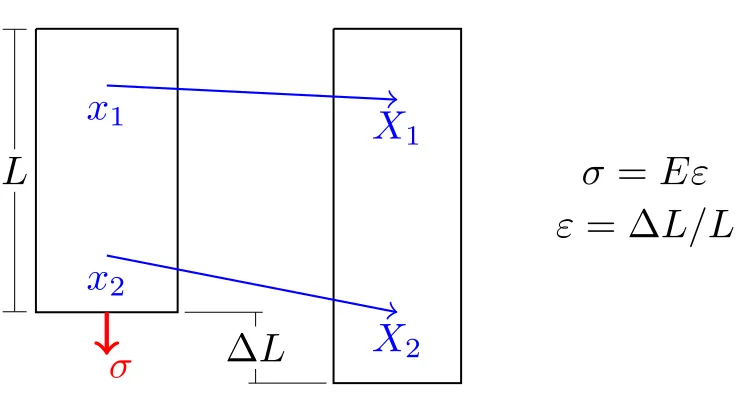
Figure 2.1 Uniaxial loading and deformation of a one-dimensional rod . . . 7

Figure 2.2 Square of elastic material deformed by shear loading . . . 9

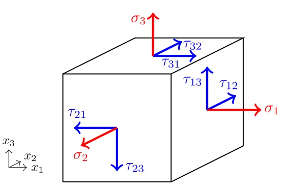
Figure 2.3 Shear and normal loading on a 3d elastic solid . . . 9

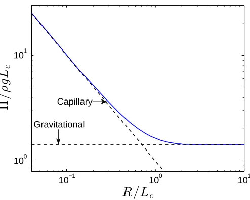
Figure 3.1 Nondimensionalized fluid pressureΠ/ρg Lc as a function of droplet radius for contact angleα=90◦ . . . 21

Figure 3.2 Various size droplet profiles for contact angleα=4π/9 rad under influence of gravity . . . 23

Figure 3.3 Schematic of geometry and forces on a soft substrate influenced by a resting fluid droplet . . . 24

Figure 3.4 Numerical truncation error of deformation at contact line . . . 40

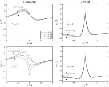
Figure 3.5 Horizontal and vertical displacements of the substrate surface for different tangential contact line models . . . 41

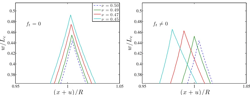
Figure 3.6 Surface deformation near the contact line for example substrate . . . 42

Figure 3.7 Plot of horizontal/radialu and verticalw deformations for both the two dimensional and axisymmetric droplet geometries . . . 53

Figure 3.8 Horizontal deformationufor the two dimensional geometry and radial defor-mationufor the axisymmetric geometry with zero horizontal/radial traction curvature . . . 54

Figure 4.1 Rod geometry experimental setup with submerged rod at different fluid levels 56 Figure 4.2 Axial displacementuz of the PVS gel above the contact line . . . 61

Figure 5.1 Example mesh for FEA simulations . . . 76

Figure 5.2 Test function diagram for FEA analysis . . . 76

Figure 5.3 Deformation results comparison for FEA and transform methods . . . 80

Figure 5.4 Contact angle asymmetry as a function of gradient magnitude in both surface energy and shear modulus . . . 86

Figure 6.1 Velocity prediction for droplets using surface energy gradient . . . 98

CHAPTER

1

INTRODUCTION

Elastocapillarity is the study of the influence of capillary forces on elastic materials. Examples

in-clude capillary rise between elastic sheets[21], smoothing of features on solid slabs[18, 19]and deformation of soft solids by immersion or resting fluids[4, 6, 19, 25, 41]as well as fluid motion

over soft materials[26, 43, 48]. Exploring alternative and novel mechanisms for inducing droplet

motion across soft materials is an emerging subject of interest for the soft matter and fluid dynamics communities. These methods rely on physical substrate configurations for which the droplet profile

becomes asymmetric, subsequently causing a force imbalance driving the droplet to migrate to

a region of lower total energy. Examples of current academic interest include motion induced by gradients in substrate rigidity[8], substrate thickness[43], and substrate pre-strain[7]among others.

Durotaxis, or motion caused by a rigidity gradient, is observed in living cells[31, 43]. In this process, the cells are believed to actively sense and relay changes in stiffness and respond by contracting and

altering cellular shape to migrate to regions of higher stiffness. Though in recent experiments[43],

migration of inorganic fluid is observed to be driven by a gradient in substrate thickness; a physical surrogate for the bulk elastic modulus. In these experiments, the droplets migrate to thicker, less

hard regions of the substrate. This stands at odds with behavior observed by living cells which tend to prefer settling at harder regions of their organic matrix. However, recent computational results

have suggested that fluid migration across a true rigidity gradient may as well be biased toward

fluid-solid-vapor contact line. Further analysis into modes of migration of inorganic fluids may

provide insight into the driving mechanisms for organic cells.

Driving mechanisms for droplet motion across rigid surfaces has been extensively studied. Droplet

motion induced by periodically patterned surface energies[9, 14], thermal gradients[30], and mag-netic fields[12]have been documented to name a few. Like rigid substrates, droplet motion across

soft substrates relies on contact angle asymmetry resulting in a force imbalance inducing migration.

However, additional factors affecting bulk fluid migration across soft substrates include elastic deformations and resulting elastic energy within the substrate as well as bulk energy dissipation

within the substrate. In order to determine conditions for which a fluid droplet will begin to migrate

across a soft surface, the deformation and associated elastic energy must be analyzed.

When a fluid droplet rests on a rigid substrate, surface energiesγat the phase interfaces govern the

equilibrium contact angleθY of the droplet:

γs g −γl s=γl gcosθY (1.1)

This relationship is widely known as Young’s equation, and is the direct result of total surface energy minimization at the phase interfaces. In (1.1), subscripts on surface energy termsγrefer to the

associated interface, i.e.γs g is the surface energy of the solid-gas interface. Young’s equation also

represents a tangential force balance at the triple point, or contact line. The remaining vertical force caused by the liquid-gas interface of the droplet is assumed to be resolved by the ideal rigid solid

substrate for which strains approach zero as stiffness tends to infinity. When the difference in solid

surface tensionsγs g−γl s is positive, the droplet substrate system is termed hydrophilic, and has an

equilibrium Young’s angle ofθY <90◦, whereas if the difference is negative, the droplet substrate

system is hydrophobic with Young’s angleθY >90◦.

For soft solids, non-zero deformations influenced by the capillary forces of the droplet occur within

the substrate introducing elastic energy into the system. This elastic energy competes with the

afore-mentioned surface energy and determination of the equilibrium contact angle via minimization of total system energy becomes more complex. In addition, surface strains affect the solid surface

stresses by the Shuttleworth effect[51, 52]:

Υk=γk+

∂ γk

∂ " (1.2)

thermody-θ

θ

ls

θ

sg

droplet

substrate

air

γ

Υ

ls

_Υ

sg

Figure 1.1Wetting ridge formed by a resting fluid droplet. Solid surface stressesΥbalance surface tension of the contact lineγ. Apparent contact angleθillustrated in blue as the angle the fluid surface forms with the far field horizontal (dashed line), while solid contact anglesθl sandθs g define respectively the angle of the liquid-solid and solid-gas interfaces form with the far field horizontal.

namic property of the two phases meeting at the interface. Surface energy is defined as the work

done to increase the surface area per unit area, while surface stress is defined as the tensile force

per unit width of the surface. For incompressible liquids, these two definitions are equivalent as molecules are free to rearrange absent of any solid structure.

The vertical component of force from the liquid-gas interface pulls up on the substrate creating a wetting ridge (Fig. 1.1). This resulting balance is referred to as Neumann’s triangle[41, 45], where the

solid interfaces now angle downward opposing the upward pull of the droplet edge creating a total

force balance at the contact line. Neumann’s triangle is expressed mathematically by

~

Υs g +Υ~l s+~γ=~0 (1.3)

where solid surface stress vectorsΥ~balance with the surface tension vector~γof the droplet edge. The wetting ridge will form at approximately the size of the elastocapillary length scaleLe =γ/E,

N/m, we find that micro-scale deformations occur at elastic moduli of orderE =O(1−10 kPa). In[42]it is shown that though deformation is negligible in stiff substrates with elastocapillary length Le much less than one micrometer (Le1µm), if the elastocapillary lengthLe is larger than the

atomic length scale, Neumann’s triangle is still formed at the elastocapillary length scale despite

negligible deformation at the visible scale.

For droplets of a similar length scale, these deformations are significant enough to alter the apparent

contact angle, or angle the droplet edge forms with the far field horizontal plane, of the droplet several degrees from Young’s angleθY in (1.1)[41]. While deviation from Young’s angle causes total

surface energy to increase, deviations that reduce the angle with which the liquid-gas interface meets

the solid surface reduces the upward pull of the liquid edge resulting in shallower deformations and strains and thus lower elastic energy. The competition of these two trends generally results

in hydrophobic droplet-substrate systems to have equilibrium angles slightly greater than that

predicted by (1.1), and similarly results in hydrophilic systems having equilibrium angles slightly less than that predicted by (1.1)[8, 41].

When a contact line at the fluid-solid-vapor interface advances or recedes, there are associated advancing and receding contact anglesθa andθr respectively such thatθr ≤θ≤θa, whereθ is

the static contact angle of the droplet. These dynamic contact lines exhibit hysteretic behavior, where by adding volume to the droplet, the contact angle will increase to the advancing angleθ_a,

then the contact line will advance and settle at an equilibrium value. If the additional liquid is then

removed, the contact angle must decrease down to the receding contact angleθrbefore the contact

line recedes[1]. These angles can experimentally be found using the tilted plate method, where

by resting a droplet on a plate and tilting it to an incline such that the droplet begins to migrate,

the contact angles formed at the front and back of the droplet are equivalent to the advancing and receding contact angles respectively[1].

By introducing a gradient in a substrate property such as elastic modulus or surface energy, the apparent contact angle of a resting droplet becomes spatially dependent resulting in contact angle

asymmetry. With enough bias in one direction, the force imbalance generated by the asymmetry can

overcome pinning forces at the contact line and droplet motion is induced. In experiments by Style and Dufresne[43], by comparing to their contact angle theory to their experimental results they

found a contact angle difference of∆θ=θa−θr≈1.8◦was sufficient for water droplet motion over

silicone gel. These results were independent of the droplet size, which is a factor in the equilibrium contact angle of the droplet on a soft surface. This suggests that motion is governed by the relative

The structure of the thesis is as follows. Chapter 2 contains relevant background information on

elastic models and continuum mechanics, as well as the formulation of boundary conditions of a droplet in contact with a free solid surface. These are used to define the model boundary value

problem in the form of model equation and shear and normal stress boundary conditions at the

solid free surface exposed to the droplet. In addition, a discussion regarding current contact line models is included which is important for the general case of a non-trivial tangential contact line

force which is neglected in most models.

Chapters 3 and 4 discuss static models related to the deformation caused by a resting fluid droplet

(Ch. 3) or in a partially submerged rod (Ch. 4). Notably in Ch. 3, a necessary boundary condition is

introduced to accommodate the general loading required of more recent contact line models. In addition in Ch. 4, the quasi-one dimensional submerged rod geometry is analyzed in connection

with the droplet geometry to compare behavior of the contact line force in different geometries.

Experimental results are discussed in Ch. 4, highlighting some of the experimental difficulties nec-essary to overcome in order to determine the nature of the contact line force for the given geometry.

Chapter 5 adapts the two-dimensional deformation model discussed in Chapter 3 to accommodate for gradients in substrate properties, ultimately resulting in contact angle asymmetry. Adopting the

assumptions based on results from[43], we make predictions for when droplet motion is induced based on the relative difference in contact angle values. Ultimately it is shown that despite being

able to cause asymmetry, a stiffness gradient is unlikely to succeed as the sole factor for inducing

droplet motion. However, a gradient in surface energy is a theoretically feasible method for inducing motion over soft substrates.

Chapter 6 discusses methods to predict the resulting speed of droplet motion once sufficiently induced by substrate gradients in Ch. 5. These predictions rely on the balance between system

dissipation and rate that energy is released in the system by migration. Here dissipation occurs

dominantly in the solid, as opposed to the case of a rigid substrate for which dissipation within the fluid is dominant. This extra resistance introduced by the deformation of the solid and associated

energy dissipation slows down the dynamics of droplets over soft solids when compared to motion

CHAPTER

2

BACKGROUND

Here we outline a few topics that will be important throughout the body of the thesis. In §2.1 we

establish formalism in linear elasticity which will be used the model the deformation of our solid substrate. In §2.2 the stress boundary conditions that characterize the surface exposed to the droplet,

or solid free surface, are derived via an energy minimization argument. Through this derivation, the

nature of the contact line force is left ambiguous. A discussion related to current theory presented in[51, 52]as well as experimental conjectures from[28]is presented in §2.3.

2.1

Elasticity and Continuum Mechanics

In a simple uniaxial elastic model depicted in Fig. 2.1, a tensile force applied to a one dimensional

elastic beam induces stress within the beam resulting in a lengthening of the beam. Hooke’s law

relates the applied stressσto the strain"by a material parameter referred to as Young’s modulusE by the following relationship

σ=E" (2.1)

Here, strain is defined as the change in length divided by the original length of the beam ("=∆L/L) and stress is defined as the ratio of applied tensile force over the cross-sectional area of the beam

L

∆

L

σ

x

1

_X

1

x

2

X

2

σ

=

Eε

ε

= ∆

L/L

Figure 2.1Uniaxial loading and deformation of a one-dimensional rod. A stressσis applied tensively to a rod of lengthL, extending the length of the rod by a length∆L. Pointsxi are mapped to corresponding resulting locationsXi=xi+u(xi)in the deformed state.

the rate of change ofuwith respect tox:

"= d

d xu(x) (2.2)

Considering a real three dimensional system, the stretching parallel to the applied force would result

in the contraction of the material in the perpendicular direction. This introduces another material parameter, the Poisson’s ratioν, which relates the perpendicular strain to the axial strain applied to

the rod.

"⊥=−ν"k (2.3)

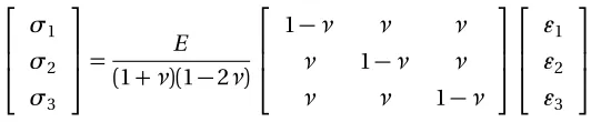
Combining these for loading in three orthogonal spatial dimensions we obtain a generalized Hooke’s

law depending on material parametersE andν:

"11= 1

E σ1−ν(σ2+σ3)

(2.4)

"22= 1

E σ2−ν(σ1+σ3)

(2.5)

"33= 1

E σ3−ν(σ1+σ2)

where strain"i i=∂xiui. This can be put into matrix form:    "11 "22 "33   = 1 E   

1 −ν −ν

−ν 1 −ν

−ν −ν 1

      σ1 σ2 σ3    (2.7)

which can be inverted to give the principal stresses as a function of strain:

   σ1 σ2 σ3   = E (1+ν)(1−2ν)



 

1−ν ν ν

ν 1−ν ν

ν ν 1−ν

      "1 "2 "3    (2.8)

In addition to normal stress-strain relationships derived above, we also are concerned with shear

loading by tangential stresses. For each surface, there are two tangential shear directions as seen in Fig. 2.3 for the six cube faces. We define the shear modulusGby considering a shear stressτapplied to the top of a square in Fig. 2.2, where we define

G =τ∆x

L =τtanφ=τ"s h e a r (2.9)

where the strain"s h e a r =tanφ =∂x2u1. By computing the axial strain from the bottom left to

top right corners and comparing to the definition of the shear modulus, it can be shown that the two moduli are related by equationE =2(1+ν)G. Under multi-dimensional loading, shear forces accomplish three types transformations to the geometry of the elastic solid; these being

shear, dilation and rotation. Shear is captured by the symmetric portion, while rotation by the antisymmetric portion of the matrix

[A]i j =∂xiuj (2.10)

and dilation is represented in both symmetric and antisymmetric portions. Using this, we define

our symmetric strain tensor to be given by

["] ="i j=

1 2 A+A

T

⇒ "i j=

1

2 ∂xiuj+∂xjui

(2.11)

which is self-consistent with the definition of normal strains in (2.4). Using the solution for the

normal strains in (2.8) as well as the stress-strain relationship in (2.9) and by definingτi i=σi, we

obtain the definition of the stress tensor in terms of strain tensor (2.11):

[τ] =τi j τi j=

E 1+ν

”

"i j+

ν

1−2νδi j"k k —

(2.12)

L

∆

x

τ

φ

τ

=

Gε

ε

= tan

φ

Figure 2.2Square of elastic material deformed by shear loading. Stressτapplied along top edge while bot-tom edge is held fixed. The resulting deformation slides the top edge a length∆xand angleφis formed with the vertical dashed line.

x

x

x

σ

τ

τ

σ

τ

τ

σ

τ

τ

Figure 2.3Shear (blue) and normal (red) loading on a 3d elastic solid. Positive orientation of shear stresses

In addition to relating parallel and perpendicular normal strains as in (2.3), Poisson’s ratio is indica-tive of the volumetric dilation of an elastic material under applied pressurep. The bulk modulusK of a material, defined as

K =− V

∆V∆p (2.13)

quantifies the inverse of the volumetric change of material per change in hydrostatic compression ∆p. This tends to infinity for incompressible materials. This modulus can be related to the shear and elastic moduli by relation

2(1+ν)G=E =3(1−2ν)K (2.14)

illustrating thatν=1/2 indicates the solid is incompressible. If the Poisson’s ratio decreases from

ν=1/2 then the bulk modulus in turn decreases representing a larger change in volume∆V per incremental loading∆p, or more total solid compression.

In addition, these moduli from (2.14) relate to the Lamé parametersµandλfrom classical

mechan-ics, which are defined as coefficients for components of the stress tensor:

τi j =2µ"i j+λδi j"k k (2.15)

where by comparing with (2.12), we see thatµis simply the shear modulusG andλ=2Gν/(1−2ν).

Using the derivations from above, we can develop a model describing the motion of a material point

in an elastic solid by the applied stresses to the material. The volume specific force balance equation

is represented by the sum of forces equation

ρ_u~¨_{=∇ ·τ¯+}~_{b (2.16)}

whereρis the mass density,u~is the relative position vector, or displacement vector and~bis the specific body force. With droplet size length scales on the order of the elastocapillary length scale

Le =γ/E =O(10µm), we find that

k~bk ∼ρg L3_e k∇ ·τk ∼γLe (2.17)

This shows in general that gravitational body forces will compete with surface forces only ifLe∼

Lc =

p

γ/ρg, whereLc is the capillary length scale. Under negligible gravitational influence, we

adopt the continuum static equilibrium model to be

Using this with the linear elastic strain tensor (2.15), we obtain (letting∂j =∂xj):

∇ ·τ¯=0 ⇒ ∂jτi j=0 (i=1, 2, 3)

where for spatially constant Lamé parametersµ,λwe have that

2µ∂j"i j+λ∂i"j j=0 (i=1, 2, 3)

⇒µ∂j(∂iuj+∂jui) +λ∂i(∂juj) =0

⇒µ∂j2ui+ (λ+µ)∂i(∂juj) =0

⇒µ∆u+ (λ+µ)∇(∇ ·u) =0

Where upon substituting in our physical parameters we obtain the Elastostatic Navier equations for

static equilibrium of a linearly elastic solid:

(1−2ν)∆u+∇(∇ ·u) =0 (2.19)

Which will be solved for our specific model in later chapters.

2.2

Free Surface Boundary Conditions

Here we establish appropriate surface stress boundary conditions that reflect the influence of a

resting droplet on a deformable elastic substrate. In this section, these boundary conditions will be derived using variational calculus to obtain conditions for a minimum in total system energy, and

applied to our models in future chapters.

Following the work of[27], we seek to define the boundary conditions on the free surface as a

result of a resting fluid droplet. These boundary conditions will define the shear and normal stresses

associated with a resting two-dimensional droplet of radiusRon an elastic substrate which under-goes deformation at the free surface with surface displacement vectoru~(x) =〈u(x),w(x)〉containing the horizontal and vertical displacement of the surface. We will first construct the energy functional

of the system per unit depth with penalties in the form of Lagrange multiplier constraints that restrict the fluid edge to meet with the solid surface at the contact line as well as enforcing constant

cross-sectional areaAof the droplet. Then, taking variations with respect to the droplet heighth(x), contact line locationRand the solid surface profile displacementsu(x)andw(x), we define the shear and normal surface stress boundary conditionsτx z andτz z respectively. Utilizing symmetry,

We define our surface energy functionalEs below:

Es =

Z ∞

0

γs(x)

”p

(1+u0)2+ (w0)2₋₁—_{d x}+ Z R

0

γp

1+ (h0)2_{d x (2.20)}

where the first integral represents the solid surface energy and the second the energy of the liquid-gas

phase. The elastic energy functionalEe l is defined as

Ee l =

1 2

Z Z

Ω

τ·"dΩ (2.21)

which, for the purposes of these calculations, is rewritten using Divergence theorem. The inner

product of the stress and strain tensors is manipulated as follows:

τ·"=〈"x x,"x z〉 · 〈τx x,τx z〉+〈"x z,"z z〉 · 〈τx z,τz z〉

=〈∂xu,

1

2(∂zu+∂xw)〉 · 〈τx x,τx z〉+〈 1

2(∂zu+∂xw),∂zw〉 · 〈τx z,τz z〉 =∇u· 〈τx x,τx z〉+∇w· 〈τx z,τz z〉

=∇ ·(u〈τx x,τx z〉+w〈τx z,τz z〉)

where the last manipulation is a consequence of the equilibrium condition (2.18). Assuming fixed

boundary conditions at the substrate boundaries everywhere except the free surface, we obtain a

simplified energy functional by Divergence theorem:

Ee l =

1 2

Z ∞

0

(uτ_{x z}+w τ_{z z})d x (2.22)

Our total energy functional then becomes the sum of the surface and energy functionals as well as Lagrange multiplier constraint enforcing the triple point at the contact line:

Et o t =Es+Ee l +λc l h(R)−w(R)

+λA

” A−

Z R

0

h(x)−w(x)d x— (2.23)

We take the first variation of the total energy with respect to droplet profile heighth(x):

δEt o t =lim

ε→0

Et o t h(x) +εδh(x)

− Et o t h(x)

ε =lim ε→0 1 ε Z R 0 γp

1+ (h0+εδ_h0)2₋p₁+ (_h0)2_{d x}+λ_{c l}δ_h(_R)₋λ_A ZR

0

δh(x)d x

=lim ε→0 1 ε Z R 0 γp

1+ (h0)2+₂ε_h0δ_h0₋p₁+ (_h0)2_{d x}+λ_{c l}δ_h(_R)₋λ_A Z R

0

where using approximationpa+δ−pa≈δ/2paforaδ, we get

δEt o t =

ZR

0

h0(x) p

1+ (h0)2δh

0_{(x)d x+λ}

c lδh(R)−λA

Z R

0

δh(x)d x

=€

λc l−

h0(R) p

1+ (h0(_R))2 Š

δh(R) + Z R

0

−γκ−λA

δh(x)d x

whereκis the curvature of the liquid surfaceh(x). By definition of Laplace pressure,P =−γκwe obtainλA=P. It also follows thatλc l =γsinθ whereθ is the angle the liquid edge forms with the

horizontal. Following a similar procedure, taking the variation with respect to vertical displacement w(x), we obtain

δEt o t = γl ssinθl s+γs gsinθs g −λc l

δw(R) + Z ∞

0

τz z−γs(x)(~κs·eˆz)

δw(x)d x

+λA

Z R

0

δw(x)d x

whereθl s andθs g are the angle the solid-liquid phase and the liquid-gas phase forms with the

horizontal depicted in Fig. 1.1 and~κs is the curvature of the solid surface. Taking results from the

variation with respect to droplet profileh, we obtain vertical contact line force balance equation

γsinθ=γl ssinθl s+γs gsinθs g (2.24)

as well as definition of normal stress at the free surfaceτz z for locations away from the contact line:

τz z(x) =−P H(R− |x|) +γs(x)(~κs·eˆz)

Incorporating the point loading force of the contact line, we obtain the free surface normal stress

definition by variational principles:

τz z(x) =γsinθ δ(x+R) +δ(x−R)

−P H(R− |x|) +γs(x)(~κs(x)·eˆz) (2.25)

Similarly, by taking variations with respect to contact line locationR and horizontal displacement u(x), we obtain horizontal contact line force balance equation

γcosθ+γl scosθl s=γs gcosθs g (2.26)

and the free surface shear stress definition by variational principles:

whereft is a general tangential point loading at the contact line location, discussed in §2.3. These

stresses (2.25) and (2.27) define the free surface boundary conditions representing the minimum total energy of the resting droplet system. Solving the general model (2.18) in coordination with

these boundary conditions will yield the deformation and associated stresses and strains of the

elastic substrate. In addition, the vertical and horizontal force balances at the contact line (2.24) and (2.26) derived by variational principles validate the Neumman triangle assumption (1.3) in the

absence of the Shuttleworth effect (1.2).

We observe some key features in the stress boundary conditions (2.25) and (2.27), including point

loadings at the contact lines atx=±R, as well as a pressure distribution under the droplet generated by the curvature of the droplet free surface. These stresses are a result of the fluid droplet itself, while the remaining terms involving the solid free surface curvature are a result of the curvature

of the deformed substrate. As will be seen later in Ch. 3, under the assumption of point loading at

the contact line, these traction stresses are crucial to ensure bounded displacements at the contact line location. Though point loading is physically unrealistic, the length scale over which the contact

line applies stress is the atomic length scale of the fluid, which is several orders of magnitude less

than the elastocapillary length scaleL_e=γ/E. Though modeling the contact line as some small, but finite size would alleviate the need to have the solid traction stresses present to resolve unbounded

displacements, our further work will use the point loading model for simplicity, and the inclusion of the solid traction in general only adds to the accuracy of the model.

2.3

Contact Line Models

When considering a fluid contact line with associated surface stressγpulling on the surface of an elastic solid, the strength and orientation of the contact line force determines the resulting

deformation of the solid as a result of the contact line. While for an angleθbetween the surface

normal vector and the vector parallel to the contact line, f_n =γsinθ is well agreed upon as the normal component of force at the contact line, the tangential component ft has been a topic of

debate and interest among soft matter researchers[28, 51, 52].

For droplets resting on rigid substrates exhibiting zero strain, Young’s equation (1.1) defines ana

prioriforce tangential balance. However, Shuttleworth’s equation (1.2) predicts that the solid surface

stresses are dependent on the strain. So for elastic substrates which deform under loading, (1.1) no longer guarantees a force balance in the tangential direction for droplets with contact angle

equivalent to Young’s contact angleθY.

horizontal force balance making the tangential forceft=0, work by[18,52]utilizing thermodynamic

arguments predict a tangential contact line force equivalent to

ft = (Υl s−Υs g)−(γl s−γs g) =

1−2ν

1−ν γ(1+cosθY) (2.28)

which depends on the liquid surface tensionγas well as the Poisson’s ratioν. Notably this predic-tion still yields a tangential force of zero for incompressible substrates, though predicts very large

tangential loading for low values ofν, or highly compressible materials. This aspect of the predicted

formula (2.28) makes it challenging to experimentally test using soft gel materials for which reside near the incompressible limit.

An alternative geometry, where an elastic rod is partially submerged inside a fluid bath, was studied by[28]. In this experiment, small beads were embedded inside the elastic rod to measure the strain

both above and below the contact line. Using the method of virtual work akin to the principal

governing the Wilhelmy plate method for determining surface tensions of liquid,[28]emperically predict a contact line force

ft=γ(1+cosθ) (2.29)

biased toward the liquid, whereθis the angle formed by the liquid meniscus. This equation is similar

to that predicted by[52]in (2.28) without the dependence on the compressibility of the elastic solid.

Using substrate deformation data from [41]for a static droplet, the three contact line models

(2.28), (2.29) andft=0 were examined by[6]. In their simulations, it was shown that (2.29) was an

unrealistic model for a droplet, but did not disprove its application to alternative geometries such as the rod geometry the force model was originally posed in. Furthermore, with the limitation of

the data being from a nearly incompressible substrate, it was unsuccessful in providing insight on whether (2.28) orf_t=0 is the correct model for the droplet geometry.

Furthermore, the previous tangential force models are all designed for fluids which obey Young’s equation (1.1). Under deviation of the contact angleθ fromθY we theoretically predict a contact

line force of

ft=γ(cosθ−cosθY) (2.30)

In order to consider these non-trivial contact line models, adjustments must be made to existing

solution methods in[6, 41]to rectify the displacement singularity occurring due to the point loading approximation. Under linearized curvature, the curvature vector is approximated as completely

normal to the surface which is sufficient to remove the vertical displacement singularity, though is

forceft 6=0. We will show in Ch. 3 that including a horizontal component of the curvature vector,

CHAPTER

3

SYMMETRIC DEFORMATION MODEL

The work presented in §3.1-3.4 of this chapter is taken directly from or paraphrased from previously

published work[4]by myself as well as Dr. Michael Shearer and Dr. Karen Daniels.

On a sufficiently-soft substrate, a resting fluid droplet will cause significant deformation of the

substrate. This deformation is driven by a combination of capillary forces at the contact line and the fluid pressure at the solid surface. These forces are balanced at the surface by the solid traction stress

induced by the substrate deformation. Young’s Law, which predicts the equilibrium contact angle of

the droplet, also indicates ana prioriradial force balance for rigid substrates, but not necessarily for soft substrates which deform under loading. It remains an open question whether the contact line

transmits a non-zero force tangent to the substrate surface in addition to the conventional normal

(vertical) force.

In §3.2 we present an analytic Fourier transform solution technique that includes general interfacial

energy conditions which govern the contact angle of a 2D droplet, for which we solve for the droplet profile and fluid pressure in §3.1. Importantly, we find in §3.3 performing a truncation error analysis

on the inverse transform solutions to the model in §3.2 that in order to avoid a displacement singu-larity at the contact line under a non-zero tangential contact line force, it is necessary to include a

previously-neglected horizontal traction boundary condition. These results are then extended to

are found regarding the displacement singularity at the contact line. Both two dimensional results

and three dimensional axisymmetric results are explored in §3.4 as well as §3.6.

3.1

2D Droplet Shape and Fluid Pressure Under Gravity

The fluid pressureΠand droplet shape are influenced only slightly by the deformation in the sub-strate, which is localized near the contact line. In this section, we determine the pressure and droplet shape by assuming the substrate is rigid and flat. With this assumption, we determine the

relation-ship between the fluid pressureΠand droplet radiusR, and their dependence on surface tension and gravity. We use this then to define the pressure under the droplet used in our boundary value

problem investigated in §3.2 and subsequent solutions.

Gravity influences droplets when the droplet size exceeds the capillary length scale:R>Lc. For small

droplets (R/Lc 1), the droplet surface takes on a circular shape (spherical in three dimensions).

For large droplets, gravity dominates and the droplet flattens out except near the contact line as seen in Fig. 3.2.

The heightf(x)of the droplet free surface above the substrate is determined by minimizing the total energy. The differential gravitational and surface energies are given respectively by

d U_g(x) =ρg f(x) 2

2 d x

and

d Us(x) =γ

Æ

1+f0_(x)2_{d x.}

We then consider the energy cost functionalErepresenting the energy of half the droplet (0≤x≤R), imposing a constant areaArepresenting the amount of fluid in the droplet:

E=

Z

d U_g+d U_s−λ_Ad A+λ_{c l}f(R) = ZR

0

ρg f(x)2/2+γÆ1+f0(_x)2−λ_f(_x)_{d x}+λ

whereλAis a Lagrange multiplier enforcing constant droplet area andλc l is a Lagrange multiplier

enforcingf(R) =0. Computing the first variation with respect to droplet height, we get

δE=lim

ε→0

E(f +εδf)− E(f)

ε =lim ε→0 1 ε Z R 0 ρg

2 (f +εδf) 2

−f2+γÆ1+ (f0_+εδf0₎2₋Æ₁+ (_f0₎2_{d x}

−λA

Z R

0

δf d x+λc lδf(R)

= Z R

0

δfρg f −λA

d x+

ZR

0

γpf0δf0

1+ (f0₎2 d x+λc lδf(R)

= Z R

0

δfρg f −γ f

00

(1+ (f0)2)3/2−λA

d x+δf(R)λc l−γsinα

.

Setting the variationδE to zero we obtain the differential equation

λA=ρg f(x)−γ

f00_(x)

(1+f0(_x)2)3/2 =Πhydrostatic+ΠLaplace=Π. (3.2)

From this we find that the value of the Lagrange multiplierλAis equal to the sum of hydrostatic and

Laplace pressures generated by weight and curvature respectively, whileλc l is equal to the vertical

contact line forceγsinα. This gives us that the fluid pressureΠat the solid surface is constant. In small gravityR/Lc 1, the equation (3.2) gives us that the curvature of the droplet free surface

f(x)is constant, showing that for small droplets the liquid free surface forms a circular cap. It can be shown geometrically that for a circular cap forming a contact angleαwith the horizontal and

projected radiusR, the area of the circular cap is equal toA=R2(αcsc2α−cotα). Using the low gravity approximation, we integrate (3.2) from 0 toRto obtain

Z R

0

Πd x=ΠR= Z R

0 ”

ρg f(x)−γ f

00_(x) (1+f0(_x)2)3/2

—

d x=ρgA

2+γsinα,

giving us an asymptotic approximation of non-dimensionalized pressure for low gravity droplets:

Π

ρg Lc

∼sinαLc R +

αcsc2α−cotα 2 R Lc R Lc 1. (3.3)

shape in terms of the non-dimensionalized pressureΠ/ρg Lc and contact angleα:

Letf0(x) =v(f) ⇒f00(x) =v0(f)f0(x) =v0v

⇒ρg f −γ v

0_v

(1+v2)3/2 =Π

⇒

Z

γ v d v

(1+v2₎3/2= Z

(ρg f −Π)d f

⇒ −γp 1

1+v2=ρg f2

2 −Πf +C

where at f =0 we havef0(f =0) =−tanαgivingC =−γcosα. Solving forv=f0(f)we get

v=d f d x =−

v u t 1 2  _f Lc ‹2 − Π

ρg Lc

f Lc −

cosα −2

−1 (3.4)

⇒

Z f(x)

0 d f v t₁ 2 € _f Lc Š2

−_ρg LΠc

f

Lc −cosα

−2

−1 =

Z x

R

−1d x,

where after nondimensionalization byL_c we obtain

R−x Lc =

Z f(x)/Lc

0

dξ r

1

2ξ2−ρg LΠcξ−cosα

−2

−1

. (3.5)

Enforcing boundary conditionf0(x=0) =0, we know that (3.4) is equal to zero atx=0. From this we obtain condition

f(0) Lc

= Π

ρg Lc

−

v

t€ Π

ρg Lc

Š2

−2 1−cosα. (3.6)

Using upper bound from (3.6), we search for nondimensionalized pressureΠ/ρg Lc which satisfies

(3.5) atx=0 using a bisection algorithm, then with the pressure defined we solve (3.5) implicitly for droplet profilef(x). In Fig. 3.1, we plot the curve of such values for a contact angle ofα=90◦ obtained numerically from (3.5), (3.6) for specifiedR/Lc.

We further manipulate (3.5) to analytically solve for the asymptotic behavior of the

nondimen-sionalized pressurep =Π/ρg Lc asR/Lc → ∞. Enforcing that (3.6) is real valued, we define the

minimum pressure to bep₀=2 sin(α/2)for which we obtain cosα=1−p2

10−1 100 101 100 101

R/L

Π

/

ρ

g

L

Figure 3.1Nondimensionalized fluid pressureΠ/ρg Lc as a function of droplet radius for contact angle

α=90◦. The capillary limit represents the Laplace pressure which decays inversely to the droplet radius

R, while the gravitational limit represents the hydrostatic pressure limit generated by the fluid with depth equivalent to the equilibrium height of the fluid droplet asR→ ∞.

variablesη=p−ξwe obtain

R Lc

(p) = Z p−

q p2_−p2

0

0

dξ Ç

1

2ξ2−pξ−cosα −2

−1

= Z

q p2_−p2

0

p

−dη Ç

1

2(p−η)2−p(p−η) + 1 2p02−1

−2

−1

= Z p

q p2_−p2

0

1−12 η2−(p2−p02)

Ç

1− 12 η2−(p2−p02)

−12 dη

Expanding the integrand aboutζ=qη2₋(_p2_−p2

0), the integrand becomes

1−12 η2−(p2−p02)

Ç

1− 12 η2−(p2−p02)

−12

= 1−

1 2ζ2 Ç

1− 12ζ2−1 2=

1−12ζ2

ζq1−14ζ2

∼1 ζ+O(ζ)

And we obtain estimate asR/Lc→ ∞:

R Lc

∼

Z p

q p2_−p2

0

dη q

η2₋(_p2_−p2 0)

=cosh−1q p p2_−p2

0

Solving algebraically forp we obtain

cosh2 R L_c ∼

p2 p2_−p2

0

⇒ p∼p0coth R L_c

asR/L_c→ ∞and we get

Π

ρg Lc ∼

2 sin(α/2)coth R Lc

R Lc

1. (3.8)

which asymptotes atΠ/ρg Lc=2 sin(α/2).

Fig. 3.1 illustrates that for droplets with projected radiusR ®0.3Lc, the Laplace pressure

dom-inates hydrostatic pressure and a circular cap approximation for the droplet shape is accurate. Past

the transition region 2Lc®R, we observe the hydrostatic pressure dominate the Laplace pressure

and the droplet shape flattens out tof(x)≈f(0) =2Lcsin(α/2)everywhere except in the vicinity of

the contact line. While for small droplets, the large Laplace pressure is significant in influencing

deformation, as droplet size increases this pressure reduces in magnitude and negligibly affects the deformation.

Plotted in Fig. 3.2 is the droplet shape profile for a contact angle ofα=4π/9 radians for droplets of various sizes. We see that for small dropletsR/Lc 1 that the droplet profile closely matches that of

the circular cap approximation and begins to deviate from this limit as the ratioR/Lc approaches

and exceeds 1.

3.2

2D Deformation Model

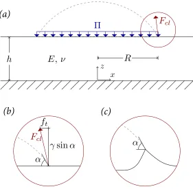
We consider the two dimensional droplet outlined in §3.1 resting on a solid substrate, depicted schematically in Fig. 3.3, with width 2R and resting on the free upper surface of a solid elastic

substrate. In the reference configuration, the substrate is taken to be fixed on the bottom surface

z =0, to have infinite extent, and to have constant thicknessh. The elastic modulus of the substrate is denoted byE, and Poisson’s ratio byν. The contact line introduces a vertical forceγsinαand a tangential forceft which cause significant deformation in a neighborhood of the contact line,

depicted in Fig. 3.3(c). The fluid pressureΠin the droplet acts at the substrate interface to compress the substrate below. In this chapter, we quantify these influences and describe the deformation of

the substrate.

The model depends largely on the formulation of boundary conditions at the free surface of the

0 0.2 0.4 0.6 0.8 1

x=R

0 0.2 0.4 0.6 0.8 1

f

(

x

)

=

R

R=Lc= 0:1

R=Lc= 0:3

R=Lc= 1

R=Lc= 3

R=Lc= 10

R=Lc= 30

Figure 3.2Various size droplet profiles for contact angleα=4π/9 rad. As the size of the dropletR/Lc increases, we see the droplet profile transition from the circular cap approximation (black dotted line) to a flat profile shape in the extreme limit ofR/Lc.

the liquid solid interface and the solid-gas interface between the substrate and air. The effect of the

droplet is expressed solely through the surface stress at the substrate surface and through the

pres-sureΠ. Once these are quantified, the droplet is effectively removed from the subsequent analysis.

To determine the shape of the substrate free surface, we formulate a boundary value problem for the elastic displacement within the substrate. It is convenient to use Eulerian coordinates(x,z), shown in Fig. 3.3. in which the substrate free boundary is located atz=h in the reference configuration. The displacementu~of the substrate is then represented in two components by

~

u(x,z) =u(x,z)eˆx+w(x,z)eˆz, −∞<x<∞, 0<z <h, (3.9)

where ˆex, ˆez are unit vectors in the coordinate directions. The displacement is defined relative to

the reference configuration, mapping the reference configuration to the static deformed substrate configuration:

x,z7→ x+u(x,z),z+w(x,z).

The elastostatic Navier equations

h

E

,

ν

R

z

x

Π

F

(a)

α

F

f

γ

sin

α

(b)

α

(c)

Figure 3.3Schematic of geometry and forces. (a) Reference configuration showing horizontal substrate layer and droplet surface (dashed). Fluid pressureΠand contact line forceFc l act on the solid substrate with elastic modulusE and Poisson ratioν. (b) Blow-up at the contact line showing the effective contact angleα, and contact line forceFc l that includes a non-zero tangential stress componentft. (c) Deforma-tion of the substrate free surface caused by capillary forces.

derived in Ch. 2 express force balance within the substrate. Hereνis the Poisson ratio of the substrate,

where incompressible solids have a Poisson ratio ofν=1/2. In two dimensions, the strain"and

stressτare represented by 2×2 matrices with components,

"i j=

1 2

”∂u_i

∂x_j +

∂uj

∂x_i —

(3.11)

and

τi j =

E 1+ν

”

"i j+

ν

1−2νδi j "11+"22 —

(3.12)

Fixed boundary conditions are set at the solid surface z =0, where displacement is assumed to be zero:

(u,w)|z=0= (0, 0). (3.13)

The effect of the droplet on the substrate is quantified by defining the shear stressτx z and normal

stressτ_{z z} at the free surfacez=hderived in Ch. 2:

τx z|z=h=ft δ(x+R)−δ(x−R)

+Υ(x)~κs(x)·eˆx

(3.14)

τz z|z=h=γsinα δ(x+R) +δ(x−R)

−ΠH(R− |x|) +Υ(x) ~κs(x)·eˆz

(3.15)

where ft is the tangential point loading at the contact line,γsinαthe normal point loading at the

contact line,Πthe pressure distribution calculated in the previous section,Υ(x)being the solid surface stress,~κs(x)the curvature of the solid surface, andδ(x)andH(x)being the Dirac delta

and Heaviside distributions respectively. We assume that the contact angleαis equivalent to the

equilibrium Young’s angleθY.

By considering the general curvature vector instead of just the linearized vertical component,

as done in previous work[6, 19, 41], we will show that the strain is bounded at the contact line in the horizontal as well as the vertical directions under a general contact line force. The solid surface

stress is represented as the piecewise constant function

Υ(x) =Υ_{s g} +∆ΥH(R− |x|), with ∆Υ=Υl s−Υs g. (3.16)

The vectorr~(x) =〈x+u,w+h〉|z=hparameterizes the substrate free surface. Then the curvature

vector is given as

~κs(x) =

(1+∂xu)∂x xw−∂x xu∂xw

(1+∂xu)2+ (∂xw)2

2 (−∂xw)eˆx+ (1+∂xu)eˆz

z=h. (3.17)

The conventional model assumes no tangential contact line force (ft=0). In this case, which

simpli-fies the model, there is a bounded solution at the contact line. The inclusion of an approximation

to the horizontal component of curvature in (3.14), (3.15) is expected to improve the fidelity of the solution by reconciling for the previously neglected horizontal traction force. In the general model

(ft6=0), the inclusion of the horizontal curvature approximation ensures a bounded solution, which

otherwise would experience a logarithmic singularity at the contact line. In the generalized model,

this tangential contact line forceft arises due to the difference between surface stress and surface

conventional model as well as the form proposed by[51, 52]discussed in Ch. 2:

ft=

1−2ν

1−ν γ(1+cosα), (3.18)

It is useful to express the displacement vectoru~(x,z)in terms of a potential functionΨ. To do this, we define a Galerkin vectorG=Ψ(x,z)eˆ_z [6, 39], and define

~

u(x,z) =2(1−ν)∆G− ∇(∇ ·G). (3.19)

By manipulating (3.19) and substituting into the Elastostatic Navier equations (3.10) we obtain:

~

u=〈−∂x zΨ, 2(1−ν)(∂x xΨ+∂z zΨ)−∂z zΨ〉

=〈−∂x zΨ, 2(1−ν)∂x xΨ+ (1−2ν)∂z zΨ〉

⇒∆u~=〈−∂x x x zΨ−∂x z z zΨ, 2(1−ν)∂x x x xΨ+ (3−4ν)∂x x z zΨ+ (1−2ν)∂z z z zΨ〉

and

∇(∇ ·u~) = (1−2ν)∇(∂x x zΨ+∂z z zΨ) = (1−2ν)〈∂x x x zΨ+∂x z z zΨ,∂x x z zΨ+∂z z z zΨ〉

which gives us by plugging in to the elastostatic Navier equations

⇒(1−2ν)∆u~+∇(∇ ·u~) = (1−2ν)〈0, 2(1−ν)∂x x x xΨ+2∂x x z zΨ+∂z z z zΨ

〉=〈0, 0〉

From this we obtain that the potential is biharmonic:

∆2_{Ψ(x,z) =0 (3.20)}

We then obtain displacements and stresses in terms of potential functionΨ:

u = −∂_{x z}Ψ, (3.21a)

w = 2(1−ν)∂x xΨ+ (1−2ν)∂z zΨ, (3.21b)

τx z =

E

1+ν((1−ν)∂x x xΨ−ν∂x z zΨ), (3.21c)

τz z =

E

1+ν((2−ν)∂x x zΨ+ (1−ν)∂z z zΨ). (3.21d)

One advantage of this potential functionΨis that its definition allows for direct calculations involving incompressible solids where the Poisson’s ratioν=1/2, which is a good approximation for nearly

incompressible soft materials such as PDMS or hydrogels. Using the definitions (3.21) it is shown

we see the trace of the strain tensor is proportional to denominator(1−2ν):

"k k="x x+"z z=∂xu+∂zw= (1−2ν)∂z∆Ψ

and we obtain stress tensor

τi j=

E 1+ν

"i j+ν∂z∆Ψδi j

.

We then manipulate the biharmonic equation (3.20) using a Fourier transform and obtain a

sys-tem of equations to solve for the transformed potential. The Fourier transform is conducive to the

cartesian coordinate representation of our two dimensional droplet, whereas a Hankel transform is appropriate in axisymmetric coordinates for the three dimensional droplet[6]and will be discussed

later in §3.5. The surface displacements are recovered by truncating the inverse transform at a

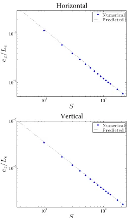
large wave numberS. The asymptotic behavior of the error in this approximation show that the displacement singularity is completely regularized when using both traction boundary conditions.

In this chapter, we define the Fourier Transform pair for a functionf(x,z):

Ff(x,z)=fˆ(s,z) =p1

2π Z ∞

−∞

f(x,z)ei s xd x,

f(x,z) =F−1fˆ(s,z)=_p1 2π

Z ∞

−∞ ˆ

f(s,z)e−i s xd s (3.22)

wheres is the wavenumber. This transform has derivative propertyF[f0(x)] =−i sfˆ(s). Applying the forward transform (3.22) to the biharmonic potential equation (3.20), we obtain

F∆Ψ(x,z)=F∂x x x xΨ+2∂x x z zΨ+∂z z z zΨ

= (−i s)4Ψˆ+ (−i s)2∂z zΨˆ+∂z z z zΨˆ

=

d4 d z4−2s

2 d2 d z2+s

4

ˆ Ψ

=

d2 d z2−s

2 2

ˆ Ψ=0

which has general solution for the transformed potential:

ˆ

Ψ(s,z) = A(s) +s z B(s)cosh(s z) + C(s) +s z D(s)sinh(s z). (3.23)

conditions (3.13), we calculate relationships between these Fourier coefficients:

u(x, 0) =0⇒ Fu(x, 0)=0

⇒ F−∂x zΨ x, 0)] =0

⇒i s∂zΨ(ˆ s, 0) =0

⇒i s2” A(s) +s z B(s) +D(s)sinh(s z) + C(s) +s z D(s) +B(s)cosh(s z)—

z=0=0

⇒i s2 C(s) +B(s)=0

⇒B(s) =−C(s)

and

w(x, 0) =0⇒ Fw(x, 0)=0

⇒ F2(1−ν)∂x xΨ(x, 0) + (1−2ν)∂z zΨ(x, 0)

=0

⇒ −2(1−ν)s2Ψ(ˆ s, 0) + (1−2ν)∂z zΨ(ˆ s, 0) =0

⇒ −2(1−ν)s2”A(s) +s z B(s)cosh(s z) + C(s) +s z D(s)sinh(s z)—

z=0+ (1−2ν)s2”A(s) +s z B(s) +2D(s)cosh(s z) + C(s) +s z D(s) +2B(s)sinh(s z)—

z=0=0

⇒ −2(1−ν)s2A(s) + (1−2ν)s2 A(s) +2D(s)=0

⇒s2 −A(s) +2(1−2ν)D(s)=0

⇒A(s) =2(1−2ν)D(s)

These expressions are substituted into (3.23) where the transformed potential ˆΨis now an expression involving two unknown Fourier coefficientsC(s)andD(s). After nondimensionalizing lengthsx andzsuch thatx=±1 corresponds to the contact line location andz=h˜ =h/Ris the substrate free surface, Fourier coefficientsC(s)andD(s)are determined from the two stress boundary conditions (3.14), (3.15) as follows. The convolution identityFf(x)g(x)=Ff(x)∗ Fg(x)/p2πis used throughout.

Transforming the shear stress boundary condition (3.14) we obtain

Fτx z(x,h)

=Fft

R δ(x+1)−δ(x−1)

+FΥ(x)~κs(x)·eˆx

= ft

RF

δ(x+1)−δ(x−1)+Υs gF

κs(x)·eˆx

+p∆Υ

2πF

H(1− |x|)∗ Fκs(x)·eˆx