A Statistical Characterization of the Genetic Structure of Populations

ABSTRACT

SAMANTA, SUVAJIT. A Statistical Characterization of the Genetic Structure of Pop-ulations. (Under the direction of Bruce Spencer Weir).

In a random mating population the second order descent measure which is also known as coancestry coefficient (θ) characterizes population structure. This struc-ture provides information regarding the history of a population. Characterizing inbred populations, however, requires third (γ) and fourth order (δ and ∆2,2) descent mea-sures. These descent measures are also used to find different expressions in DNA profile matching. In literature there are several estimators for second order descent measure but no estimator exists for the higher order descent measures. In this research we find estimators for second and third order descent measures using a Method of Moments approach and a Probabilistic approach. Simulation studies show that our new esti-mators for second order descent measure are more accurate than the existing moment estimators while the estimators for third order descent measure are stable in terms of bias and standard error. We also derive the sampling properties of our estimators. Later, we relax the constraint that the descent measures have the same value in dif-ferent populations and find estimators for population-specific θ and γ. We implement our methods on HapMap SNP data and find the estimates of the descent measures for the human populations.

The expressions for genetic parameters generally depend on the coancestry coeffi-cient (θ) and become very simple when the coancestry coefficient is zero. In this thesis we propose different testing techniques for testing H0 : θ = 0 vs. H1 : θ > 0 for ran-dom population. For small sample sizes we propose a parametric bootstrap test that has higher power than the non-parametric bootstrap test proposed by Dodds (1986). When the sample sizes are large we find an asymptotically chi square test that works for any number of allelic forms in a particular locus. For more than two alleles per locus our test is better than the asymptotic test proposed by Li (1996). We implement our testing procedures on HapMap SNP data and find that the coancestry coefficient for humans is strictly positive.

gener-alization of Wright’s inbreeding coefficient. The two-locus identity is a useful parameter in predicting the joint ancestry of pair of loci which is frequently used in mapping stud-ies and in finding variances and covariances of quantitative traits. Weir and Cockerham (1969) extended the inbreeding coefficient concept for two loci to evaluate a measure of identity of descent for genes at each of two linked loci. In this research we show that the two-locus descent measures are not estimable but we can estimate the product of link-age disequilibrium and two-locus descent measures. We find the estimators of different components of the two-locus descent measures multiplied with linkage disequilibrium using a Method of Moments approach. We use haplotype data.

A STATISTICAL CHARACTERIZATION OF THE GENETIC STRUCTURE OF POPULATIONS

by

Suvajit Samanta

A dissertation submitted to the Graduate Faculty of North Carolina State University

in partial fulfillment of the requirements for the Degree of

Doctor of Philosophy

STATISTICS

Raleigh 2006

APPROVED BY:

Dr. Subhashis Ghoshal Dr. Dahlia Michelle Nielsen

Dr. Eric Alan Stone Dr. Bruce Spencer Weir

DEDICATION

BIOGRAPHY

ACKNOWLEDGEMENTS

First, I would like to express my gratitude to my advisor Dr. Bruce Weir. I am espe-cially grateful for his incredible patience and understanding. Through my interactions with him I have learned a great deal not only about research but also about life. I am grateful for the opportunity to work with him.

I wish to express my appreciation to my committee members, Dr. Subhashis Ghoshal, Dr. Dahlia Nielsen, and Dr. Eric Stone for their valuable input and ser-vice. These wonderful people helped me in both academic and non-academic matters. I would like to acknowledge Dr. Sujit Ghosh for his guidance and help. I also would like to thank Dr. Keneth Olsen and Dr. Barbara Schaal for kindly responding to my request for their previously published data set.

I thank everyone at Statistics Department and Bioinformatics Research Center for their friendship and help through my studies. I would like to thank Prasenjit Kapat for always being ready to help with any statistical problems specially with statistical computing and R, Sunil Suchindran for helping me with any genetics problems, and Arin Chaudhuri for his invaluable help and guidance during the first two years of my studies. My doctorate would have been impossible without my room mates and Indian friends who helped in in all possible ways.

TABLE OF CONTENTS

List of Tables viii

List of Figures x

1 Review 1

1.1 Introduction . . . 1

1.2 F-statistics . . . 2

1.3 Descent Measures . . . 4

1.4 Heterozygosity . . . 9

1.5 Wright-Fisher Model . . . 10

1.6 Theoretical Values of Descent Measures . . . 11

1.6.1 No Mutation . . . 11

1.6.2 Both-Way Mutation . . . 14

2 Estimation of Decent Measures 18 2.1 Introduction . . . 18

2.2 Replication of Evolution . . . 22

2.3 Data . . . 23

2.4 Review of Existing Estimators of θ . . . 24

2.4.1 Method of Moments Estimator . . . 24

2.4.2 ML Estimator Based on Normal Distribution . . . 25

2.4.3 Bayesian Estimator . . . 26

2.5 New Estimators of θ and γ . . . 27

2.5.1 Method of Moments Estimator . . . 27

2.5.2 Estimators with Probabilistic Interpretation . . . 31

2.6 New Estimators of Population-specific θ and γ . . . 34

2.6.1 Estimators with Probabilistic Interpretation . . . 34

2.6.2 Method of Moments Estimator . . . 37

2.7.1 Weir-Cockerham’s Estmator . . . 44

2.7.2 New Moment Estimator of θ . . . 46

2.7.3 New Moment Estimator of γ . . . 50

3 Testing Hypotheses about θ 53 3.1 Introduction . . . 53

3.2 Review on Testing Procedure . . . 54

3.3 New Testing Procedures . . . 60

3.3.1 Parametric Bootstrap . . . 60

3.3.2 Large Sample Test . . . 61

4 Two Loci 65 4.1 Introduction . . . 65

4.2 Two-Locus Parameters . . . 67

4.3 Theoretical Values of the Parameters . . . 68

4.4 Notation . . . 70

4.5 Data . . . 71

4.6 Identifiability Problem . . . 73

4.7 Moment Estimator of Θ1_D kl and 1ΘDkl . . . 75

4.8 Moment Estimator Of 1Θ11Dkl and 1Γ11Dkl. . . 76

4.9 Ancestral Population is in Linkage Equilibrium . . . 79

5 Variance of Heterozygosity 82 5.1 Introduction . . . 82

5.2 Estimation of Variance of Heterozygosity . . . 85

5.2.1 A Linear Model Approach . . . 87

5.2.2 A Generalized Linear Mixed Model Approach . . . 88

6 Simulation Studies 93

6.1 Introduction . . . 93

6.2 Pure Drift Model . . . 94

6.3 Both-way Mutation Model . . . 98

6.4 Results . . . 99

6.5 Application on HapMap Data . . . 123

6.6 Application on Another Published Data set . . . 126

7 Discussion 132

Appendices 146

A The Relations between the Moment and the Probabilistic Estimators147

B Derive the Simpler Form of a Test Statistic 149

LIST OF TABLES

1.1 Possible arrangements for different alleles . . . 6 1.2 Inbreeding coefficients for two, three and four alleles and their relation

with descent measures under a random mating population . . . 8

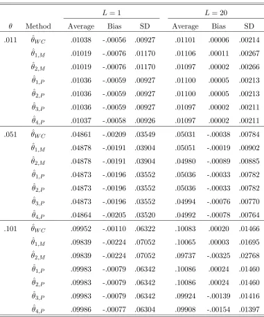
3.1 The contingency table for χ2 _{test when there are two alleles A and a . 56} 6.1 Different estimators of θ. Parameters: s = 2; p = (0.7,0.3); L = 1,20;

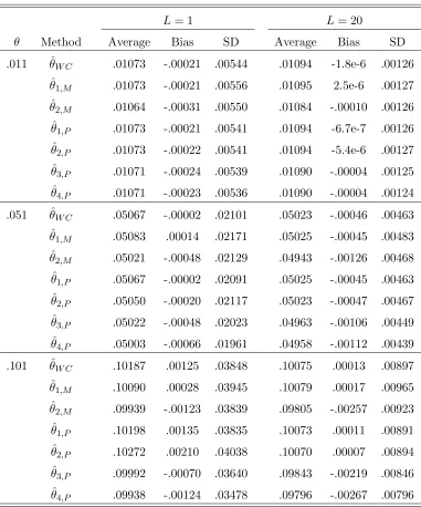
The data is generated with a pure drift model. . . 111 6.2 Different estimators of θ. Parameters: s= 4; p= (0.25,0.25,0.25,0.25);

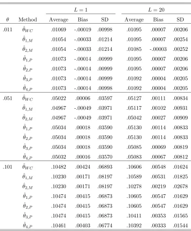
L= 1,20; The data is generated with a pure drift model. . . 112 6.3 Different estimators of θ. Parameters: s = 2; p = (0.7,0.3); L = 1,20;

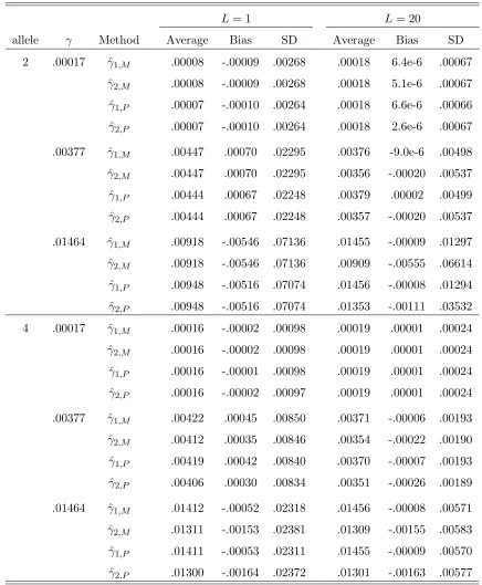
The data is generated with a both-way mutation model. . . 113 6.4 Estimators of γ. Parameters: L= 1 and 20;s = 2 and 4; p= (0.7,0.3)

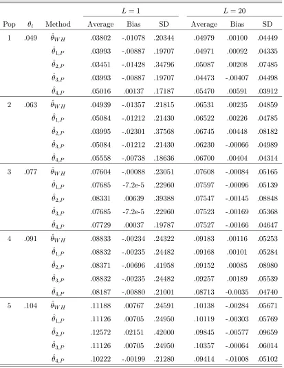
and (0.25,0.25,0.25,0.25); The data is generated with a pure drift model.114 6.5 Estimators of θi. Parameters: s = 2; p= (0.7,0.3);L= 1 and 20; The

data is generated with a pure drift model. . . 115 6.6 Estimators of θi. Parameters: s = 4; p = (0.25,0.25,0.25,0.25); L =

1,20; The data is generated with a both-way mutation model. . . 116 6.7 Different estimators ofγi. Parameters: s= 4;p= (0.25,0.25,0.25,0.25);

L= 1,20; The data is generated with a pure drift model. . . 117 6.8 Estimates of two-locus descent measures. Parameters: s = 2; p = (0.7,

0.3); The data is generated with a pure drift model. . . 118 6.9 Estimates of two-locus descent measures. Parameters: s= 4;p = (0.25,

0.25, 0.25, 0.25); The data is generated with a pure drift model. . . 119 6.10 The comparison between the empirical powers of newly proposed

6.11 The comparison between the empirical powers of newly proposed chi square test statistics with Li’s test procedure. We consider equal sample sizes for different populations. The data is generated with a pure drift model. . . 121 6.12 Relationship between several different expressions for the variance of

heterozygosity ( ˜Hi). The terms given are heterozygosity, within and total-population standard deviation of observed heterozygosity, single-locus and empirical approximation of standard deviation of heterozy-gosity. The data is generated from 10 populations at 5 independent loci using a Pure drift model. . . 122 6.13 Chromosome lengths and numbers of markers segregating in all

popula-tions . . . 125 6.14 Estimates of population-specific and overall θ and overall γ based on

single-locus and 5-Mb window for HapMap data . . . 127 6.15 Relationships between different expressions for the variances of ˜Hi for

the pooled data obtained from Olsen data set . . . 130 6.16 Relationships between different expressions for the variances of ˜Hi for

LIST OF FIGURES

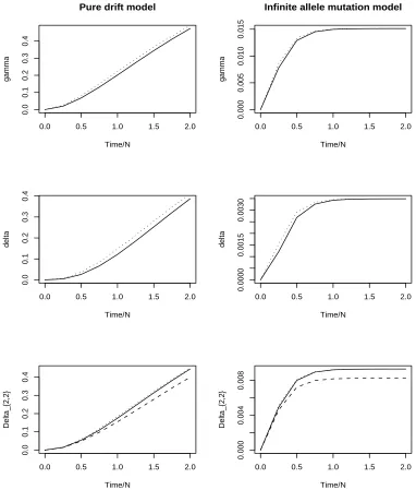
1.1 γe, δe, ∆e from equations (1.21) (dotted line) and γn, δn, ∆2,2,n from

equations (1.17) (dashed line) compared to exact value of γ, δ, ∆2,2 under a pure drift model and a both-way mutation model (same as an infinite allele model). N = 5,000 and the mutation rate of the both-way mutation model is 0.0005. . . 17

Chapter 1

Review

1.1

Introduction

This research covers two different subjects. One is related to decent measures and the other one is related to heterozygosity. The first part of the research evaluates the adequacy of Dirichlet and Normal distribution for allele frequencies. Then it covers different estimation procedures for decent measures and finds the sampling properties of the estimators. It also covers different procedures for testing hypotheses about the coancestry coefficient including the analysis of variance and parametric bootstrap method. The second part of the research is related to the sampling properties of the estimator of heterozygosity. The motivation and the goal of the different parts of the research will be described separately in the following chapters.

The population structure can be characterized by two different set of parameters (i)

the population structure. The F-statistics and descent measures are conceptually the same under a random mating system. This research is developed under a random mating population. It uses descent measures to characterize a population’s structure. Geneticists are interested in finding the genetic distance between different populations. This distance involves the knowledge of decent measures. In current forensic studies, decent measures become a tool to characterize the DNA profile matching.

Heterozygosity and gene diversity are basic tools for summarizing the pattern of genetic variation in a group of populations. Characteristics of population genetic vari-ation are of key interest in studies of evolution. The amount of varivari-ation present in a population or species determines the capacity of the heritable change of the group. So the estimate of heterozygosity and gene diversity can be very helpful descriptive measures for populations. To know the population better we also need to find the sampling properties such as bias and variance of these estimators.

In this chapter we introduce all the necessary parameters in detail and review the development of these parameters. Then we discuss different population models that will be used in this research. We also draw conclusions about the relationship between different parameters for a random mating population under different mutation models.

1.2

F

-statistics

The population structure is frequently modeled as associations between alleles. These associations can occur on different levels, and to different extents. This association can occur within individuals, between individuals within a population, and between indi-viduals in different populations. The inbreeding coefficient was first proposed by Wright (1921). Later Wright extended his work for hierarchial population model and intro-duced three F-statistics, FIS, FST and FIT which represent three different levels of association (Wright, 1951). These F-statistics can be defined as the correlations be-tween alleles sampled from different levels in the population. The subscripts of the

S stands for sub-populations andT for the total population. FST is commonly referred to as the coancestry coefficient, and it measures the degree of relationship, between the individuals within populations relative to the amount of relationship found in the total population. FIT is called the fixation index because it measures the progress of a neutral locus towards fixation to a single allele under the influence of random genetic drift. FIS measures the amount of departure from the Hardy-Weinberg equilibrium of a population.

Cockerham (1969) renamed theF-statistics asf =FIS,θ =FST andF =FIT in his work. This is done to reduce confusion between theF-statistics and theF distribution. He also wanted to emphasize that these measures are population parameters rather than statistics that are functions of observed data. Since these three parameters, f, θ

and F are correlation between alleles, the range of these parameters is from ₋1 to 1. Inbreeding within population occurs when some particular individuals are more related to each other than the relatedness of a random set of individuals from the total population. Two factors contribute to the total amount of inbreeding in a set of populations. Generally one factor contributes to θ; the other factor contributes to f. The random genetic drift results in differences among sub-populations that descended from a founder population which contributes to the value of θ. For a single population, drift can be described as the inbreeding coefficient. The assortive mating within populations increase the value of f. Both the factors, θ and f can increase the amount of inbreeding of the whole group of populations. The total inbreeding coefficient, F, is related toθ and f and the relation is (Weir, 1994)

F =f +θ(1₋f).

1.3

Descent Measures

Descent measures are parameters that also describe the association among alleles. The development of descent measures is based on the concept of identical by descent (ibd). A set of alleles is called identical by descent if all the alleles are descended from a common allele in some ancestral population and no allele has gone thorough mutation. The definition of ibd explicitly implies that the ibd alleles have the same allelic form. The probability that two or more alleles are identical by descent is called descent measures. For two allele case, the alleles can come from one individual or two different individuals in the same population. Mal´ecot (1948) defined the descent measures for two alleles. He used the same notations asF,θandf for defining three different descent measures. Since these parameters are probabilities of different events, the value of these parameters is always non-negative. Mal´ecot (1948) defined the three parameters

F = Esub−pop

P r(Two alleles from an individual are ibd), (1.1)

θ = Esub−pop

P r(Two alleles from two individuals within a population are ibd), (1.2)

f =P r(Two alleles from an individual in a population are ibd), (1.3)

where “Esub−pop” is to mean that the parameters are defined for random population

set up. In this set up we have more than one populations and every population has evolved from the same founder population. In our set up, F and θ are parameters for the random population set up and provide information about the history of the populations. On the other hand, the parameter f is defined for a single population.

Although the two definitions are different theoretically, the definitions are conceptually equivalent for a random mating system. When random mating occurs within the popu-lation, the proportion of heterozygosity reduces over time and the correlation between two alleles is always positive. This implies that the parameters defined by Wright take positive values under a random mating system. According to Wright’s definition, the coancestry coefficient, θ, measures the differentiation between populations. If the value of θ (defined by Wright) is negative then, two alleles are more related if they are from different populations than if they are from same population. If the populations have been isolated since the base population and mate randomly within sub-populations, differentiation between sub-populations will increase over time. Therefore, the value of

θ (defined by Wright) will be positive all the time under a random mating system. So in random mating the F-statistics always take positive values which is the case with descent measures. So theF-statistics and descent measures are conceptually the same. This research will adopt the concept of descent measures for inferring population his-tory or the relatedness between individuals in a population. From now onwards this research will work with the parameters f,θ, andF that are defined in equations (1.1), (1.2) and (1.3) respectively. The parameters f, θ, and F will be considered as descent measures for remaining part the research.

The parameterf measures the amount of local inbreeding present in a population. Generally f gives information about a particular population, while θ and F give long-term effects of demographic and evolutionary forces of a population (Cockerham, 1973). Since we are interested in the long-term history of populations, we focus our interest on estimating the parametersθ andF rather thanf. For a random mating population, there is no need to distinguish the cases that which individual contains the alleles. The probability of two alleles within an individual being ibd is the same as two alleles from two different individuals within a population. Therefore, the total inbreeding coefficient

1966) and to characterize a population that has selfing or biparental inbreeding such as a plant population (Ritland, 1987). Third order descent measure is the probability that three alleles are identical by descent. These three alleles can come from either two or three individuals. There are two types of fourth order descent measures. First one is the probability of four alleles are identical by descent and the second one is the probability of two pairs of alleles are identical by descent. Four alleles can come from three different ways from a population while two pairs of alleles can come from five different ways. The list of possible ways in which the alleles can come from a population is given in Table 1.1.

Table 1.1: Possible arrangements for different alleles

Descent Measure Possible Arrangements 123

FX aX ≡a′X

θXY aX ≡aY

γ_XY¨ aX ≡a′_X ≡aY

γXY Z aX ≡aY ≡aZ

δX¨Y¨ aX ≡a′X ≡aY ≡a′Y

δXY Z¨ aX ≡a′X ≡aY ≡aZ

δXY ZW aX ≡aY ≡aZ ≡aW

∆XY.ZW aX ≡aY, aZ ≡aW

∆_{X.Y Z}¨ aX ≡a′X, aY ≡aZ

∆_X.¨_Y¨ aX ≡a′X, aY ≡a′Y

∆X¨+Y Z aX ≡aY, a′X ≡aZ

∆X¨+ ¨Y aX ≡aY, a′X ≡a′Y

1 _{One allele from an individual is denoted bya}

2 _{Two alleles from an individual are denoted bya and a}′

In a random mating population the descent measures can not be distinguished based the source of alleles. For example, the probability that three alleles from two individuals are identical by descent is the same as the probability that three alleles from three individuals are identical by descent. So for a random mating system, we can group the different parameters defined in Table 1.1 and get the identities

FX =θXY, γ_XY¨ =γXY Z,

δ_X¨_Y¨ =δ_{XY Z}¨ =δXY ZW, and

∆XY.ZW = ∆_{X.Y Z}¨ = ∆_X.¨ _Y¨ = ∆_X¨_{+Y Z} = ∆_X¨_{+ ¨Y}.

The above equations suggest that for a random mating population only one parameter characterize the third-order descent measure and two parameters describe the fourth-order descent measures. These three parameters are

γ = Esub−pop

P r(Three random alleles are identical by descent), (1.4)

δ = Esub−pop

P r(Four random alleles are identical by descent), and (1.5) ∆2,2 = Esub−pop

P r(Any two random pairs are identical by descent). (1.6)

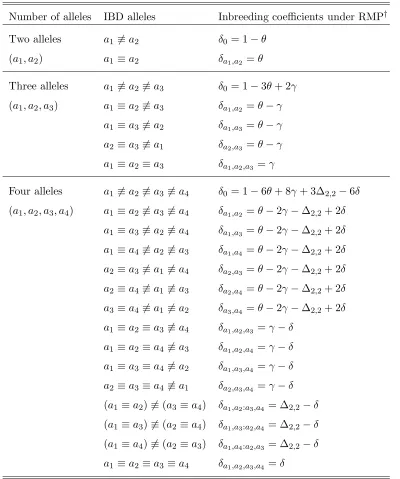
Table 1.2: Inbreeding coefficients for two, three and four alleles and their relation with descent measures under a random mating population

Number of alleles IBD alleles Inbreeding coefficients under RMP† Two alleles a16≡a2 δ0 = 1−θ

(a1, a2) a1≡a2 δa1,a2 =θ

Three alleles a_16≡a_{2 6≡}a₃ δ₀ = 1₋3θ+ 2γ

(a₁, a₂, a₃) a_1≡a_{2 6≡}a₃ δa1,a2 =θ−γ

a_1≡a_{3 6≡}a₂ δa1,a3 =θ−γ

a2≡a3 6≡a1 δa2,a3 =θ−γ

a1≡a2 ≡a3 δa1,a2,a3 =γ

Four alleles a16≡a2 6≡a36≡a4 δ0 = 1−6θ+ 8γ+ 3∆2,2−6δ

(a1, a2, a3, a4) a1≡a2 6≡a36≡a4 δa1,a2 =θ−2γ−∆2,2+ 2δ

a_1≡a_{3 6≡}a_26≡a₄ δa1,a3 =θ−2γ−∆2,2+ 2δ

a_1≡a_{4 6≡}a_26≡a₃ δa1,a4 =θ−2γ−∆2,2+ 2δ

a2≡a3 6≡a16≡a4 δa2,a3 =θ−2γ−∆2,2+ 2δ

a2≡a4 6≡a16≡a3 δa2,a4 =θ−2γ−∆2,2+ 2δ

a3≡a4 6≡a16≡a2 δa3,a4 =θ−2γ−∆2,2+ 2δ

a1≡a2 ≡a36≡a4 δa1,a2,a3 =γ−δ

a_1≡a_{2 ≡}a_46≡a₃ δa1,a2,a4 =γ−δ

a_1≡a_{3 ≡}a_46≡a₂ δa1,a3,a4 =γ−δ

a_2≡a_{3 ≡}a_46≡a₁ δa2,a3,a4 =γ−δ

(a1 ≡a2)6≡(a3≡a4) δa1,a2:a3,a4 = ∆2,2−δ

(a1 ≡a3)6≡(a2≡a4) δa1,a3:a2,a4 = ∆2,2−δ

(a1 ≡a4)6≡(a2≡a3) δa1,a4:a2,a3 = ∆2,2−δ

a1≡a2 ≡a3≡a4 δa1,a2,a3,a4 =δ

1.4

Heterozygosity

Heterozygosity is simply the proportion of individuals with a heterozygous genotype in a population at a single locus. Heterozygosity is often termed observed heterozygosity or Ho. If we have more than one locus then we take the average of observed heterozy-gosity over loci. For the case of species with some degree of selfing, heterozyheterozy-gosity can be inadequate to describe the amount of genetic variation in a population. In this case, it is very common that many different types of homozygous genotypes are present in the population and would not be captured by the frequency of heterozygote. To solve this problem, Nei (1973) proposed another method of gene diversity that captures the diversity at the allelic level. If there are s alleles in a particular locus with frequencies

p1, p2,· · ·ps, then the gene diversity for this locus is defined as 1−Psi=1p2i. If there

is more than one locus, then we take the average of gene diversity over locus. As a measure of genetic variation, Nei’s gene diversity should be particularly used for selfing species. The expected value of observed heterozygosity and the value of gene diversity are the same in a random mating population not undergoing selfing. For this reason, gene diversity has been frequently and incorrectly termed average heterozygosity, or

He in the literature. The relationship between gene diversity and heterozygosity and the coancestry coefficient θcan be expressed exactly for certain specific population and mutation models but may more complicated in real life.

1.5

Wright-Fisher Model

The Wright-Fisher model assumes that the alleles in the current generation are derived by sampling with replacement from the previous generation. In this research we always assume that all the loci that we are interested in are neutral. This means all alleles in a particular locus are equally likely to survive and be transmitted to the next generation. There may be any number of allelic types at a particular locus. Basically given the allele frequencies of the previous generation at reproduction the allele counts in the present generation follow a Multinomial distribution. The index of the distribution is 2N (N is the size of the present population) and the probability vector is the allele frequencies of the previous generation at reproduction. If we have only two allelic types, then the allele counts follow a Binomial distribution with appropriate parameters.

1.6

Theoretical Values of Descent Measures

In this section we discuss how the descent measures change over generations in a random mating population. We consider the Wright-Fisher model for transmitting alleles over generations. The value of the descent measures in a generation depends on the assumption of mutation of alleles, the value of the descent measures in the previous generation and the size of the previous generation. The descent measures at a particular locus do not depend on the number of alleles and allele frequencies in the locus. We denote the value assumed by θ, γ, δ, ∆2,2 at generation t by θt, γt, δt and ∆2,2,t. We assume that there are N individuals i.e. 2N alleles in the population

at time t. We derive expressions for θt+1, γt+1, δt+1 and ∆2,2,t+1. These values can be expressed in terms of N, θt, γt, δt and ∆2,2,t. But we get different expressions for

different assumptions about mutations. In the next two sections we find expressions for the descent measures under different assumptions about mutations.

1.6.1

No Mutation

In this section we assume no mutation among alleles and discuss the behavior of the descent measures. Take two alleles from the population at time t + 1. These two alleles can be descended from one allele or two different alleles at generation t with probabilities ₂1_N and 1_{− 2}1_N respectively. If these two alleles are descended from a single allele then they are always ibd. If the alleles are descended from two different alleles then the probability that they are ibd is θt. So we have

θt+1 = 1

2N + (1−

1

2N)θt. (1.7)

Now we consider three different alleles from (t + 1)th _{generation. We will find the}

probability that these alleles are identical by descent which is denoted by γt+1. These three alleles can be descended from one, two, and three different alleles in the previous generation with probabilities _4N12,

3(2N−1) 4N2 and

(2N−1)(2N−2)

are always ibd if they come from the same allele in the previous generation. If they are descended from two different alleles in the previous generation then the probability that these three alleles are ibd is the same as the probability that the two alleles in the previous generation are ibd which is θt. Similarly if the alleles are descended from three different alleles then the alleles at (t+ 1)th _{generation are ibd with probability} γt. So we get

γt+1 = 1 4N2 +

3(2N ₋1) 4N2 θt+

(2N₋1)(2N ₋2)

4N2 γt. (1.8)

For four alleles, similar arguments as above lead us to the equations

δt+1 = 1 8N3 +

7(2N ₋1) 8N3 θt+

6(2N₋1)(2N ₋2)

8N3 γt

+(2N −1)(2N −2)(2N −3)

8N3 δt and (1.9)

∆2,2,t+1 = 2N

8N3 +

2(4N2₋₁₎ 8N3 θt+

4(2N₋1)(2N ₋2)

8N3 γt

+(2N −1)(2N −2)(2N −3)

8N3 ∆2,2,t. (1.10)

The transition equations (1.7)-(1.10) had been derived by Weir (1994). If the initial population consists of non-inbred and unrelated individuals, then the four descent measures have explicit solutions (Weir, 1994)

θt = 1₋λt₁,

γt = 1₋ 3

2λ t 1+ 1 2λ t 2,

δt = 1₋ 1

5(9λ

t

1−5λt2+λt3)−

3 20(5N ₋3)λ

t

1

+ 1

12(N ₋1)λ

t

2+

8N ₋3

30(5N ₋3)(N ₋1)λ

t

3, and (1.11)

∆2,2,t = 1−

1 15(24λ

t

1−10λ

t

2+λ

t

3)− 1

5(5N ₋3)(λ

t

1−λ

t

where,

λ1 = 1−

1 2N,

λ2 = (1−

1 2N)(1−

2

2N), and (1.12)

λ3 = (1−

1 2N)(1−

2 2N)(1−

3 2N).

The above solutions assume that the population size remains the same over generations and equal to N. If the population size changes over generations and the effective pop-ulation size is Ne, then the above equations approximately hold good if N is replaced by Ne.

Now we approximate the expressions in the equation (1.11) by assuming N _{→ ∞}. We also re-scale the time by assuming a unit time is equal to 2N. In other words we are assuming tis of the order O(N). For notational benefit we denotec= limN→∞ ₂t_N. So for large N and large t we get

λt

1 = exp (−c), λt2 = exp (−3c), and λt3 = exp (−6c). (1.13) WhenN is large, using the above approximation we get the relations (Robertson, 1952)

γ = 3

2θ 2

− 1₂θ3, (1.14)

δ = 3θ3₋3θ4+ 6 5θ

5

− 1₅θ6, and (1.15)

∆2,2 = θ2+ 2 3θ

3_−θ4₊ 2 5θ

5₋ 1 15θ

6 ₌ 2 3γ+

1

3δ. (1.16)

measures become functions of θ and they can be expressed as (Weir, 1994)

γn = 0, δn= 0, and ∆2,2,n=θ2. (1.17)

1.6.2

Both-Way Mutation

In this section we allow both way mutation. We assume any allele mutates to another allele with a positive rate u. Using the same arguments that we have used in the previous section get the following transition equations

θt+1 = (1−u)2[ 1

2N + (1−

1 2N)θt], γt+1 = (1−u)3[

1 4N2 +

3(2N ₋1) 4N2 θt+

(2N ₋1)(2N ₋2) 4N2 γt],

δt+1 = (1−u)4[ 1 8N3 +

7(2N ₋1) 8N3 θt+

6(2N ₋1)(2N ₋2)

8N3 γt

+(2N−1)(2N −2)(2N −3)

8N3 δt], and (1.18)

∆2,2,t+1 = (1−u)4[ 2N

8N3 +

2(4N2₋₁₎ 8N3 θt+

4(2N ₋1)(2N ₋2)

8N3 γt

+(2N−1)(2N −2)(2N −3)

8N3 ∆2,2,t].

The mutation rateuis generally very small. It is safe to assume that the higher orders of u (u2_{, u}3 _{etc) are negligible. Now we assume population sizes are also very large} which says u/N, u/N2_{, u/N}3_{, and 1/N}2 _{are very close to 0. So we can omit them} while doing the algebra. This approximation leads to

θt+1 = 1

2N + (1−2u−

1 2N)θt, γt+1 =

3

2Nθt+ (1−3u−

3 2N)γt, δt+1 =

6

2Nγt+ (1−4u−

6

2N)δt, and (1.19)

∆2,2,t+1 = 2 2Nθt+

4

2Nγt+ (1−4u−

6

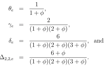
Let us define a new parameter φ = 4Nu. Then at equilibrium the descent measures will be

θe = 1

1 +φ,

γe = 2

(1 +φ)(2 +φ),

δe = 6

(1 +φ)(2 +φ)(3 +φ), and (1.20) ∆2,2,e =

6 +φ

(1 +φ)(2 +φ)(3 +φ).

From the above set of equations we get another set of relations between descent mea-sures for large population size and generation (Balding and Nichols, 1995)

γe = 2θ

2

e

1 +θe,

δe = 6θ

3

e

(1 +θe)(1 + 2θe), and (1.21)

∆2,2,e =

θ2

e(1 + 5θe)

(1 +θe)(1 + 2θe).

true values ofγ andδ that can be calculated using transition equations. The difference is smaller in the both-way mutation model but still there is a significant difference. So we conclude that in general we can not use the normal distribution to approximate γ

0.0 0.5 1.0 1.5 2.0

0.0

0.1

0.2

0.3

0.4

Pure drift model

Time/N

gamma

0.0 0.5 1.0 1.5 2.0

0.000

0.005

0.010

0.015

Infinite allele mutation model

Time/N

gamma

0.0 0.5 1.0 1.5 2.0

0.0

0.1

0.2

0.3

0.4

Time/N

delta

0.0 0.5 1.0 1.5 2.0

0.0000

0.0015

0.0030

Time/N

delta

0.0 0.5 1.0 1.5 2.0

0.0

0.1

0.2

0.3

0.4

Time/N

Delta_{2,2}

0.0 0.5 1.0 1.5 2.0

0.000

0.004

0.008

Time/N

Delta_{2,2}

Figure 1.1: γe, δe, ∆e from equations (1.21) (dotted line) and γn, δn, ∆2,2,n from

Chapter 2

Estimation of Decent Measures

2.1

Introduction

Population structure is a great interest in Genetics. We can make inferences about the history of a population if we know the population structure. The population structure is generally modeled as association between alleles and can be characterized by descent measures. We can also make inferences about the relatedness between two arbitrary individuals in a population using descent measures. There are two types of second order descent measures, total inbreeding (F) and coancestry coefficient (θ). For a random mating population these two parameters are the same. The coancestry coefficient measures the degree of relationship between the individuals within the sub-populations relative to the amount of relationship found in the total population. Higher-order descent measures are useful in special situations. In general, kth_{-order (k ≥2) descent}

frequently used to calculate different expressions in DNA profile matching (Weir, 1994). These descent measures are also useful in affected-relative tests.

The estimation of the descent measureθ and analog ofθhave been discussed widely in the literature (Nei, 1973; Weir and Cockerham, 1984; Robertson and Hill, 1984; Slatkin, 1995). To estimate θ, the frequentist approaches, method of moments and maximum likelihood, and Bayesian methods have been used. The frequentist methods are computationally less intensive while the Bayesian approaches have the benefit of systematic incorporation of prior information about the data which increases the ability to capture important information about parameters in complex cases.

Weir and Cockerham (1984) first obtained the moment estimator ofθ and Robert-son and Hill (1984) followed their method. These two estimators are known as bivariate estimators. Later a multivariate estimator of θ was proposed by Long (1986). The bi-variate estimators are constructed through combining individual alleles linearly over all alleles and loci, while the multivariate estimator is combined only over loci. Long’s esti-mator is equivalent to the Robertson-Hill and Weir-Cockerham estiesti-mators for bi-allelic data from a single locus. Yang (1998) generalized Weir and Cockerham’s estimator to an arbitrary number of levels in a population hierarchy. The above methods do not account for the linkage disequilibrium between loci in combining the information over loci. The best possible way to combine the bivariate estimators over alleles has remained an issue. Weir and Cockerham (1984) combined the estimates by taking the ratio of the sum of the numerators of each estimator to the sum of the denominators of each estimator. Alternatively, Robertson and Hill (1984) combined the estimates by taking weighted average of the ratio estimators over all alleles. Different weights have been proposed for multiple alleles and loci by minimizing the variance of the estima-tor for different ranges of the true value of θ. When the true value of θ is high then the variance of the estimator minimized for the Weir and Cockerham estimator while the Robertson and Hill approach minimized the variance for low to medium value of

Applying Bayesian methods to the problem of inferring population structure has increased in last few years due to affordable computing power. By using the knowledge about populations gained in the past, the robustness of estimates from extreme data sets sampled from the present can be increased (Lange, 1995). The Bayesian methods also make simultaneous inferences about other parameters of interest such as model fit, number of distinct populations in a group of populations etc. The sensitivity and performance of Bayesian estimates depend on the choice of prior. Bayesian approaches to estimation of θ involve the assumption of hierarchial models including the forms of prior parameter and likelihood distributions. The Dirichlet (Balding and Nichols, 1995; Lange, 1995; Holsinger, 1999) and the multivariate normal (Weir and Hill, 2002) are two commonly used forms for the distribution of population allele frequencies with multiple alleles at a locus. For bi-allelic data such as SNP loci, the bivariate forms of these distributions reduce to a Beta and a normal distribution (Smouse and Willams, 1982; Holsinger, 1999; Balding, 2003; Nicholson and Donnelly, 2002). In Bayesian approaches the estimates of θ are the posterior mean of the conditional distribution of the parameters generated by using MCMC based rejection sampling.

The distributions of allele frequencies vary with population models and the time since divergence of populations. The stationary distribution of allele frequencies for most of the stochastic process models, such as, island model (Wright, 1931) and finite stepping-stone model (Maruyama, 1977) is Beta. The normal distribution has been justified by the appeal to large sample theory (Weir and Hill, 2002; Nicholson and Donnelly, 2002) rather than stationary distribution. The normal distribution has been used for non-equilibrium population which are likely to have shorter time since diver-gence (Nicholson and Donnelly, 2002) while a Beta or a Dirichlet distribution is a poor fit. For populations with weak drift and migration, the Dirichlet distribution may be a poor fit for stationary distribution because this increases the time to reach equilibrium. A Dirichlet distribution does also not fit in the population with high stepwise mutation rates (Graham et al., 2000).

structure introduced by simplifying assumption of a common value of θ across all populations. Their results showed that overall estimates of θ from global human data sets were meaningless and the estimates failed to describe the important local patterns and amount of genetic variance. Balding (Balding, 2003) also pointed out that the usual demographic variation and different population sizes in a collection of populations make the value of θ population specific.

Several estimators have now relaxed the constraint that the value ofθ is the same across populations. Weir and Hill (2002) proposed a new parametrization of popula-tion model that defined a parameter specific to each populapopula-tion. This allows different amount of coancestry for different population. The first estimator obtained through a method of moments approach which is a direct extension of the previous Weir and Cockerham (1984) moment estimator of θ. This estimator is a ratio of unbiased esti-mates and therefore expected to be unbiased but it has large sample variance. This method does not assume any form for the distributions of allele frequencies. The second estimator of population-specific θ described by Weir and Hill (2002) was a maximum likelihood estimator. This estimator was developed under the assumption that the sam-ple allele frequencies are multivariate normally distributed. This estimator has several desirable properties, such as invariance to transformation. However, this likelihood estimator is highly unstable when the likelihood function is flat.

In contrast to the frequentist approaches Nicholson and Donnelly (2002) approached this expanded parametrization from a Bayesian point of view, in the context of an application to SNP data. They assumed that the allele frequencies are normally dis-tributed. The authors justify this model as having a reasonable fit to recently diverged, non-equilibrium populations. Balding (2003) also worked with a Bayesian approach but he assumed a Beta distribution for the allele frequency. Holsinger and Wallace (2004) extended Balding’s model for the hierarchical model by describing a summary statistic that compared the posterior and prior distribution of the coancestry parameters.

estimator is yet to be evaluated. If we assume a Dirichlet or a normal distribution for the allele frequencies thenγ becomes a function ofθ. In this case we can infer γ based on the estimate of θ. Unfortunately, these distributions are not realistic for natural populations, such as human populations. So the parameter γ has to be estimated independently. The demographic and size variation in a set of populations make the descent measures population specific. So the value ofγvaries over different population. There is no estimator for a population-specific γ. There are two fourth order descent measures. We will show that these two parameters can not be estimated separately.

In this chapter we propose different estimators of descent measures. First we as-sume the same value of descent measures across the populations and propose a set of moment estimators of θ andγ based on the third order Analysis of Variance statistics. Then we propose another set of estimators of θand γ using a direct probabilistic inter-pretation. We also compare method of moments estimator with probabilistic estimator analytically. Later we assume a population-specific value of descent measures and ex-tend our estimators. To have a better idea about the estimates we also calculate the sampling properties of the estimators. We give the expressions for biases and variances of different estimators. Our estimators have large variances but these variances can be reduced by gathering more information from independent loci.

2.2

Replication of Evolution

be different. The averages can be taken over all possible outcomes of the evolutionary process to get the final value of the parameters. For example, the value of F (or θ) is averaged over sub-populations, and therefore requires an evolutionary model that pre-dicts the levels of variation among sub-populations. Similarly, the value of higher order descent measures γ, δ and ∆2,2, are also averaged over sub-populations. So estimat-ing these parameters require observations from more than one sub-population in order to quantify the variation between sub-populations. These parameters give informa-tion about long-term effects of demographic and evoluinforma-tionary forces of the populainforma-tion. Our expectations will always be over different replications of the populations and any parameter value will be the average value over sub-populations.

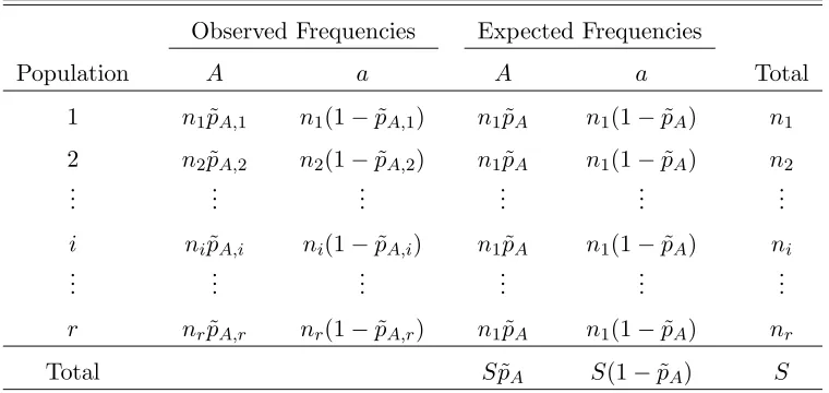
2.3

Data

We have data from the r independent present-day populations. These populations have evolved from a common ancestral population. We will work with locus A. We assume that there are s different allelic forms in locus A namely, A1, A2,· · · , As. The expected allele frequencies in each population are the same and they are p1, p2,· · · , ps respectively. We have ni sampled alleles from the ith _{population. So there are total}

Pr

i=1ni = S sampled alleles. Define a set of indicator functions that describe our frequency data at locus A as follows:

xij,k =     

1 if the jth _{allele ini}th _{population at locus A isAk}

0 otherwise

The observed frequency of the allele Ak in the ith _{population is}

˜

pi,k = 1

ni ni

X

j=1

and the overall weighted and un-weighted observed frequency of the allele Ak are

˜

pw,k = 1

S r

X

i=1

nipi,k˜ and puw,k˜ = 1

r r

X

i=1 ˜

pi,k. (2.2)

When the sample sizes are equal i.e. n1 =n2 =· · ·=nr, then ˜pw,k = ˜puw,k.

2.4

Review of Existing Estimators of

θ

2.4.1

Method of Moments Estimator

A moment estimator ofθwas first found by Weir and Cockerham (1984). They assumed the same value ofθ across different populations. In this section we describe the method of moments (MOM) estimator of θ proposed by Weir and Cockerham (1984). They defined the two mean square statistics based on the frequency of the allele Ak. The mean square statistics are

MSPk = 1

r₋1

r

X

i=1

ni(˜pi,k₋pw,k˜ )2 and (2.3)

MSGk = Pr 1

i=1(ni−1)

r

X

i=1

nipi,k˜ (1₋pi,k˜ ). (2.4)

The expectation of the statistics can be found using the theory

E(xij,kxi′_j′_,k) =     

p2

k+pk(1−pk)θ if i =i′, j 6=j′ p2

k if i6=i′.

(2.5)

The expectations of the mean square statistics are

E(MSPk) = pk(1₋pk)[1 + (nc1 −1)θ] and (2.6)

where

nc1 =

1

r₋1(

r

X

i=1

ni₋

Pr i=1n2i

Pr i=1ni

) = 1

r₋1(S− Pr

i=1n2i

S ).

Using (2.6) and (2.7), Weir and Cockerham (1984) led to their moment estimator of θ,

ˆ

θW C,k = MSPk−MSGk

MSPk+ (nc1 −1)MSGk

. (2.8)

The above estimator is based on the frequency data for the allele Ak. There are different estimators corresponding to different alleles at different loci. After combining information over alleles and loci, Weir and Cockerham (1984) proposed the overall estimator of θ,

ˆ

θW C =

PL l=1

Psl

k=1(MSPlk−MSGlk) PL

l=1 Psl

k=1(MSPl,k+ (nc1 −1)MSGlk)

. (2.9)

whereMSPlk andMSGlk are the two mean square statistics for thekth_{allele at thel}th

locus. They assumed that there are L independent loci and thelth _{locus hassl alleles.}

2.4.2

ML Estimator Based on Normal Distribution

Weir and Hill (2002) proposed an estimator of θ assuming a multivariate normal distribution for allele frequencies. They justified the assumption of normal distribution using large sample sizes and central limit theorem. The normal distribution is an approximate distribution and it works well for small values of θ. Here the authors assumed that ni _{→ ∞} which is equivalent to assume ni =n and n _{→ ∞}. There are s

alleles at locus A which give s₋1 independent allele frequencies. Define a new vector of observed allele frequencies as ˜pi = (˜pi,1,pi,˜ 2,· · · ,pi,s˜ −1)′ ∀i = 1,2,· · ·, r. ˜pi’s are

independent and identically distributed. Weir and Hill (2002) assumed

˜

where p=           p1 p2 ... ps−1          

, C =φ

         

p1(1−p1) −p1p2 . . . −p1ps−1

−p1p2 p2(1−p2) . . . −p2ps−1

... ... _{· · ·} ...

p1ps−1 −p2ps−1 . . . ps−1(1−ps−1)           ,

where φ= _n1[1 + (n₋1)θ]. From standard theory (see Chapter 3), the quadratic form

Q = 1

φ r X i=1 s X k=1

(˜pi,k₋pw,k˜ )2 ˜

pw,k ∼χ

2

(r−1)(s−1). (2.11)

The equation (2.11) gives the maximum likelihood estimate of θ as

ˆ

θN = 1

n₋1

h _n

(r₋1)(s₋1)

r X i=1 s X k=1

(˜pi,k₋pw,k˜ )2 ˜

pw,k −1

i

. (2.12)

If there is more than one loci then the final estimator is the average of the locus specific estimators of θ.

2.4.3

Bayesian Estimator

2.5

New Estimators of

θ

and

γ

2.5.1

Method of Moments Estimator

In this section we propose new moment estimators for θ and γ. We find a set of statistics whose expectations depend on the parameters θ and γ. Then we equate the theoretical moments with sample moments and get the estimators of the parameters. In the expectation of second moment allele frequency, the parameter γ does not appear. This can be seen from the equation (2.5) which does not have γ in its expression. But the parameter γ appears in the expression of third or higher order moments of allele frequencies. The parameterθappears in second or higher order moments of allele frequencies. Here consider two statistics that are based on third order sample moments of allele frequencies. To find the third order moments of the frequency of the alleleAk, we need to use the relation

E(xij,kxi′j′,kxi′′j′′,k) =

          

γpk+ 3(θ₋γ)p2

k+ (1−3θ+ 2γ)p3k if i =i′ = i′′ θp2

k+ (1−θ)p3k if i=i′ 6=i′′ p3

k if i6=i′ 6=i′′.

(2.13)

The above equation (2.13) can also be written as

E(xij,kxi′_j′,kxi′′_j′′_,k) =           

p3

k+ 3p2k(1−pk)θ+pk(1−pk)(1−2pk)γ if i =i′ = i′′ p3

k+p2k(1−pk)θ if i=i′ 6=i′′

p3

k if i6=i′ 6=i′′.

(2.14) The above equation (2.14) shows that when an allele frequency is 0.5, then the third order moment does not depend on γ but it depends on θ. So an allele with frequency 0.5 does not provide any information aboutγ.

moment estimate of θ and γ. The three statistics are

S1,k =

S

(r₋1)(r₋2)

r

X

i=1

ni(˜pi,k₋pw,k˜ )3_,

S2,k =

r

(r₋1)Pr_i=1(ni₋1)

r

X

i=1

n2_ipi,k˜ (1₋pi,k˜ )(˜pi,k₋pw,k˜ ), and (2.15)

S3,k =

1 Pr

i=1(ni−1)(ni−2)

r

X

i=1

n2_ipi,k˜ (1₋pi,k˜ )(1₋2˜pi,k).

Using the equations (2.14) we find the estimate of these three statistics and they are

E(S1,k) =uk(nc2 + 3nc3θ+nc4γ),

E(S2,k) =uk[

r(nc1−1)

S₋r +

r(nc5−4nc1 + 3)

S₋r θ−

r(nc5 −3nc1 + 2)

S₋r γ], and (2.16)

E(S3,k) =uk(1−3θ+ 2γ),

where uk =pk(1₋pk)(1₋2pk) and

nc2 =

1

(r₋1)(r₋2)(S

r

X

i=1 1

ni −3r+ 2),

nc3 =

1

(r₋1)(r₋2)(Sr−S

r

X

i=1 1

ni −3S+ 3r+

2Pr_i=1n2

i

S −2),

nc4 =

1

(r₋1)(r₋2)(S 2

−3Sr+ 2S r

X

i=1 1

ni −3 r

X

i=1

n2i + 9S−6r (2.17)

+2 Pr

i=1n3i

S −

6Pr_i=1n2

i

S + 4), and

nc5 =

1

r₋1(

r

X

i=1

n2i −

Pr i=1n3i

S ).

about the parameters from our statistics. In principle, from the three equations given in the equation (2.16), we can find three statistics T1,k, T2,k and T3,k that are linear

combinations of S1,k,S2,k and S3,k such that

E(T1,k) = pk(1−pk)(1−2pk),

E(T2,k) = pk(1−pk)(1−2pk)θ, and (2.18)

E(T3,k) = pk(1−pk)(1−2pk)γ.

After doing some algebra we get

T1,k = [

2r(nc5 −4nc1 + 3)

S₋r −

3r(nc5 −3nc1 + 2)

S₋r ]S1,k+ (−3nc4 −6nc3)S2,k

+[₋3nc3

r(nc5 −3nc1+ 2)

S₋r −nc4

r(nc5 −4nc1 + 3)

S₋r ]S3,k, T2,k = [−

r(nc5 −3nc1 + 2)

S₋r −

2r(nc1 −1)

S₋r ]S1,k+ (2nc2−nc4)S2,k

+[nc4

r(nc1 −1)

S₋r +nc2

r(nc5 −3nc1 + 2)

S₋r ]S3,k, and (2.19)

T3,k = [−

3r(nc1 −1)

S₋r −

r(nc5−4nc1 + 3)

S₋r ]S1,k+ (3nc3+ 3nc2)S2,k

+[nc2

r(nc5 −4nc1 + 3)

S₋r −3nc3

r(nc1−1)

S₋r ]S3,k.

When T1,k 6= 0 then using ratio estimation theory we get our moment estimator of θ

and γ as

ˆ

θM,k = T2,k

T1,k

I(T1,k 6= 0) and (2.20)

ˆ

γM,k = T3,k

T1,k

I(T1,k 6= 0). (2.21)

different alleles. Here we use both the combining methods to get two sets of estimators. The expectations of the statistics T1,k, T2,k, T3,k are positive when ˜pk < 0.5 and are

negative when ˜pk >0.5. There is only one allele that has frequency greater than 0.5. If we addT1,k over∀k, then there is a chance that we might end up getting some value

very close to 0. For two alleles we always get P2_k=1T1,k = 0. Under these situations

the estimators do not work well if we get the final estimator using Weir-Cockerham’s weight. So we exclude the allele that has observed frequency greater than 0.5 and work with the rest independent allele frequencies. We combine the estimators corresponding to different alleles and different loci by our modified method and get the final estimators

ˆ

θ1,M =

Ps

k=1T2,kI(˜pw,k <0.5) Ps

k=1T1,kI(˜pw,k <0.5)

,

ˆ

θ2,M =

1

s s

X

k=1

T2,k T1,k

I(T1,k 6= 0), (2.22)

ˆ

γ1,M =

Ps

k=1T3,kI(˜pw,k <0.5) Ps

k=1T1,kI(˜pw,k <0.5)

, and

ˆ

γ2,M =

1

s s

X

k=1

T3,k T1,k

I(T1,k 6= 0).

If we have data from Lindependent loci then our final estimators would be

ˆ

θ1,M =

PL l=1T2,l

PL l=1T1,l

, θˆ2,M =

1 L L X l=1 ˆ

θ2,M,l, (2.23)

ˆ

γ1,M =

PL l=1T3,l

PL l=1T1,l

, and γˆ2,M =

1 L L X l=1 ˆ

γ2,M,l, (2.24)

whereθ2,M,land γ2,M,l are the estimators ofθ andγ respectively based on thelth locus. T1,l,T2,l andT3,l are the sum ofT1,k,T2,k andT3,k respectively over different alleles that

equal sample sizes case the equation (2.19) reduces to

T1,k = S1,k+ 3(n−1)S2,k + (n−1)(n−2)S3,k,

T2,k = S1,k+ (n−3)S2,k−(n−2)S3,k, and (2.25)

T3,k = S1,k−3S2,k+ 2S3,k.

2.5.2

Estimators with Probabilistic Interpretation

In this section we provide estimators of θ and γ using a Probabilistic Interpretation. Here we work with the same set up as in the previous sections. If we choose two alleles from a population then the probability that both the alleles are of the type

Ak, depends on the parameter θ. The probability of getting three Ak alleles from a population depends on θ and γ. The above two probabilities depend on the expected frequency of Ak, pk, as well. We explore these probabilities and find estimators of the parameters θ and γ. Now we define a new set of parameters

πi,j,k = Esub−pop[P r(iallele(s) from j population(s) being of the type Ak)]. (2.26)

We are interested in the parameters π1,1,k, π2,1,k, π2,2,k, π3,1,k, π3,2,k and π3,3,k. Using

the population genetics theory we get

π1,1,k = pk, π2,2,k =p2k, π3,3,k =p3k,

π2,1,k = p2k+ (pk−p2k)θ, π3,2,k =p3k+ (pk2 −p3k)θ, and (2.27) π3,1,k = p3k+ 3(p

2

k−p

3

k)θ+ (pk−3p

2

k+ 2p

3

k)γ.

After doing some algebra using the equations in (2.27) we get

θ = π2,1,k−π2,2,k

π1,1,k−π2,2,k

, θ= π3,2,k−π3,3,k

π2,2,k−π3,3,k

and (2.28)

γ = π3,1,k−3π3,2,k + 2π3,3,k

π1,1,k−3π2,2,k + 2π3,3,k

From the equations (2.28) and (2.29), the estimates of the parameters θ and γ based on the kth _{allele frequency at locus A are}

ˆ

θ1,P,k =

ˆ

π2,1,k−πˆ2,2,k

ˆ

π1,1,k−πˆ2,2,k

, θˆ2,P,k =

ˆ

π3,2,k−πˆ3,3,k

ˆ

π2,2,k−πˆ3,3,k

and (2.30)

ˆ

γP,k = πˆ3,1,k−3ˆπ3,2,k+ 2ˆπ3,3,k ˆ

π1,1,k−3ˆπ2,2,k+ 2ˆπ3,3,k

. (2.31)

Now we have to find the estimates of π1,1,k, π2,1,k, π2,2,k, π3,1,k, π3,2,k and π3,3,k. Giving

equal weights to each population, the estimates of the probabilities are

ˆ

π1,1,k =

1 r r X i=1 ˜

pk,i = ˜puw,k,

ˆ

π2,1,k =

1

r r

X

i=1

nip˜2

k,i−pk,i˜ ni₋1 ,

ˆ

π2,2,k =

(Pr_i=1pk,i˜ )2₋Pr i=1p˜2k,i

r(r₋1) , (2.32)

ˆ

π3,1,k =

1 r r X i=1 n2

ip˜3k,i−3nip˜2k,i+ 2˜pk,i

(ni₋1)(ni₋2) ,

ˆ

π3,2,k =

1

r(r₋1) h_Xr

i=1

nip˜2

k,i−pk,i˜ ni₋1

i_Xr

i=1 ˜

pk,i₋ 1

r(r₋1)

r

X

i=1

nip˜3

k,i−p˜2k,i

ni₋1 , and

ˆ

π3,3,k =

(Pr_i=1pk,i˜ )3₋₃₍Pr

i=1pk,i˜ )( Pr

i=1p˜2k,i) + 2(

Pr i=1p˜3k,i)

r(r₋1)(r₋2) .

In theory the equation (2.29) does not exist when pk = 0.5. When pk = 0.5, then the equation provides γ = 0

0 which does not make any sense. This can be observed from the equation (2.14) which says that the third moment of observed frequency of an allele does not involve γ if the allele frequency is 0.5. So whenpk = 0.5, we can not estimate

proposed by Weir and Cockerham (1984) and they combined the estimates by taking the ratio of the sum of the numerators of each estimator to the sum of the denominators of each estimator. Suppose there areLindependent loci and thelth_{locus hasslalleles.}

Then the final estimates based on the Weir-Cockerham’s method are

ˆ

θ1,P =

PL l=1

Psl

k=1(ˆπ2,1,k,l−πˆ2,2,k,l)

PL l=1

Psl

k=1(ˆπ1,1,k,l−πˆ2,2,k,l)

, (2.33)

ˆ

θ2,P =

PL l=1

Psl

k=1(ˆπ3,2,k,l−πˆ3,3,k,l) PL

l=1 Psl

k=1(ˆπ2,2,k,l−πˆ3,3,k,l)

, and (2.34)

ˆ

γ1,P =

PL l=1

Psl

k=1(ˆπ3,1,k,l−3ˆπ3,2,k,l+ 2ˆπ3,3,k,l)I(˜pw,k,l<0.5)

PL l=1

Psl

k=1(ˆπ1,1,k,l−3ˆπ2,2,k,l+ 2ˆπ3,3,k,l)I(˜pw,k,l<0.5)

, (2.35)

where ˆπ1,1,k,l, ˆπ2,1,k,l, ˆπ2,2,k,l, ˆπ3,1,k,l, ˆπ3,2,k,l and ˆπ3,3,k,l are estimate of π1,1,k,π2,1,k,π2,2,k, π3,1,k, π3,2,k and π3,3,k respectively for the lth locus. ˜pw,k,l is the weighted average

frequency of the allele Ak at thelth _locus.

On the other hand, Robertson and Hill (1984) combined the estimates by taking a weighted average of the ratio estimators over all alleles at different locus. Using this method we get another set of estimators

ˆ

θ3,P =

1 L L X l=1 1 sl sl X k=1

(ˆπ2,1,k,l−πˆ2,2,k,l)

(ˆπ1,1,k,l−πˆ2,2,k,l)

, (2.36)

ˆ

θ4,P =

1 L L X l=1 1 sl sl X k=1

(ˆπ3,2,k,l−πˆ3,3,k,l)

(ˆπ2,2,k,l−πˆ3,3,k,l)

, and (2.37)

ˆ

γ2,P =

1 L L X l=1 1 sl sl X k=1

(ˆπ3,1,k,l−3ˆπ3,2,k,l+ 2ˆπ3,3,k,l)

(ˆπ1,1,k,l−3ˆπ2,2,k,l+ 2ˆπ3,3,k,l)

I(denominator₆= 0), (2.38)

where ˆπ1,1,k,l, ˆπ2,1,k,l, ˆπ2,2,k,l, ˆπ3,1,k,l, ˆπ3,2,k,l are ˆπ3,3,k,l are estimates ofπ1,1,k, π2,1,k,π2,2,k, π3,1,k,π3,2,k and π3,3,k respectively for the lth locus.

When sample sizes are equal then ˆθ1,P is exactly the same as θW C, the classical

2.6

New Estimators of Population-specific

θ

and

γ

Long and Kittles (2003) and Balding (2003) showed the overall estimates of descent measures fail to describe the important local patterns and amount of genetic variance because of demographic variances among populations. In this section we assume the value of θ and γ in the ith _{population is θi and γi respectively. Researchers provided}

estimators of θi using different methods such as MOM, ML, and Bayesian methods. In the next section we describe new estimates of the population-specific θ using a probabilistic interpretation. In literature there is no estimator for the population-specific γ. We propose several estimators of the population-specific γ.

2.6.1

Estimators with Probabilistic Interpretation

In this section we provide estimators of population-specificθ andγ using a probabilistic interpretation. For estimating θi and γi we define the following parameters

π2,1,k,i = Esub−pop[P r(Two alleles from ith population are of the type Ak)],

π3,1,k,i = Esub−pop[P r(Three alleles from ith population are of the type Ak)], (2.39) π3,2,k,i = Esub−pop[P r(Two alleles from ith population and one allele from another

population are of the type Ak)].

We also need to consider three more parameters, π1,1,k,π2,2,k andπ3,3,k that are defined

in the equation (2.26). The relation of the above parameters with expected allele frequencies and population-specific descent measures can be found from the equation

E(xij,kxi′j′,kxi′′j′′,k) =

          

p3

k+ 3p2k(1−pk)θi+pk(1−pk)(1−2pk)γi if i = i′ =i′′ p3

k+p2k(1−pk)θi if i=i′ 6=i′′

p3

k if i6=i′ 6=i′′,

and the relations are

π1,1,k = pk, π2,2,k =p2k, π3,3,k =p3k,

π2,1,k,i = p2k+ (pk−p2k)θi, π3,2,k,i=p3k+ (pk2 −p3k)θi, and (2.41) π3,1,k,i = p3k+ 3(p

2

k−p

3

k)θi+ (pk−3p

2

k+ 2p

3

k)γi.

After doing some algebra using the equations in (2.41) we get

θi = π2,1,k,i−π2,2,k

π1,1,k−π2,2,k

, θi = π3,2,k,i−π3,3,k

π2,2,k−π3,3,k

, and (2.42)

γi = π3,1,k,i−3π3,2,k,i+ 2π3,3,k

π1,1,k−3π2,2,k+ 2π3,3,k

. (2.43)

From the equations (2.42) and (2.43), the estimates of the parameters θi and γi based on the frequency data of the allele Ak are

ˆ

θ1,P,k,i =

ˆ

π2,1,k,i−πˆ2,2,k

ˆ

π1,1,k−πˆ2,2,k

, θˆ2,P,k,i=

ˆ

π3,2,k,i−πˆ3,3,k

ˆ

π2,2,k−πˆ3,3,k

, and (2.44)

ˆ

γP,k,i = ˆπ3,1,k,i−3ˆπ3,2,k,i+ 2ˆπ3,3,k ˆ

π1,1,k−3ˆπ2,2,k+ 2ˆπ3,3,k

. (2.45)

Now we have to find the estimates of π1,1,k, π2,1,k,i, π2,2,k, π3,1,k,i, π3,2,k,i and π3,3,k. The

estimates of π1,1,k, π2,2,k and , π3,3,k are given in the equation (2.32). Giving equal

weights to each population, we get the estimates of the other probabilities as

ˆ

π2,1,i,k = nip˜2

k,i−pk,i˜ ni₋1 , ˆ

π3,1,i,k = n2

ip˜3k,i−3nip˜2k,i+ 2˜pk,i

(ni₋1)(ni₋2) , and (2.46)

ˆ

π3,2,i,k =

1 (r₋1)

nip˜2k,i−pk,i˜ ni₋1 (

r

X

j=1 ˜

In theory the equation (2.29) does not exist when pk = 0.5. When pk = 0.5, then the equation provides γi = 0

0 which does not make any sense. So when pk = 0.5, we can not estimate γi from the frequency data of the allele Ak. At this point we have estimators of θi and γi based on a single allele frequency. There are several methods to combine the estimators corresponding different allele frequencies to get a final estimator. Weir and Cockerham (1984) combined the estimates by taking the ratio of the sum of the numerators of each estimator to the sum of the denominators of each estimator. Suppose there are L independent loci and thelth _{locus has sl alleles. Then}

the final estimates based on the Weir-Cockerham’s method are

ˆ

θ1,P,i =

PL l=1

Psl

k=1(ˆπ2,1,k,i,l−πˆ2,2,k,l)

PL l=1

Psl

k=1(ˆπ1,1,k,l−πˆ2,2,k,l)

, (2.47)

ˆ

θ2,P,i =

PL l=1

Psl

k=1(ˆπ3,2,k,i,l−πˆ3,3,k,l)

PL l=1

Psl

k=1(ˆπ2,2,k,l−πˆ3,3,k,l)

, and (2.48)

ˆ

γ1,P,i =

PL l=1

Psl

k=1(ˆπ3,1,k,i,l−3ˆπ3,2,k,i,l+ 2ˆπ3,3,k,l)I(˜pw,k,l<0.5)

PL l=1

Psl

k=1(ˆπ1,1,k,l−3ˆπ2,2,k,l+ 2ˆπ3,3,k,l)I(˜pw,k,l<0.5)

. (2.49)

On the other hand, Robertson and Hill (1984) combined the estimates by taking weighted average of the ratio estimators over all alleles at different locus. Using Robertson-Hill’s method we get another set of estimators

ˆ

θ3,P,i =

1 L L X l=1 1 sl sl X k=1

(ˆπ2,1,k,i,l−πˆ2,2,k,l)

(ˆπ1,1,k,l−πˆ2,2,k,l)

, (2.50)

ˆ

θ4,P,i =

1 L L X l=1 1 sl sl X k=1

(ˆπ3,2,k,i,l−πˆ3,3,k,l)

(ˆπ2,2,k,l−πˆ3,3,k,l)

, and (2.51)

ˆ

γ2,P,i =

1 L L X l=1 1 sl sl X k=1

(ˆπ3,1,k,i,l−3ˆπ3,2,k,i,l+ 2ˆπ3,3,k,l)

(ˆπ1,1,k,l−3ˆπ2,2,k,l+ 2ˆπ3,3,k,l)

I(denominator₆= 0).(2.52)

where ˆπ1,1,k,l, ˆπ2,1,k,i,l, ˆπ2,2,k,l, ˆπ3,1,k,i,l, ˆπ3,2,k,i,land ˆπ3,3,k,lare the estimate ofπ1,1,k,π2,1,i,k, π2,2,k,π3,1,i,k,π3,2,i,kandπ3,3,krespectively for thelthlocus. ˜pw,k,lis the weighted average

2.6.2

Method of Moments Estimator

In this section we propose a new estimator of population-specific γ. The estimator is based on the MOM approach. For estimating γi we propose a new statistic

S3,k,i =

n2

i

(ni₋1)(ni₋2)pi,k˜ (1−pi,k˜ )(1−2˜pi,k), (2.53)

and the expectation of the statistic is

E(S3,k,i) = pk(1−pk)(1−2pk)(1−3θi+ 2γi). (2.54)

Let us assume ˆθW H,i is the moment estimator of θi proposed by Weir and Hill (2002). Since this is a moment estimator, the bias of the estimator is close to zero. So we can assume E(ˆθW H,i)_≈θi. Using ratio estimate we get

Eh

Ps

k=1S3,k,i

1₋3Ps_k=1πˆ2,2,k+ 2

Ps

k=1πˆ3,3,k

+ 1.5ˆθW H,i₋0.5i

≈ E(

Ps

k=1S3,k,i)

2[1₋3E(π2,2) + 2E(π3,3)]

+ E(1.5θW H,i)₋0.5

≈ (1−3

Ps

k=1p2k+ 2

Ps

k=1p3k)(1−3θi+ 2γi)

2(1₋3Ps_k=1p2

k+ 2

Ps k=1p3k)

+ 1.5θi₋0.5 = γi.

So a moment estimator of γi based on locus A is

ˆ

γM,i =

Ps

k=1S3,k,i

1₋3Ps_k=1πˆ2,2,k+ 2

Ps

k=1πˆ3,3,k

+ 1.5ˆθW H,i₋0.5. (2.55)

2.7

Bias and Variance of the Estimators

can find expressions for bias and variance of the estimators which are multi-allelic, and have unequal sample sizes; in practice they are intractable. So we restrict our research to a simple situation. We assume that there are L independent loci and each locus has two different allelic forms. So the estimators of the descent measures are based on one allelic frequency at each locus. Our expressions for bias and variance will be developed based on a locusA and then extended them for a multi-locus situation. The locusA has two alleles,A anda, with expected frequenciespA and 1₋pA respectively. Without loss of generality we work with the frequency of the allele A, pA. We also assume that each population has the same sample size, n. The descent measures have the same value in different populations.

Our estimators are based on the second and third moments of allele frequencies. The bias and variance of an estimator that is based on second order allele frequencies involve second, third, and fourth order descent measures. If the estimator is based on third order allele frequencies then the bias and variance involve second, third, fourth, fifth, and sixth order descent measures. In the literature we have descriptions about second, third, and fourth order descent measures. Here we define fifth and sixth order decent measures. There are two different types of fifth order descent measure and four different sixth order descent measures. We parameterize all these descent measures as:

η = Esub−pop[P r(Five random alleles are ibd)],

∆3,2 = Esub−pop[P r(Three and two random allele are ibd)], τ = Esub−pop[P r(Six random alleles are ibd)],

∆4,2 = Esub−pop[P r(Four and two random alleles are ibd)], (2.56)

∆3,3 = Esub−pop[P r(Two sets of three random alleles are ibd)], and

∆2,2,2 = Esub−pop[P r(Three random pairs of alleles are ibd)].

Let us denote P∗_{(an event) = E}

sub−pop[P r(an event)]. Now suppose we have five/six