ABSTRACT
ARESHKIN, DENIS ALEXEYEVICH. SELF-CONSISTENT ENVIRON-MENT-DEPENDENT TIGHT-BINDING. METHODOLOGY AND APPLICATIONS. (Under direction of Professor Donald W. Brenner)
We developed a hybrid scheme for hydrocarbons based on Density Functional Theory, which is the self-consistent extension of the Environment Dependent Tight Bind-ing (EDTB) method for carbon. The EDTB model refers to an orthogonal minimal basis set tight-binding (TB) method with two-center hopping matrix integrals that depend not only on the mutual arrangement of the two atoms on which the basis functions are cen-tered, but also on the arrangement of neighboring atoms as well. The EDTB model effec-tively includes the dependence of hopping integrals on the surrounding electron density. This feature makes the EDTB approach highly transferable compared to standard TB, and in many cases this method can produce even better results than DFT with the same num-ber of basis functions per atom.
SELF-CONSISTENT ENVIRONMENT-DEPENDENT
TIGHT-BINDING. METHODOLOGY AND APPLICATIONS.
By
ARESHKIN, DENIS ALEXEYEVICH
A dissertation submitted to the Graduate Faculty of North Carolina State University in partial fulfillment of the requirements for the Degree of Doctor of Philosophy
DEPARTMENT OF MATERIALS SCIENCE AND ENGINEERING
BIOGRAPHY
ACKNOWLEDGEMENTS
TABLE OF CONTENTS
Page List of Tables ____________________________________________________ vi List of Figures ____________________________________________________ vii 1. Context _______________________________________________________ 1 2. Self-consistent tight binding model adapted for hydrocarbon systems _____ 4 2.1 Review of self-consistent tight-binding schemes ______________ 4 2.2 Environment-dependent tight-binding _______________________ 7 2.3 Self-consistent tight binding model _________________________ 8 2.4 Example: Properties of nanodiamond clusters related to field emission 25 2.5 Summary _______________________________________________ 35 3. Convergence acceleration scheme for self-consistent orthogonal-basis-set
LIST OF TABLES
Page 2.1 Optimized carbon orbital parameters _______________________________ 17 2.2 Mulliken populations for a C5 linear chain in external electric fields _______ 17
2.3 Dipole moment and energy decrease for a C5 linear chain ______________ 22
LIST OF FIGURES
Page 2.1 DFT and SC-EDTB spectra for cyclic
C6
_________________________ 15
2.2 Properties of a diamond cluster composed of 161 carbon atoms _______ 18 2.3 Methane, ethane, and benzene
spec-tra
____________________________ 19
2.4 Properties of a hydrogen-passivated diamond cluster composed of 34 atoms 24 2.5 Illustration of inhomogeneous emission
mecha-nism
_________________ 27
2.6 Illustration of homogeneous emission through a ND cluster __________ 27 2.7 Eigenvalue spectrum for 5-7 membered ring ta-C
clus-ter
_____________ 28
2.8 Homogeneous emission mechanism simula-tion
____________________ 29
2.9 Inhomogeneous emission mechanism simula-tion
___________________ 31
3.1 Sample semiconductor spectrum partition-ing
______________________ 51
3.2 Sample metallic spectrum partition-ing
____________________________ 54
3.3 Illustration of typical SC-EDTB conver-gence
______________________ 65
3.4 Eigenvalue spectra of a hydrogen passivated nano-diamond cluster in differ-ent applied field strengths ____________________________________ 67 3.5 Coulomb potential profile along the <001> and <111> lines __________ 68 3.6 Electron potential in the vicinity and inside the cluster when 0.2 V/Ǻ field is
applied _____________________________________________________ 69 3.7 Electron potential in the vicinity and inside the cluster when 2.0 V/Ǻ field is
3.8 Coulomb potential along 5x5 open-ended and capped SWNT’s
________ 72
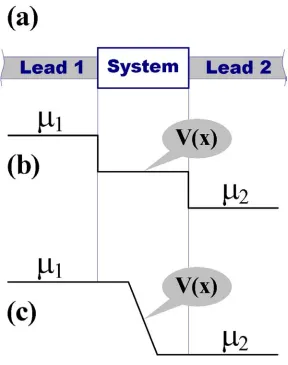
3.9 2D Coulomb potential plots for the open-ended and capped SWNT’s ___ 73 3.10 2D Coulomb potential for a kinked (9,0) SWNT under 0.2 V/Ǻ applied field 75 3.11 Schematic layout considered in many transport
prob-lems
_____________ 76
4.1a SC-EDTB dispersion curves for a (6,0) SWNT ____________________ 82 4.1b SC-EDTB energy density for a (6,0)
SWNT
________________________ 83
4.2 Sample integration contour used to evaluate the density ma-trix
_________ 84
4.3 6-acene molecule ____________________________________________ 93 4.4 SC-EDTB dispersion curves for a polyacene chain _________________ 94 4.5 Test structure used to check the algorithm for electron density evaluation in
open systems under zero applied bias _____________________________ 95 4.6 An example of the open system ________________________________ 95 4.7 An example of an open system with a strong built-in field ____________ 98 4.8 The isolated system used to check the the algorithm for open systems ___ 99 4.9 The sample integration contour used to evaluate the density matrix when
bias is applied between two leads ________________________________ 103 4.10 Polyacene dispersion curves in the vicinity of the Fermi
level
__________ 104
4.11 Approximation of spectral densities ρ9
( )
ε and ρ10( )
ε ______________ 105 4.12 The variable mesh grid used to evaluate and on the realaxis
R
G1,1 GRL
∞
∞, ___ 108
4.13 Evolution of the real axis integration grid with an increase of the applied bias ________________________________________________________ 109 4.14 The set of sampling points used to evaluate non-equilibrium density ____ 112 4.15 Potential distribution for a three-cell polyacene fragment connected to
4.16 The Coulomb potential along the axial line for the system shown in Fig. 4.15 _______________________________________________________ 116 4.17 The layout for the Coulomb potential plots associated with the
non-equilibrium density ___________________________________________ 117 4.18 Coulomb potential distribution for the system composed of two unit cells _ 122 4.19 Coulomb potential distribution for the system composed of four unit cells _ 123 4.20 Coulomb potential distribution for the system composed of six unit cells _ 124 4.21 Coulomb potential distribution for the system composed of eight unit cells 125 4.22 Coulomb potential profile along the axis of the disconnected polyacene
chain; system is composed of six unit cells ________________________ 126 4.23 Coulomb potential profile along the axis of the disconnected polyacene
chain; system is composed of eight unit cells _______________________ 127 4.24 Coulomb potential plots for the system composed of six unit cells
corre-sponding to applied voltages {0.05 V, 0.10 V, 0.15 V …0.95 V, 1.00 V} _ 128 4.25 Coulomb potential plots for the system composed of eight unit cells
corre-sponding to the applied voltages {0.05 V, 0.15 V, 0.25 V …0.85 V, 0.95 V} 128 4.26 The Coulomb potential along the line parallel to the disconnected polyacene
chain for the system composed of six unit cells _____________________ 129 4.27 The Coulomb potential along the line parallel to the disconnected polyacene
chain for the system composed of eight unit cells ____________________ 130 4.28 Coulomb potential plots for the system composed of six unit cells
corre-sponding to the applied voltages {0.05 V, 0.10 V, 0.15 V …0.95 V, 1.00 V} 131 4.29 Coulomb potential plots for the system composed of eight unit cells
corre-sponding to applied voltages {0.05 V, 0.15 V, 0.25 V …0.85 V, 0.95 V} _ 131 4.30 Potential variation along the axis of the system composed of 14 unit cells
when the right lead is biased by 1.0 V _____________________________ 132 4.31 Coulomb potential along the line lying 4.3 Å apart from the axis in the plane
1. CONTEXT
Recently substantial experimental and theoretical49-71 advancements have been made in the field of quantum transport (for a review see Ref. [45] and references therein). The long-term goal of this research is to build high frequency nanoelectronics compo-nents that operate in the THz range. A reliable tool for quantum transport simulation is a key component for nanoelectronics progress. Time-dependent cases require either the Keldysh51,69 or Kadanoff-Baym-Keldysh70 nonequilibrium Green’s function techniques, or alternatively linear response theory and the Kubo formalism.71 As demonstrated by Roland and coworkers51 the response of nanotubes to driving ac voltages with frequen-cies below 0.1 eV ≈ 20 THz is similar to the steady state response. This means that non-equilibrium behavior with f < 10 THz can be safely modeled with steady-state tools. Such a simulation requires only Landauer’s formula68 or a Non-Equilibrium Green’s Function (NEGF) technique44,55 to evaluate current or current density at a given instance of time, plus Poisson’s and continuity equations. Thus, the nearest objective in quantum transport modeling is to apply a NEGF to systems with realistic sizes and within time spans of practical interest.
of object, e.g. a π-electron TB Hamiltonian51,63,64,66 for nanotube simulations. Addition-ally, the non-self-consistent nature of TB does not allow non-equilibrium density simula-tions, which is an essential component of the NEGF technique. Furthermore, self-consistency is needed for simulations of capacitive behavior in time dependent cases.
sources contributing to the current or current density evaluation. Besides the errors in the Hamiltonian matrix, sources of error include errors due to the equilibrium density as-sumption49,50 and the assumption about coupling coefficients49; approximating the spec-tral density for the leads by constants49,59,67; the screening approximation46; and substitut-ing the potential associated with the leads by a linearly changsubstitut-ing potential.55 Our NEGF simulation presented in Section 4 uses none of these assumptions due to the computa-tional efficiency of the SC-EDTB model. Another manifestation of the suitability of the SC-EDTB model for NEGF computation is a real axis integration of van Hove singulari-ties. The small Hamiltonian size allows a sufficient number of sampling points to be produced for integral convergence.
Under nonequilibrium conditions, even at zero temperature, there is finite prob-ability of phonon scattering. As was noted by Hall61 the average time of residency of an electron in a molecule with resistance 12.9 kΩ is 2.1 fs, which is short compared to mo-lecular vibration periods (a fast vibration, such as an OH stretch, has a period of 10 fs). Practical resistances are often three or more orders of magnitude larger than the quantum of resistance and so residence times can become of the order of vibrational periods; hence inelastic scattering events can become important. Inelastic scattering smears the fine spectral structure, which makes a precise evaluation of the Hamiltonian matrix less im-portant for transport problems. The possible degree of smear can be appreciated from the current through a polyacene molecular wire computed by Treboux.60 The current for the first exited state is about 30% higher than the current through the ground state.
2. SELF-CONSISTENT TIGHT BINDING MODEL ADAPTED FOR
HYDROCARBON SYSTEMS
2.1 REVIEW OF SELF-CONSISTENT TIGHT-BINDING SCHEMES
The EDTB model was not the first attempt to include three center integrals in a TB scheme. In 1989 Sankey and Niklewski introduced a parameter free density func-tional (DF) TB scheme that is essentially a minimal non-orthogonal basis set DF calcula-tion, but with matrix elements precalculated on a coarse grid.5 Interpolation between grid points is used to evaluate matrix elements for the given set of distances and angles. Frauenheim and co-workers introduced a similar DF-TB scheme based on two-center in-tegrals.6
The main advantage of the DF-TB schemes over other TB approaches is that in principle they do not require parameter fitting. However, the DF-TB models use a fixed atomic orbital basis, while the EDTB method accommodates the “orbitals” to atomic en-vironments, a potential advantage in terms of the transferability of the scheme for de-scribing electronic states of carbon in different bonding configurations.
To further expand the transferability and functionality of TB schemes, a number of methods have been implemented that introduce self-consistency into TB electronic states (see [1] for a review). Historically, most of these involved modifications to exist-ing non-self-consistent schemes. For example, Frauenheim et al. enhanced a two-center DF-TB approach6 by adding self-consistent (SC) terms7 and spin polarization8 that could be used with an O(N) scaling scheme.9 Similarly, SC versions of Sankey’s multicenter DF-TB scheme,10 as well as Halley and coworker’s TB approach11,12 have been intro-duced, with the latter adding spin-polarized terms to study magnetic systems.13
EDTB matrix H0, and SC corrections ∆H. The latter accounts for charge transfer be-tween constituent atoms, and is supposed to be zero for periodic structures for which the original non-SC EDTB parameterization was made. To be consistent with its initial im-plementation, the EDTB should be extended to include self-consistency by using a DF based approach analogous to Ref. [6,11,14] but for a basis set that is adjustable to differ-ent atomic environmdiffer-ents. However, we approach the problem in a less efficidiffer-ent, though simpler manner and use an environment independent basis to compute ∆H.
The atomic basis functions were chosen by fitting to fully first principles molecu-lar spectra and charge distributions. To satisfy an orthogonality requirement imposed by a convergence acceleration scheme that is used in conjunction with the SC-EDTB method,15 and to be consistent with the original EDTB, orthogonality of atomic orbitals is assumed when evaluating the Hartree and exchange integrals required for ∆H. All Har-tree integrals are otherwise evaluated exactly. Exchange integrals are evaluated ap-proximately as a first-order expansion over an equilibrium electron density. The correla-tion potential and hence correlacorrela-tion integrals are neglected. As shown below, the SC-EDTB scheme is highly transferable compared to standard TB, and in many cases pro-duces better results than minimal orthogonal basis set DF or DF TB.
nano-clusters is due to hydrogen-assisted emission from the edges of small, unpassivated is-lands, consistent with prior models that explain the field emission properties of polycrys-talline diamond. The final section contains some concluding remarks about the SC-EDTB scheme, including comments regarding the applicability of this method for model-ing non-equilibrium electron transport in carbon nanostructures.
2.2 ENVIRONMENT DEPENDENT TIGHT BINDING SCHEME
The traditional feature of most TB methods is a two center Hamiltonian matrix parameterization, which implies the neglect of three and four center integrals as well as nonlinearities of the exchange-correlation potential.1 This means that the contribution of the molecular potential V(r) to the Hamiltonian matrix element Hαβ is restricted to
<ϕα|Vi(r)|ϕβ> where either atomic orbital ϕα or ϕβ belongs to ith atom producing
poten-tial Vi(r). To augment the contributions with index i belonging to atomic sites other than
those on which ϕα or ϕβ are centered, the original EDTB uses a screening function Sαβ
and a scaling function Rαβ that transform the conventional form for two center
Hamilto-nian matrix elements as Hαβ(rαβ) → Hαβ[Rαβ(rαβ)](1- Sαβ). The parameterized functions
Sαβ and Rαβ depend on positions of neighbor atoms, and are designed to account for the
influence of atomic environment on two-center Hamiltonian matrix elements. For exam-ple, when no other atoms are in the vicinity of the line connecting ϕα or ϕβ, Sαβ is zero.
When an extra atom appears between ϕα and ϕβ the value of Sαβ increases because the
The function Rαβ has four parameters, and Sαβ uses separate sets of four
parame-ters for each type of hopping integral, allowing a good fit to band structures from DF cal-culations for six lattice types with atomic coordinations that vary from 2 to 12. The vari-ety of fitted band structures helps to ensure that the EDTB method is applicable to non-periodic systems and is more transferable compared to conventional TB. For example, an indirect bandgap for diamond vs. a direct band gap given by the Xu et al. parameteriza-tion2is achieved with the EDTB method.
2.3 SC-EDTB METHOD
The present section describes modifications made to the EDTB scheme to account for SC charge transfer, and the additional parameterization of matrix elements for C-H bonds. TB may be thought of as a simplified DF scheme for which Hamiltonian elements rather than basis functions are specified. A major simplification of non-SC TB is the as-sumption of electro-neutrality for each constituent atom. To take charge transfer into ac-count in our SC implementation, a basis set must initially be assumed. After atomic orbi-tals ϕζ(r) are chosen, the output electron density ρout(r) is evaluated in a standard manner by using the aufbau principle:
( )
( ) ( )
{ }
ρ ϕα ϕβ α
α β α β
out r r r f Ci Cii
i N N
=
= = =
∈
∑
∑
1SameAtom, 1 1 ,
β
[ ]
fi ≡ f εi =
[
1+exp(
ε µi−)
]
−1kT .
Here is the component of ith eigenvector of the Hamiltonian matrix H = H(ρin) ≡ H0 + ∆H(ρin), ρin is the input electron density from a previous SC iteration, and
Ciζ ζth
εi is the ith Hamiltonian eigenvalue. Because orbital orthogonality is assumed, Eq.(2.1a) contains only the products with indexes α and β belonging to the same atom.
Instead of electron densities, uncompensated Mulliken populations (MP)
qαβ =2
∑
iN=1/2Ci Ciα β −q0α αβδif T = 0 (2.1b)
qαβ =2
∑
iN=1f Ci Cii α β −q0α αβδ if T > 0 (2.1c) are used below. Here δαβ is the Kronneker delta, and is the orbital MP in the bulk material for which the EDTB parameterization has been performed. The additional Cou-lomb potential due to the uncompensated charge isq0α
( )
( ) ( )
{ }
U r q R R
r R dR
N = −
∫
∑
= = ∈ αβ α β α β α β ϕ ϕ1, 1 , SameAtom
. (2.2)
U(r) is termed the additional Coulomb potential because it is produced by the electron density which is the addition to the reference density from the original EDTB parameteri-zation. If a minimal basis set is used, i.e. four orbitals per carbon and one per hydrogen atom, the reference density for a hydrocarbon system is defined as
( )
( )
( )
[
( )
( )
( )
]
{
}
ρ ϕ
ϕ ϕ ϕ ϕ
ref H i
i
s s i p px i py i pz i
i
r r
q0 r q0 r r r
= + + + + ∈ ∈
∑
∑
22 2 2
where ϕH, ϕs, and ϕpx py pz, , Ri
are hydrogen s, and carbon s and p orbitals, respectively, and where is the ith atom position. The original EDTB parametrization was chosen to fit DF band structures for linear, graphite, diamond, simple-cubic (sc), body-centered cubic (bcc), and face-centered cubic (fcc) carbon lattices. In diamond, sc, bcc, and fcc lattices the orbital MP’s are evenly distributed between the x, y, and z p-orbitals. However, the partitioning of the MP’s between s and p-orbitals are unique for each lattice type. For example, for the diamond lattice MP’s obtained using the original EDTB are 1.20285 and
ri = r− i
q0s R
= q0p = 0.93238, while this partitioning is reverted to and for the sc lattice. Hamiltonian matrix elements for periodic lattices do not need any additional corrections related to local charge transfer. These are ac-counted for by the EDTB parameters. The additional potential, as given by Eq.(2.2), should be zero for every periodic lattice used in the EDTB parameterization. This re-quirement obviously cannot be satisfied if the basis functions
q0s <1 q0p >1
ϕs and ϕpx py pz, ,
p
have dif-ferent radial components, and and q0 are assumed to be constants independent of atomic environment. For the sake of simplicity constant and values are used that are equal to MP’s in diamond. Fortunately, this simplification does not have strong effect on the Hamiltonian. Of the periodic structures used to parameterize the EDTB model for carbon, the linear chain gives the largest magnitude of additional Coulomb po-tential. Within a small region near the nucleus it achieves a value of ~0.7 V, which re-sults in non-physical spectrum line shifts of less than 0.45 eV. Other periodic lattices have smaller deviations from the reference density (2.3), and hence smaller non-physical additions to the Hamiltonian matrix elements. If a moment decomposition is used for the
q0s p
difference between the electron densities of sp and sp3 hybridized atoms, the lowest-order nonzero moment is a quadrupole. The resulting short-ranged additional Coulomb potential decays as R-3. Therefore it does not have much effect on the overall system spectrum and charge distribution.
After the reference density ρref has been chosen it becomes possible to use a first
order expansion for the exchange potential Vex
( )
ρ = −ρ1 3 3 1 3( )
π( )
[ ]
[
( )
]
Vex ρ r =Vex ρref r + ∆Vex
where
( )
[
( )
( )
]
( )
( ) ( )
{ }∆V V r r
q V r r r
ex ex ref
ex ref ref ≈ = − = = = ∈
∑
∂ ρ ρ ρ ∂ ϕ ρ ρ ρ αβ ρ ρ ρ α β α β α β .1, 1 , SameAtom
=
ϕ (2.4)
Expansion (2.4) together with Eq.(2.2) is a key condition for establishing a linear rela-tionship between the input and output MP’s that can be utilized, for example, by a New-ton-Raphson convergence technique. The overall SC correction ∆Hαβ to an EDTB ma-trix element with indices α and β belonging to the same atom is
{ }
( ) ( ) ( ) ( )
( ) ( ) ( ) ( )
( )
{ }
∆H q r r R R
r R dRdr
q r r r r V
N ex ref αβ γδ γ δ γ δ α β γ δ γδ α β γ δ ρ ρ ρ γ δ α β γ δ ϕ ϕ ϕ ϕ ϕ ϕ ϕ ϕ ∂ ρ = − + = = ∈ = ∈
∑
∫
∫
∫
∑
1, 1 , , , , , SameAtom SameAtom . dr (2.5)
common way to approximate ∆Hαβ when α and β account for the atomic orbitals situ-ated on different atoms is
( )
(
H 1S
2
ζ
V α
= +V β
α
)
[
]
∆ αβ αβ r r . (2.6)
Here V is a sum of applied and additional Coulomb and exchange potentials, is the position of the atom on which the atomic orbital is centered, and is the overlap matrix element.
rζ
th S
αβ
Because an orthogonal basis set is assumed, Eq.(2.6) is zero. At first, however, it may seem that the quality of a SC-EDTB scheme would benefit if non-zero overlap be-tween neighboring atomic orbitals for Eq.(2.6) is assumed, while keeping S an identity matrix for eigenproblem solving. The following reasoning is used to show that parameterization benefits in the case where S is a unity matrix. Suppose that the entire system has been placed inside a constant potential field V(r) = V0. This shifts the entire eigenvalue spectrum by the amount V0, but in all other ways the spectrum should remain unchanged. Indeed, that is the case if Sαβ is the unity matrix, because all diagonal Hamiltonian elements are increased by V0, while non-diagonal elements remain intact. The assumption Sαβ ≠0 for ≠β in Eq.(2.6) leads to the alteration of some of the non-diagonal Hamiltonian elements, and hence to changes other than a mere shift of the whole spectrum. Therefore the self-consistent correction and the correction due to the applied field are applied only to Hamiltonian elements Hαβ with α and β belonging to the same atom. The correction due to the external electric field with components , , and is
Ex Ey
( ) (
[
)
(
)
(
)
]
( )
∆H
r E x xx E yy y E z zz r dr
αβ
α β
ϕ ϕ
external =
− + − + −
∫
0 0 0 . (2.7)where
(
x y z0, 0, 0)
is the point where the applied potential equals zero.A Gaussian basis set is chosen to allow fast analytical evaluation of the Hartree and exchange integrals. The functional forms for carbon and hydrogen atomic orbitals are given by Eqs. (2.8a) and (2.8b), respectively,
(
)
(
)
(
)
ϕ ϕ
π
α α
s
p
A as r A as
ap X apr
= − + −
=
−
1 1 2 2 2 2
5 4
3 4
2
2 2
exp exp
exp
/ /
r
(2.8a)
(
)
ϕ
π
H =a3 4 −a
3 4
2
2
/ / exp r
(2.8b) where is either x, y or z. The coefficient A2 is obtained from the normalization condition, an A as as2, and p are chosen to provide the best fit to DF spectra and charge distributions of cyclic C6 and a C5 linear chain.16 Because the original EDTB method was developed for pure carbon systems, the parameters , , and used to describe C-H bond and parameter a for the
Xα
d 1, 1, a
EHOnSite SSσ SPσ ϕH atomic orbital must be defined. No interaction between neutrally charged hydrogen atoms is assumed.
value of constant shift to be added to every EDTB spectral line to obtain the best fit to a corresponding DF spectra. A brief comment is needed about the quality of TB spec-tra. The minimal basis set can adequately reproduce low-lying smooth wave functions, and consequently low-lying eigenvalues, but it is insufficient to describe higher energy unoccupied states corresponding to more geometrically involved eigenfunctions. The goal of this parameterization is to obtain electronic properties of the system rather than total energies. For that reason matching both occupied and unoccupied levels is empha-sized, at least in the vicinity of Fermi energy. To optimize the weighed squared differences between the EDTB and DFT spectra for cyclic C6 is minimized. The highest weights were assigned for levels lying near the HOMO and LUMO orbitals, lower weights for other occupied levels, and the lowest weights for high unoccupied levels. The resulting value of is -5.96 eV. Plotted in Fig. 2.1 are DF and SC-EDTB spec-tra for cyclic C6, where the latter is shifted by .
EShift
EShift
EShift
EShift
The next step is to find , , , and coefficients for carbon orbitals. These parameters were obtained by matching C5 linear chain and cyclic C6 MP’s and SC-EDTB spectra lines (shifted by ) to their DFT counterparts. However, an issue inherent to many parameterization problems is encountered. The target function (TF) for parameter optimization usually includes several target subfunctions. For example, when optimizing parameters for carbon orbitals it is desirable to minimize the squared devia-tions for eigenvalues in two different molecules, linear C5 and cyclic C6. Furthermore the TF should include squared MP deviations for cyclic C6, together with squared MP deviations for linear C5 in various applied electric fields. To ensure the correct weights for different target subfunctions accounting for charge and energy, the derivative of
on-A1 as1
Shift
as2 ap
site SC-EDTB Hamiltonian matrix elements is evaluated with respect to the total MP on that site. Although these derivatives may vary substantially depending on a particular atom in a C5 chain, they still provide an idea of how MP deviations should be weighted if one needs to add them to deviations of energy levels:
(
)
[
]
{ }
(
)
TF E E E
EOnSite
MP MP MP
i i
i k
k k
j j
j
= − + +
−
∑
∑
∈
DFT SCEDTB
Shift
all atom sites
DFT SCEDTB 2
2 ∂
∂ .
SCEDTB
(2.9)
Here denotes averaging over all atoms.
FIG. 2.1 DFT (top) and SC-EDTB (bottom) spectra for cyclic C6. The line lengths are
proportional to the degeneracy of the levels; short lines correspond to non-degenerate levels. The C6 ring spectrum as well as all other SC-EDTB spectra shown below are
Frequently the line orders in EDTB and DFT spectra are different. Hence SC-EDTB line order number is an unsuitable argument for choosing its DF counterpart. The analysis of wave function symmetry is the only reliable way to link a SC-EDTB line to its DF analog. Symmetry analysis needs to be performed multiple times because spectra are matched iteratively. The symmetry analysis algorithm becomes too intricate even for molecules like linear C5. A reasonable alternative is spectra moments matching; the sum of squared normalized differences between 20 first spectra moments for linear C5 and cyclic C6 is minimized. The TF also includes linear C5 squared atomic MP deviations for various applied fields. The field is directed along the chain and its magnitude has six different values, 0.0, 0.514, 1.028, 1.542, 2.056, and 2.571 V/Ǻ (Table 2.2). In addition, separate values of MP for s and p-orbitals for cyclic C6 are matched. The values for car-bon orbital parameters are given in Table 2.1. Plotted in Fig. 2.2 are the density of states and potential profile for a diamond cluster composed of 161 atoms. An analytical poten-tial17 is used to relax clusters presented throughout this paper to their minimum energy configuration.
To complete the parametrization, the hydrogen orbital coefficient a (2.8b), and C-H bond parameters , , and together with their scaling function must be defined. The scaling functions for , and are taken from the work by Davidson and Pickett.18 This function reproduces the DF dependence of occupied eigenlevels vs. C-H bond length in methane. At the same time a choice must be made for , , and because these parameters complement the SC corrections. In addition, the values for , , and given by Davidson and Pickett lead to the wrong signs for MP’s for C-H bonds; carbon appears to be less electronegative than hydrogen.
EHOnSite
SSσ
SSσ
SP
SPσ
SSσ
σ
SPσ
EHOnSite
SSσ SPσ
TABLE 2.1 Optimized carbon orbital parameters. , , and are in Ǻ-2. To
con-serve orbital normalization high precision is given for these parameter; however, only the two first significant digits have physical meaning. The parameter choice is not unique as the target function is not unique.
as1 as2 ap
A1 A2 as1 as2 ap
0.08215645 0.5980878 0.1129953 1.500468 1.608523
TABLE 2.2 MP’s for a C5 linear chain in external electric fields of different magnitude.
The SC-EDTB values were obtained with the parameters given in Table 2.1.
Field [V/Ǻ] Method Atom #1 Atom #2 Atom #3 Atom #4 Atom #5 SC-EDTB -0.067 0.231 -0.329 0.231 -0.067 0.000
DFT -0.001 0.095 -0.188 0.095 -0.001 SC-EDTB 0.030 0.235 -0.327 0.224 -0.162 0.514
DFT 0.122 0.129 -0.196 0.055 -0.111
SC-EDTB 0.128 0.236 -0.322 0.215 -0.256 1.028
DFT 0.236 0.146 -0.192 0.024 -0.214 SC-EDTB 0.227 0.234 -0.314 0.202 -0.348 1.542
DFT 0.353 0.156 -0.185 -0.011 -0.312 SC-EDTB 0.326 0.229 -0.303 0.187 -0.438 2.056
DFT 0.474 0.159 -0.175 -0.052 -0.405 SC-EDTB 0.426 0.221 -0.288 0.168 -0.526 2.571
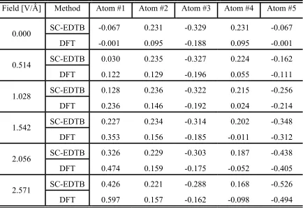
FIG. 2.2 Properties of a diamond cluster (insert) composed of 161 carbon atoms. (a) Spectrum given by the SC-EDTB method. The solid line denotes the SC-EDTB spec-trum for bulk diamond. Here and below the bulk specspec-trum is normalized to give the total number of states equal to the number of carbon valence electrons. In addition to the bulk spectrum was shifted by -2.9 V, the average Coulomb potential experienced by carbon atoms in the cluster (cf. Fig. 2.2(b)). (b) Coulomb potential profile along the <001> and <111> lines passing through the center of mass of the cluster. The vertical lines mark cluster facets. Right insert shows the radial density distribution (the product of density and squared radius) for s and p-orbitals.
Valence Electron Eigenvalues (eV)
To optimize a, , , and , a TF is built that fits MP’s and eigen-value spectra for benzene, methane, and ethane. The TF also includes a subfunction for fitting MP’s in a small hydrogen-passivated diamond cluster with {111} and {100} fac-ets.19 Spectra moments fitting for benzene and eigenlevel fitting for methane and ethane is performed. Methane levels can be unambiguously identified by their degeneracies; the (un)occupied portion of the methane spectrum has one nondegenerate and one triply de-generate level (cf. Fig. 2.3). The ethane 14x14 SC-EDTB Hamiltonian matrix can be broken into , which includes all but the diagonal SC correction elements and non-self-consistent EDTB matrix plus diagonal SC correction elements:
EHOnSite
G
SSσ SPσ
HSC NonDIA
H = HEDTB SCDIAG+ + HSC NonDIAG .
(2.10) Fortunately the secular equation for can be solved analytically.20 A par-ticular set of parameters a, , , and is substituted into the analytical ex-pression for a certain eigenenergy level, its numerical value is obtained, and the SC-EDTB wave function corresponding to this level is identified. Then by analyzing the wave function symmetry it is matched to its DFT counterpart. This determines which numerical DFT level should be matched to the given SC-EDTB analytical eigenenergy expression. The analytical solution establishes links between DFT and SC-EDTB levels by using just one particular parameter set, though these links are valid for any set of a,
, , and .
HEDTB SCDIAG+
SSσ SPσ
EHOnSite
EHOnSite SSσ SPσ
SC-EDTB counterpart (given by the corresponding analytical eigenvalue expression for ) is evaluated. The numerical solution gives a SC Hamiltonian matrix, and hence . Treating as a small perturbation, the first order cor-rection to is obtained. Then the ethane energy levels target subfunc-tion EthaneTsubF is calculated as
EiSCEDTB
IAG
EiSCEDTB HEDTB SCDIAG+
HSCNo δEiSCEDTB
nD HSCNonDIAG
Et
i
∑
haneTsubF a Weight E
E
i iDF
SS SP Ei
, OnSite, ,
SCEDTB
σ σ
− +
EHOnSite
(
)
(
)
[
]
H
Ei E
T SCEDTB
Shift .
δ
=
+ 2 (2.11)
The optimized values of a, , , and are given in Table 2.4. These values along with those from Table 2.1 were used to obtain molecular (Fig. 2.3) and hydrogen-passivated diamond clusters spectra (Fig. 2.4
SSσ SPσ
).
TABLE 2.3 Dipole moment and energy decrease for a C5 linear chain when it is placed
in a 2.571 V/Å external electric field.
SC-EDTB DFT Relative Error
Dipole Moment 2.51 e×Å 3.60 e×Å 30%
Energy Decrease -3.21 eV -4.56 eV 30%
TABLE 2.4 Optimized hydrogen orbital exponential coefficient [Ǻ-2], and C-H bond parameters [eV].
a EHOnSite SSσ SPσ
2.74101 3.52045 -3.33111 5.49273
Orbital shape discrepancies account for an erroneously large potential drop at the free diamond surface, and hence for wrong electron affinity (EA) values. The EA for a clean diamond {111} surface obtained by using the SC-EDTB model is 2.7 eV. This value can be confirmed by Fig. 2.2(a), which shows a slightly higher EA because in addi-tion to eight {111} facets the cluster has two {100} facets. Dimensional effects are not essential for a cluster of that size.
hydrogen-ated surface are -1.2 eV, -1.4 eV, and -2.03 eV, respectively. As noted in [21] only the EA difference between clean and passivated surfaces can be calculated reliably, while absolute EA values may contain large errors. Hence
∆EA
∆EA is the major quantity that should be used to compare SC-EDTB to DF calculations. ∆EA values for DFT and SC-EDTB are 2.53eV and 3.9eV, respectively
The incorrect free surface EA is considered an important drawback of our parameterization. Note, however, that if a non-self-consistent EDTB is used, the values of the free surface EA will be about 20-30 eV regardless of the orbital shape. All other SC-EDTB tests seem to give a reasonably good fit to DF data.
TABLE 2.5 MP’s for carbon atoms in hydrocarbon molecules.
Methane Ethane Benzene
SC-EDTB DFT SC-EDTB DFT SC-EDTB DFT
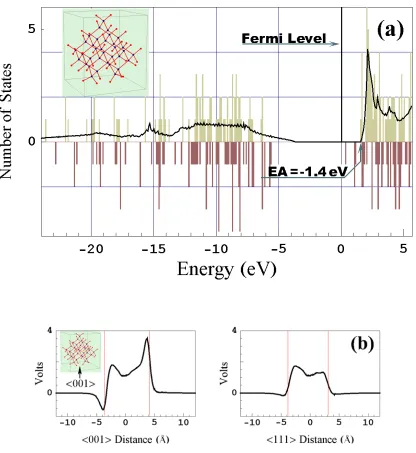
FIG. 2.4 Properties of a hydrogen-passivated diamond cluster (insert) composed of 34 carbon atoms. (a) SC-EDTB (top) and DF (bottom) spectra. In addition to the bulk spectrum (solid line) was shifted by 1.6 V average Coulomb potential experienced by carbon atoms in the cluster (cf. Fig. 2.4(b)). Note that the DF underestimates the band-gap for bulk diamond by approximately 1.0 eV. (b) Coulomb potential profile along <001> and <111> lines passing through the center of mass of the cluster. The vertical lines mark cluster facets.
2.4 PROPERTIES OF NANODIAMOND CLUSTERS RELATED TO FIELD EMISSION
As a demonstration of the method described in the previous sections, properties of nano-diamond (ND) coatings in field emitter applications are explored. The simulations typically contained between 250 and 500 carbon atoms, and all simulations were done on a low-end workstation (500 MHz dual Pentium III Xeon).
There is experimental evidence23 that ND coatings deposited on Si needle-shaped field emitters substantially lowers emission threshold voltages relative to that of bare Si needles and needles with micro-diamond powder coatings. ND coatings are created ei-ther by bias enhanced microwave plasma chemical vapor deposition24 or by
emission mechanisms that are explored are called the Inhomogeneous and Homogeneous Emission Models (IEM and HEM) , respectively.
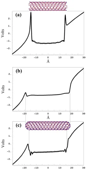
FIG. 2.5 Illustration of Inhomogeneous Emission Mechanism. (a) Schematic diagram of an infinite hydrogenated diamond surface with a small unpassivated metallic patch. (b) Potential for the infinite dipole layer containing a circular hole. (c) Potential experienced by an electron in vacuum in the vicinity of a round unpassivated metallic patch when a uniform external field is applied normally to the dipole layer. The force field line origi-nating from the patch edge shows the classical trajectory for an emitted electron.
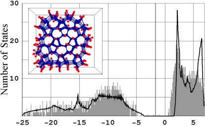
FIG. 2.7 Eigenvalue spectrum for a hydrogen passivated 5-7 membered ring ta-C cluster composed of 276 carbon and 168 hydrogen atoms (insert). To account for an EA = -1.4 eV the bulk diamond spectrum (solid line) is shifted by 1.4 eV.
equally between the two barriers. Experimental studies27 indicate that the degree of
amorphization of tetrahedrally coordinated amorphous carbon (ta-C) can be used for tun-ing the band gap size between 5.5 eV and 0.5 eV. The case that resembles Fig 6(c) was implemented for these calculations. A zero EA eigenvalue spectrum for a hydrogen pas-sivated ta-C cluster composed of 5-7-membered rings is plotted in Fig. 2.7.
________________________________________________________________________
sur-face is -1.75 eV and just 0.1 eV below Fermi level. That defines point H in the band structure diagram.
________________________________________________________________________
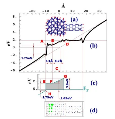
FIG. 2.9 IEM simulation: (a-b) System used to analyze IEM and wave functions with the energies belonging to the interval [EF,EF+0.5 eV]. The circle sizes are proportional
Note that although the standalone ta-C cluster exhibits an almost zero EA (Fig. 2.7), the system composed of the ta-C cluster and SWNT has a negative EA. This is due to the edge effect, i.e. plateau EF, and because the ta-C cluster becomes negatively charged when it comes into electric contact with the metallic SWNT in an applied field. Hence its band structure is shifted towards higher energies and the EA becomes negative.
The one-dimensional WKB approximation
( )
[
( )
]
P E m V x E dx
a b
= − −
∫
exp 2 22
h
(2.12)
is used to estimate the tunneling probability through the barrier shown in Fig. 2.8(c) as
PHEM = − ∫ + − x dx− ∫ dx
= × −
0 36 165 30 165
8 2 165
35 10
0 8 2
0 5 1
9
. exp . . .
. .
.
. .
(2.12a) For evaluation of Eq.(2.12a), m is assumed to be the electron mass in vacuum.
calcu-lated that originate from the grid points on the surface of spheres centered on the surface atoms of the cluster. The tunneling probability is calculated from Eq.
(2.12) for each field line using integration along the field line instead of a one-dimensional integration. The force line corresponding to the highest tunneling probabil-ity is selected. The grid point on the sphere surrounding the particular atom where the optimal field line originates is considered the emission site. In Fig. 2.9 the emission site is marked by point A and the optimal field line AD is indicated. Point D corresponds to the potential equal to the Fermi energy, i.e. electron motion along the field line beyond point D corresponds to a positive electron energy. Note that the field line has a sharp bend towards the hydrogenated surface near the emission site. This is similar to the one shown in Fig. 2.5(c), and is considered an IEM hallmark. Point A is not well defined; it is chosen here to lie on the sphere with a 1.0 Å radius. Plotted in Figure 2.9(d) is the radial density distribution for the surface atom where the optimal field line originates. The den-sity is plotted along the line connecting point A and the nucleus of the emission atom (in Fig. 2.9(d) it has coordinate –1.0). As seen from the plot, the density at A is one third of the peak density, which is assumed to be sufficient for emission. Applying Eq.
(2.12) to the barrier shown in Fig. 2.9(c) results in a tunneling probability equal to 4.1×10⁻⁵, which is four orders of magnitude higher than the HEM case. If the optimal field line is started from the nucleus rather than point A, the tunneling probability will decrease by a factor of 20. That, however, does not change the prevalence of the IEM over the HEM for tunneling probability in ND coatings.
(2.12) to the barrier inside the ND or ta-C particle is not well determined. The electron effective mass in semiconductors can be used only in the vicinity of the CB edge because the idea of effective mass is based on the periodic nature of Bloch functions. When the electron energy is 1.6-3.0 eV below the CB edge, instead of periodic oscillations the wave function exhibits a strong exponential decay and the concept of effective electron mass becomes invalid. That is the reason for using an effective mass equal to unity for estimating the HEM tunneling probability. However, it is interesting to note that in this example the HEM and IEM tunneling probabilities become equal when the electron ef-fective mass in Eq.
(2.12) equals 0.27. The reported effective electron mass values for diamond substantially differs from those for ta-C. The experimental analysis of drift velocity in diamond28 gives 0.36 and 1.4. Similar values for diamond were obtained from DF local density approximation simulations (
m⊥ = m|| =
m⊥ = 0.26 and m|| = 1.50).29 On the other hand the study of blue shift variations in ta-C superlattices with respect to quantum well thick-ness30 gives a much smaller averaged effective mass mave = 0.067.
emis-sion. Note that a 0.21 V/Å applied field, which we used solely for demonstration pur-poses, is difficult to achieve even with a strong field enhancement at a Si needle tip. Ex-perimental setups23,24 result in a much smaller barrier tilt than is schematically shown in Fig. 2.6.
The chains of unpassivated islands act like atomically thin metal whiskers. Be-cause field enhancement is proportional to aspect ratio, such whiskers may significantly increase the extracting field. This idea is illustrated by Fig. 2.9(f), which shows the Cou-lomb potential along line BC (Fig. 2.9(a)) that passes in close proximity to the SWNT and to the surface conducting channel. The potential of the conducting channel is the same as the potential of the SWNT. At the same time the Coulomb potential around the channel, both in vacuum and in the semiconducting cluster, changes in a linear fashion. Strong field enhancement can be seen from Fig. 2.9(e). The potential at the emitting atom is much higher than the potential one interatomic distance apart. Note that the emission site in Fig. 2.9(e) looks like an isolated high potential region because other at-oms constituting the conduction strip are below the cross-sectional plane.
2.5 SUMMARY
dia-mond surface. All other SC-EDTB results fit DF and experimental data reasonably well. To illustrate SC-EDTB capabilities, field emission properties of metallic (hydro)carbon systems were considered. The calculations indicate prevalence for the inhomogeneous over homogeneous emission mechanism for ND coatings.
3. CONVERGENCE ACCELERATION SCHEME FOR
SELF-CONSIS-TENT ORTHOGONAL-BASIS-SET ELECTRONIC STRUCTURE
ME-THODS. EQUILIBRIUM CASE.
3.1 REVIEW OF CONVERGENCE ACCELERATION SCHEMES
An efficient convergence scheme is an essential part of any self-consistent (SC) electronic structure method. At present there is no universal convergence acceleration algorithm that fits all possible situations, and therefore a variety of algorithms have been developed. These various schemes differ in the types of systems for which they can be efficiently used, the scaling with respect to the number basis functions, and whether con-vergence is guaranteed. Some of the properties of existing SC concon-vergence algorithms are summarized in Table 3.1. All methods employing scalar function minimization have quadratic scaling per iteration if an orthogonal basis set is used. Scaling does not account for eigenproblem solving that always scales cubically for the systems considered here. Therefore the total number of flops per SC iteration is O(N3) plus the appropriate table value which indicates the price of “charge mixing”.
met-rics algorithms by Broyden-Fletcher-Goldfarb-Shanno (BFGS)37,34,35 or Davidson-Fletcher-Powell (DFP).37 The second category encompasses algorithms that minimize charge density or potential deviations from their self-consistent values38-40 by solving a system of nonlinear equations. These methods involve the evaluation of either an exact8 or an approximate39,40 Jacobian to solve a system of non-linear equations for charge den-sity components by using a Newton-Raphson algorithm.
TABLE 3.1 Properties of major SC convergence acceleration algorithms. The last col-umn gives the number of flops required to calculate the input charge density for the
(k+1)th iteration provided the kth iteration eigenproblem has already been solved.
M et ho d C at egory
Method Convergence Number of iterations
Number of iterations for metallic systems
Scaling for a single iteration: Orthogonal /
Nonorthogonal basis
Level Shifting Guaranteed for large level shift parameter
Medium or Large
May converge slowly O(N 2)/O(N 3)
DIIS May diverge Medium - O(N 2)/O(N 3)
Variable Metrics
BFGS or DFP
Guaranteed Medium Second order approxi-mation is not efficient
O(N 2)
S ca la r F un ct io n Mi ni mi zat ion
RCA
Guaranteed for Uniform Well Posed Systems
Medium May be large O(N 2)/O(N 3)
Broyden Guaranteed Large O(N) Large O(N) O(N 2)
Sol
vi
ng a Syst
em of nonl in ear equat ions Newton-Raphson for system of nonlinear equations
Each convergence acceleration method has its strengths and drawbacks. The con-vergence of level shifting algorithms depends on the value of the level shift parameter. The level shift parameter is not a priori known and should be individually optimized for each particular problem. It can be chosen large enough to provide a sufficiently large convergence radius and to guarantee convergence from the given starting point. How-ever, the level shift parameter cannot be chosen to be too large because the convergence rate is inversely proportional to the level shift parameter magnitude. For metallic systems the level shift parameter should be chosen sufficiently large to achieve enough separation between the HOMO and LUMO. That may result in inefficiencies in the first-order per-turbation approach, and hence slow convergence.
Recently Cancès and Le Bris32,33 introduced a new class of relaxed constraints algorithms (RCA). They provided a rigorous mathematical proof of convergence from any starting point provided the system is uniform well posed, i.e. the system has a finite HOMO-LUMO gap. As follows from the proof, the number of iterations towards self-consistency is inversely proportional to the HOMO-LUMO distance. Thus RCA, or at least its variants described in [32,33] may be inefficient when applied to metallic sys-tems.
The DIIS algorithm is superseded by the RCA in a sense of robustness, but may be slightly faster than the simplest RCA variant called the optimal damping algorithm. DIIS still remains popular for mostly historical reasons; it was introduced almost a dec-ade prior to RCA. We put no comments on “Number of iterations for metallic systems” in Table 3.1 because there is no proof of convergence for DIIS, and thus its behavior for metals cannot be predicted.
Solving a system of non-linear equations for charge density components with an exact Jacobian is more efficient in terms of the number of required iterations than scalar target function minimization. This is because the Newton-Raphson algorithm for the sys-tem of equations drives each charge density component during each iteration step towards its self-consistent value. Scalar target function minimization does not possess this prop-erty. While a scalar target function (e.g. total energy) is driven to its minimum, some of charge density components may deviate further at each step from their self-consistent values.
of a single SC iteration, which is also used to improve an approximate Jacobian by the Broyden method,8,9 is an O(N2) flops operation.10 However O(N) iterations are required to build up an approximate Jacobian that is sufficiently close to the real one. The Broy-den algorithm is best suited for use in conjunction with O(N) methods for energy minimi-zation. However, the Broyden method is not a good candidate for metallic systems for which O(N) energy minimization11,12 cannot be efficiently applied because the localiza-tion range of Wannier-like orbitals is larger than the typical system size.
system size no worse than O(N3). In addition, a convergence scheme that is applicable to transport problems is desirable, and thus the algorithm framework should in principle be extendible to non-equilibrium cases.
We demonstrate our scheme using an environment dependent tight binding (EDTB) methodology combined with self-consistent (SC) field corrections.3 The EDTB approach effectively includes three-center integrals through the dependence of hopping integrals on their atomic environment, resulting in a method that in many cases can pro-duce results that are superior to DFT schemes with the same number of basis functions per atom. The self-consistent corrections involve adding block-diagonal matrix elements ∆H to the tight-binding Hamiltonian matrix. The matrix ∆H is sparse, with its elements ∆Hαβ being zero if indexes α and β do not belong to the same atom (though α and β may
stand for different orbitals of the same atom for non-zero ∆Hαβ). The method for
com-puting ∆H, which involves using an explicit minimal Gaussian basis set, is described elsewhere.43
3.2 NEWTON-RAPHSON METHOD FOR NONLINEAR SYSTEMS OF EQUATIONS
The Newton-Raphson method1 belongs to the class of globally convergent meth-ods, where convergence is guaranteed regardless of the initial charge density guess. The idea of the algorithm is the following. For the non-self-consistent set of Kohn-Sham equations, some input electron density ρin determines the Hamiltonian matrix H and hence output electron density
( )
( ) ( )
{ }
ρ ϕα ϕβ α
α β α β
out r r r i
i N N
=
= = =
∈
∑
∑
1SameAtom, 1 1 ,
β f Ci Ci
[ ]
fi ≡ f εi =
[
1+exp(
ε µi−)
]
−1kT .
(3.1a) Here ϕζ is the atomic orbital, Ci is the component of the ith eigenvector of ma-trix
ζth
ζ ζth
H = H
[
ρin]
, and εi is the ith Hamiltonian eigenvalue. Because orbital orthogonalityis assumed, Eq.(3.1a) contains only the products with indexes α and β belonging to the same atom.
Further we operate with uncompensated Mulliken populations qαβ =2
∑
iN=1/2Ci Ciα β −q0α αβδ if T = 0(3.1b)
qαβ =2
∑
iN=1f Ci Cii α β −q0α αβδ if T > 0(3.1c) rather than electron densities. Here δαβ is the Kronneker delta, and q0 is the orbital Mulliken population in the bulk material for which a TB parameterization (in this case the EDTB parameterization) has been performed.13 For example 1.2028 if
α
α =
q0 α
equi-librium value, i.e. a measure of the deviation from neutrality. Because indexes α and β belong to the same atom, matrix is sparse and further is treated as a double indexed vector. If we apply a small change
qαβ
∆qInαβ to input vector it will result in a small change
qInαβ
δH of the Hamiltonian H and a small change ∆qOutαβ of output vector qOut . If is infinitesimally small, we can relate it linearly to
αβ
∆qInαβ δHαβ. This in turn can be
related to ∆qOutαβ in a linear fashion using first order perturbation theory
{ }µ ν , ∈ µ ν 2 , αβ µ ν N =
∑
, =SameAto1 1
{ } A N µ= ν= ∈
∑
1, 1 Same qIn µν αβ H β q
∆qInαβ
qOutαβ + ∆ qInαβ
qOut
qOut ν qIn qIn
Atom αβ µ αβ = + ∆ ∆ , .
δHαβ = U ,µν µν
m
∆ , (3.2a)
∆qOutαβ = αβ µν, δH
Atom
.
(3.2b)
To make further calculations more convenient, we do not include the spin factor of 2 into matrix A. Due to the atomic orbital’s orthogonality, the change of Hamiltonian matrix δ is applied only to the elements with indexes α and belonging to the same atom. That allows us to view δHαβ as a vector with the same length as . If we want the self-consistency condition to be valid we must apply
αβ
such that the output charge density qOutαβ equals + ∆qInαβ:
Matrix B is a product of U and 2 A as defined by Eqs.(3.2a). During each iteration step we use Eq.(3.3) to obtain the additional contribution of ∆qInαβ to the current iteration charge input vector qInαβ. Vector ∆qIn is a solution of a linear system
(
E−B)
∆qIn qOut qIn= − ,(3.4) where E is the identity matrix.
If the exchange energy is represented as a first order expansion over Mulliken population deviations from their bulk values, the matrix U is the same for each iteration. Its evaluation requires computation of Hartree and exchange integrals. These integrals can be evaluated analytically for Gaussian basis functions in O(N2) flops. The main computational burden is imposed by the evaluation of matrix A. As will be shown in Section 3.3 the exact evaluation of A, which is an O(N4) operation, can be substituted by the approximate evaluation. In contrast to the Broyden method the approximate Jacobian Aαβ µν, =∂δ µνH ∆qOut is not calculated iteratively. Instead a new value of is computed during each iteration. Its evaluation requires about 4N3 flops. Remarkably, precision in a wide range is not related to computational workload. For sufficiently large systems the precision enhancement from 10-2 to 10-3 leads to O(N2) extra operations. According to our experience if the maximum deviation of approximate matrix A elements from their exact values is around 10-2, any further precision enhancement does not accel-erate the convergence.
A= A qIn
[
]
in Mulliken population. The former is achieved by ODA after 24 iterations, while it takes 4 iterations for the Newton-Raphson algorithm to achieve a 10-5 Mulliken popula-tion convergence.
Another reason for developing a Newton-Raphson based scheme is its applicabil-ity to non-equilibrium situations. None of the scalar target function minimization tech-niques will work for non-equilibrium cases because SC non-equilibrium electron densi-ties do not correspond to a global energy minimum. At the same time the matrix
Aαβ µν, =∂δ µνH ∆qOut can still be readily evaluated for non-equilibrium systems, which means that the analogue of the Newton-Raphson scheme presented here can be used for non-equilibrium studies.
3.3 IMPROVED SCALING FOR THE NEWTON-RAPHSON ALGORITHM
The key equation (3.2b) employed by the Newton-Raphson method relates the in-finitesimally small change of the Hamiltonian matrix δH to the induced changes of Mul-liken population components. We first consider this equation assuming zero temperature and a nondegenerate HOMO, which implies a finite HOMO-LUMO gap ∆. In section 3.4 it is extended to finite temperatures and metallic systems that may have degenerate HOMOs. The symbol H0 is used to denote the unperturbed Hamiltonian matrix, C0 de-notes a matrix with columns that are H0 eigenvectors, and C0i and ε0i denote the ith column of C0 and the ith eigenvalue of H0, respectively. For zero temperature and a non-degenerate HOMO the component of the uncompensated Mulliken population vector is given by (3.1b). The variation of caused by the variation of the Hamiltonian ma-trix
qαβ
(
)
(
)
∆q C0i C0 Inv C0 H C0i C0i C0 Inv C0 H C0i
i T i N i T i N αβ α β β α ε δ ε δ = = + =
∑
∑
2 2 1 2 1 2 / / . (3.5)Here the superscript “T” denotes a transposition, and
( )
...ζ indicates the ζth component of the expression in the parenthesis. The symbolεInvi stands for a diagonal matrix that has(
ε0i −ε0j)
−1 at the jth position if ε0i ≠ε0j, and 0 otherwise. Equation (3.5) is simi-lar to the one used by Brown8 who first proposed using the Newton-Raphson algorithm for SC convergence acceleration. We provide a derivation of (3.5) in the Appendix A. This is done for two reasons. First, it systematically handles the case of degenerate en-ergy levels. Second, the intermediate equations obtained during the derivation are crucial for understanding the finite temperature case presented in Section 3.4.To estimate the number of flops with respect to the number of orbitals N required to evaluate Eq.(3.5), one needs to switch from a matrix notation to an explicit summation over matrix indexes. For brevity we consider only the first sum in Eq.(3.5). Here
(
εInvi mm)
is the mth diagonal element of εInvi.(
)
C0i C0 Inv C0 H C0ii T i N α ε δ β = =
∑
1 2 /(
)
C0i C0m Inv C0m C0i H
m N
N
i mm n s
i N s N n N ns α β ε δ = + = = =
∑
∑
∑
∑
( / ) / 2 1 1 2 1 1 . (3.6)Because δH is sparse, the double summation over indexes n and s requires order of N flops. If the system is composed solely of carbon atoms and we assume four orbitals per atom, there are ten distinguishable combinations of index pairs {α,β}, and {n,s} per atom. Therefore the expression in the parenthesis in Eq.(3.6) can be viewed as a square matrix (further on we refer it as matrix A) with dimensions 2.5N, and double indexing {α ,β}, and {n,s} in each dimension. The term
(
εInvi mm)
couples the summation over indexes i and m. Because the summation over i and m can not be performed separately, N 2 flops are required to evaluate each entry of A, and (2.5N)2N2 flops are required for the evaluation of the entire matrix. To decouple the summation over i and m, and thus switch from N 4 to N 3 scaling, we substitute(
εInv)
i mm by its power approximation. To
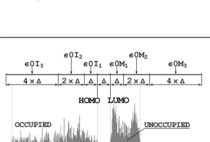
demonstrate the basic idea let us consider the sample spectrum and its partitioning illus-trated in Fig. 3.1. The centers of the energy intervals for occupied and unoccupied parts of the spectrum are marked as ε0Ix or ε0Mx, respectively. For each given ε0i and ε0m which belong to the intervals with centers at ε0Ix or ε0My respectively, the value of
(
)
ε0I m− ε ε 0M 0m x y y − 1 1 ε ε 0 0 0 0I i x = ε ε ε 0 0 0M i m x y = −(
)
ε0 ε0 ε
ε ε
I
0M
− − −
ε0My
−
0m
x y
(
εInv)
(
)
(
)
ε ε ε Inv ii mm −
× + − − 1 1
(3.7)
can be approximated by a Taylor expansion over a small parameter
λ =
(
)
0I
i x
. (3.8)
(
)
(
)
A C0i C0m C0m C0i0 0I 0 0M
n s
m N N
i N
xy jk i x
j
m y
k k
j
j y i Int
Y
x m Int X
x y
≈ ×
− −
= + =
= − = ∈ ∈
∑
∑
∑
∑
∑
∑
α β
ε ε ε ε .
/ /
, ,
,
2 1 1
2
0 3 0 3
Λ
(3.9)
FIG. 3.1 Sample semiconductor spectrum and energy axis partitioned for the use with Eq.(3.9). For better efficiency of approximation Eqs.(3.9-3.11) (un)occupied intervals can be shrunk proportionally to the size of the (un)occupied portion of the spectrum.