ABSTRACT
BARNARD, EMILY SARAH. The Canonical Join Representation in Algebraic Combinatorics. (Under the direction of Nathan Reading.)
We study the combinatorics of a certain minimal factorization of the elements in a finite lattice L called the canonical join representation. The join ⋁A=w is the canonical join rep-resentation of w if A is the unique lowest subset of L satisfying ⋁A = w (where “lowest” is made precise by comparing order ideals under containment). When each element in L has a canonical join representation, we define the canonical join complex to be the abstract simplicial complex of subsets A such that ⋁A is a canonical join representation. In the first chapter, we characterize the class of finite lattices whose canonical join complex is flag, and show how the canonical join complex is related to the topology ofL.
Next, we study the canonical join complex of the Tamari lattice in types A and B. We realize the canonical join complex of the Tamari lattice as a complex of noncrossing arc diagrams, give a shelling order on its facets, and show that it is homotopy equivalent to a wedge of Catalan-many spheres. We extend these results to thec-Cambrian lattices of type A, which we show to be vertex decomposable.
© Copyright 2017 by Emily Sarah Barnard
The Canonical Join Representation in Algebraic Combinatorics
by
Emily Sarah Barnard
A dissertation submitted to the Graduate Faculty of North Carolina State University
in partial fulfillment of the requirements for the Degree of
Doctor of Philosophy
Mathematics
Raleigh, North Carolina 2017
APPROVED BY:
Patricia Hersh Ricky Liu
Seth Sullivant Nathan Reading
DEDICATION
BIOGRAPHY
ACKNOWLEDGEMENTS
The author thanks her advisor, Nathan Reading, for his editorial suggestions and helpful con-versations. She thanks her committee members: Patricia Hersh (who suggested the connection to the crosscut complex in Chapter 2), Ricky Liu, Blair D. Sullivan, and Seth Sullivant.
The author thanks the many other mathematicians whose conversations have shaped this document for the better: Andrew Carroll, Al Garver, Emily Gunawan, Christophe Hohlweg, Alexander Martsinkovsky, Thomas McConville, Victor Reiner, David Speyer, Gordana Todorov, and Shijie Zhu. This includes the fellow and former members of the Reading research group: Erin Bancroft, Chetak Hossain, Shirley Law, Emily Meehan, Salvatore Stella, and Shira Viel. She thanks her delightful and encouraging officemates, and the insightful crew at the graduate algebra and combinatorics seminar.
TABLE OF CONTENTS
List of Tables . . . vii
List of Figures . . . viii
Chapter 1 Introduction . . . 1
1.1 The canonical join representation . . . 1
1.2 The combinatorics of the canonical join representation . . . 2
1.3 Finite Coxeter groups . . . 4
1.4 The topology of the canonical join complex . . . 6
1.5 Coxeter-biCatalan combinatorics . . . 7
Chapter 2 The Canonical Join Complex . . . 9
2.1 Introduction . . . 9
2.2 Motivation and examples . . . 12
2.3 Finite semidistributive lattices . . . 14
2.3.1 Definitions . . . 14
2.3.2 The flag property . . . 18
2.3.3 Crosscut-simplicial lattices . . . 26
2.4 Lattice-theoretic constructions . . . 29
2.4.1 Sublattices and quotient lattices . . . 29
2.4.2 Products and sums . . . 30
2.4.3 Day’s doubling construction . . . 31
2.5 Discussion and open problems . . . 36
Chapter 3 The Canonical Join Complex of the Tamari Lattice . . . 40
3.1 Introduction . . . 40
3.2 Background . . . 42
3.2.1 Lattice-theoretic background . . . 42
3.2.2 The noncrossing arc complex . . . 44
3.2.3 Thec-Cambrian congruence and the Tamari lattice . . . 46
3.2.4 The type-B Tamari lattice . . . 47
3.2.5 Noncrossing perfect matchings . . . 49
3.3 Shellability of the Tamari lattices . . . 51
3.3.1 The Tamari lattice in type A . . . 51
3.3.2 The Tamari lattice in type B . . . 53
3.4 Vertex Decomposability of thec-Cambrian lattices . . . 63
3.4.1 Thec-Cambrian lattices . . . 63
3.4.2 Vertex decomposability . . . 64
Chapter 4 Coxeter BiCatalan Combinatorics . . . 76
4.1 Introduction . . . 76
4.2 BiCatalan objects . . . 80
4.2.2 BiCambrian fans . . . 84
4.2.3 The biCambrian congruence, twin sortable elements, and bisortable ele-ments . . . 88
4.2.4 Twin clusters and bicluster fans . . . 91
4.2.5 Twin noncrossing partitions . . . 94
4.3 Bipartite c-bisortable elements and alternating arc diagrams . . . 95
4.3.1 Pattern avoidance . . . 95
4.3.2 Noncrossing arc diagrams . . . 96
4.3.3 Alternating arc diagrams . . . 97
4.3.4 Counting alternating arc diagrams . . . 99
4.3.5 Enumerating bipartitec-bisortable elements in type B . . . 103
4.3.6 Simpliciality of the bipartite biCambrian fan in types A and B . . . 106
4.4 Double-positive Catalan numbers and biCatalan numbers . . . 110
4.4.1 Double-positivity . . . 110
4.4.2 Counting twin nonnesting partitions . . . 112
4.4.3 Canonical join representations and lattice congruences . . . 114
4.4.4 Canonical join representations ofc-bisortable elements . . . 118
4.4.5 Counting bipartitec-bisortable elements . . . 121
4.4.6 BiCatalan and Catalan formulas . . . 123
4.4.7 The double-positive Catalan numbers . . . 128
4.4.8 The Type D biCatalan number . . . 133
4.4.9 Type-D biNarayana numbers . . . 135
LIST OF TABLES
Table 4.1 TheW-biCatalan numbers . . . 78
Table 4.2 The biNarayana numbers . . . 79
Table 4.4 The type-D biNarayana numbers . . . 80
Table 4.6 Some double positive Catalan numbers . . . 128
LIST OF FIGURES
Figure 1.1 Any map φof from the setX to a latticeL extends uniquely to a lattice
homomorphism ˜φ∶F →L. . . 2
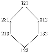
Figure 1.2 The weak order on the symmetric group S3. . . 5
Figure 2.1 The canonical join complex is an empty triangle. . . 10
Figure 2.2 Some examples of noncrossing arc diagrams. . . 13
Figure 2.3 Two finite lattices whose top elements have no canonical join representation. 15 Figure 2.4 Dashed lines represent order relations inLwhile solid lines represent cover relations. . . 18
Figure 2.5 Some order relations in the join-refinement order for L. . . 21
Figure 2.6 Some relations in the join-refinement order for L. . . 22
Figure 2.7 A depiction of the argument for Lemma 2.3.13. Dashed lines represent order relations in Lwhile solid lines represent cover relations. . . 24
Figure 2.8 An illustration of the argument for the proof of Corollary 2.1.5. Dashed gray lines represent relations in L while solid black lines represent cover relations. . . 25
Figure 2.9 A finite crosscut-simplicial lattice failing both SD∨ and SD∧. . . 26
Figure 2.10 Dashed lines represent relations inLand solid lines represent cover relations. 27 Figure 2.11 Dashed lines represent relations in L while solid lines represent cover relations. . . 28
Figure 2.12 The Tamari latticeT3 and its canonical join complex. . . 30
Figure 2.13 The canonical labeled join graph of three non-isomorphic congruence uni-form lattices. . . 33
Figure 2.14 The two leftmost graphs are isomorphic Hasse diagrams for the distribu-tive lattice L. Rightmost is the lattice obtained by doubling the interval [a, e] inL. . . 35
Figure 2.15 Doubling the interval [a, e] in the leftmost congruence uniform lattice yields the left-middle lattice, whose canonical join graph is isomorphic to C6. Doubling the interval [a, e] in the right-middle lattice yields the rightmost lattice, whose canonical join graph is isomorphic to C7. . . 36
Figure 2.16 Left: The weak order for the symmetric group S3. Right: The lattice of 2-multichains. . . 38
Figure 2.17 Left: The canonical join complex of weak order for the symmetric group S3. Right: The canonical join complex of the lattice of 2-multichains. . . 38
Figure 3.1 The Tamari lattice T3 and its canonical join complex. . . 40
Figure 3.2 The faces in the canonical join complex of the weak order onS3. . . 41
Figure 3.3 From left to right: δ(4123), δ(2413), δ(2341), andδ(3412). . . 45
Figure 3.4 Left: δ(2431). Right: The arc corresponding to the canonical joinand 2314. 46 Figure 3.5 A demonstration of the map µ. . . 53
Figure 3.6 Each diagram contains two symmetric arcs. . . 54
Figure 3.8 The nodes [k1, k2−1] are filled in with a maximal collection of ordinary
right arcs. . . 57
Figure 3.9 An illustration of the map µs when il≠ −1. . . 58
Figure 3.10 An illustration of the mapµs when il= −1. . . 58
Figure 3.11 An illustration of the first two steps for the mapν. We curve some of the edges in the matching M to make them more suggestive of the arcs they will become in ν(M). . . 59
Figure 3.12 An illustration of the mapν. . . 60
Figure 3.13 The arcsα1,7 and α2,8 in ∆(9,{4,5,8},{2,3,6,7}). . . 67
Figure 3.14 The arcα1,7 in ∆(9,{1,2,3,4,5,7},{6,8}). . . 69
Figure 3.15 The set {α3,5, α2,3} ∈ lk(α1,4), and it is a facet in ∆∖2(5,{4},{2,3}) ∖ {α1,5, α1,4}. . . 72
Figure 3.16 In ∆(9,{4,5,8},{2,3,6,7}), arcs α2,8 and α1,3 intersect. . . 73
Figure 4.1 Some doubled root posets . . . 81
Figure 4.2 Some posets of join-irreducibles of doubled root posets . . . 83
Figure 4.3 Cambrian fans and the biCambrian fan in type B2 . . . 85
Figure 4.4 The linear biCambrian fan in type A3 . . . 86
Figure 4.5 The bipartite biCambrian fan in type A3 . . . 86
Figure 4.6 The linear bicluster fan in type A3 . . . 93
Figure 4.7 The bipartite bicluster fan in type A3 . . . 93
Chapter 1
Introduction
1.1
The canonical join representation
Throughout mathematics, and algebra in particular, one sees the unique decomposition of an object into irreducible or indecomposable components. In number theory, this is the prime factorization of an integer; in commutative algebra, this is the primary decomposition of an ideal; and in representation theory, this is the direct sum decomposition of a representation into indecomposable representations. The organizing principle of this thesis is the lattice-theoretic analogue: the canonical join representation.
Recall that a lattice L is a partially ordered set such that each pair of elements w and v has a smallest upper bound, called thejoin, and a greatest lower bound, called the meet. We writew∨vor⋁{w, v}for the join ofwandv, andw∧vor⋀{w, v}for the meet. Alternatively, one can think of a lattice as a universal algebra, with operations (∨,∧) that are associative, idempotent, and satisfy the absorption laws: w∨ (w∧v) =w and w∧ (w∨v) =w. A lattice homomorphism is a map φ ∶L→L′ between lattices L and L′ that respects the meet and
join operations. We say that the image of φis alattice quotient of L.
X F
L ι φ
˜ φ
Figure 1.1: Any map φ of from the setX to a lattice L extends uniquely to a lattice homo-morphism ˜φ∶F →L.
for much of the research on free lattices [39, Section 2]. As a part of his solution, Whitman constructed an algorithm that transforms any given polynomial expression into a “shortest” form [44, Appendix G, Section 1]. It turns out that this expression is also the canonical join representation of the corresponding element, and it is minimal in an order-theoretic sense: In a general latticeL, the expression ⋁A is the canonical join representation of an elementwif it is the unique “lowest” irredundant expression forw as a join. One makes the notion of “lowest” precise by comparing order ideals. In this case, we also say that the set A is a canonical join representation (although, more precisely, we mean that⋁A is a canonical join representation). Later, J´onsson noticed a further connection between the algebraic structure of a lattice and this canonical form [53]. Certain elements in a lattice may not admit a canonical join representation. (For example, Figure 2.3 depicts two lattices, and in each the top element does not have a unique minimal expression⋁A.) When Lis finite, each element admits a canonical join representation if and only if the lattice also satisfies a certain weakening of the distributive law called join-semidistributivity:
If x∨y=x∨z, thenx∨ (y∧z) =x∨y. (SD∨)
We say that L is join-semidistributive if it satisfies SD∨ for each x, y, and z. If L also
satisfies the dual condition (where we replace ∨ with ∧) then it issemidistributive. For the remainder of this introduction, we assume thatL is finite and join-semidistributive.
1.2
The combinatorics of the canonical join representation
We focus our attention on the discrete structure of the collection ∆(L) of subsets A∈2L such thatAis a canonical join representation. Recall that anabstract simplicial complex ∆ on a set of verticesV is a collection of subsets of V satisfying: First,{v} ∈∆ for eachv∈V. Second, ifA∈∆ then each subsetA′⊂A also belongs to ∆. We call the collection of edges and vertices
in ∆ itsone-skeleton.
complex the canonical join complex of L. Its vertex set is the set of elements that cannot be written as a nontrivial join of lower elements. These elements are called join-irreducible. (That is,j is join-irreducible if j= ⋁A implies thatj∈A.)
As combinatorialists, we ask questions like:
• How many faces does the canonical join complex have? • What is the facial structure of the canonical join complex?
Because Lis finite and join-semidistributive, the answer to the first question is immediate: Each element admits a canonical join representation, so the number of faces is just the size of L. (The empty face is the canonical join representation for the smallest element.)
Answering the second question will be the main focus of Chapter 2, where we consider a certain combinatorial property called the flag property. See Theorem 2.1.1. A complex ∆ is flag if its minimal non-faces have size equal to 2. Informally, we can think of this condition as saying: There are no “hollow” simplices in ∆. More precisely, complex ∆ is flag if and only if it is determined by its underlying one-skeleton as follows: Given a set Aof vertices,A is a face in ∆ if and only if A is a clique in the one-skeleton for ∆.
The flag property appears at the intersection of combinatorics with graph theory, differential geometry, and topology. In particular, its connection to the Charney-Davis conjecture(s) [21] has received much attention. The Charney-Davis conjecture is essentially the polyhedral analogue to a classical conjecture of Hopf. Hopf’s conjecture relates the geometry and topology of a Riemannian manifold M, and states: If M has dimension 2n, and its sectional curvature is nonpositive, then(−1)nχ(M) ≥0, whereχ(M)is the Euler characteristic ofM. (Informally, the
sectional curvatureis the Gaussian curvature of the surface we obtain by taking two-dimensional slices of M. See [38, Conjecture 54].) When we further restrict to polyhedral flag complexes, the Charney-Davis conjecture has a purely combinatorial reformulation. See [38, Conjecture 72] or [63, Conjecture 1]. Next, we discuss a few familiar examples of flag complexes.
Example 1.2.1. Suppose that ∆ is a cell complex, and write BCS(∆) for the barycentric subdivision of ∆. Geometrically, we constructBCS(∆)by adding a vertexvF at the barycenter
of each face F in ∆. A subset of vertices {vF1, . . . , vFk} is a face if and only if it corresponds with aflag of faces F1⊂ ⋯ ⊂Fk in ∆. Clearly, each collection of vertices in BCS(∆) satisfies:
if each pair is a face, then the entire collection is a face. Thus,BCS(∆) is flag.
Example 1.2.2. LetP be a partially ordered set. Theorder complex forP is the simplicial complex whose k-dimensional faces are the chains x0 < ⋯ < xk. Suppose that each pair of
Example 1.2.3. Fix a convex polygonP, and consider the simplicial complex ∆(P)whose faces correspond to partial tilings ofP by triangles, so that its facets correspond to triangulations of P and its vertices correspond to the diagonals in P. It is well-known that this complex can be realized as the boundary of a convex polytope, called thesimplicial associahedron. Observe that a collection of diagonals belongs to a (partial) triangulation if and only if each pair in the collection does not cross. Thus, ∆(P) is flag.
1.3
Finite Coxeter groups
Many of the most interesting join-semidistributive lattices are closely related to theweak order
on a finite Coxeter group. We now turn our attention to the combinatorics of the canonical join representation in this context. In preparation for our results, we will give a gentle introduction to finite Coxeter groups and the weak order. (To find a complete discussion of finite Coxeter groups, with precise statements and proofs, see [12, 51].)
A Coxeter groupW is a group of transformations on Euclidean space, generated by orthog-onal reflections. The collection of reflecting hyperplanes is called theCoxeter arrangement for W, and it is fixed by the action of the group. Each finite Coxeter group is equipped with a special set of generators called simple generators, and these are typically a proper sub-set of all of its reflections. The group W has the following presentation in terms of its simple generatorss1, . . . , sn:
W = ⟨s1, . . . , sn∶ (sisk)mi,k =e⟩
The numbers mi,k are symmetric in iand k, and satisfy: mi,k ∈Z+∪ {∞},mi,k ≥2 wheni≠k,
and mi,i=1.
We encode this data with a graph called the Coxeter diagram that is defined as follows: Take the simple generators s1, . . . , sn as nodes, and connect si to sk whenever the number
mi,k ≥3. We typically label the edge{si, sk}by the numbermi,k whenever mi,k >3. A Coxeter
group isirreducible if its associated Coxeter diagram is connected. Finite irreducible Coxeter groups have been classified by their Coxeter diagrams. There are four infinite families—called An,Bn,Dn and I2(n)—and six exceptional types. Examples include the symmetry groups for
regular polytopes and the Weyl groups which appear in the study of semisimple Lie algebras. Below, we give two familiar examples.
Example 1.3.1. Consider the symmetry group W of an equilateral triangle drawn in R3,
so that its vertices are the standard basis vectors e1, e2, and e3. Each reflecting hyperplane
corresponds to an edge of the triangle as follows: The edge connecting ei and ek determines
an orthogonal plane, Hi,k = {x ∈ R3 ∶ xi = xk}, that cuts the edge in half and contains the
reader will recognize thatW is the symmetric groupS3 (orA2 in the Weyl group notation). In
general, we identify Sn with the symmetry group of the standard (n−1)-simplex. The simple
generators are the set of reflections corresponding to the adjacent transpositions. We usually write si for the transposition (i, i+1), where i∈ {1,2, . . . , n−1}. Thus, we havemi,i+1 =3 and
otherwise mi,k =2.
Example 1.3.2. Consider the symmetry group W of the regular n-cube, whose vertices inRn
are{(e1±⋯±en)}. The reflecting hyperplanes forW have normal vectorsei, ek±ei. We often
re-alizeW as the group of signed permutations. These are permutations on the set±{1, . . . , n} that satisfy the symmetry condition w(i) = −w(−i). In this permutation representation, each reflection corresponds either to a pair of transpositions (i, k)(−i,−k) or a “symmetric” trans-position(−i, i). The simple generators correspond to the transpositions(i, i+1)(−i,−i−1) and (−1,1), where i∈ {1,2, . . . , n−1}. We usually write s0 for the transposition (−1,1), andsi for
(i, i+1)(−i,−i−1). Thus, m0,1 =4, mi,i+1 = 3 for i >0, and mi,k =2 otherwise. In the Weyl
group notation, this is Bn.
We represent the elements of W as words in the simple generators S, although there are typically many such expressions for each element. The length l(w) is the size of a reduced, or shortest possible, expression for w. The weak order on W is defined by the cover relations w<⋅ws whenever l(w) < l(ws) and s ∈ S. Thus, the Hasse diagram for the weak order is just the Cayley graph for W (with generating set S). For each finite W, the weak order is a semidistributive lattice (see [26, Lemma 9]). In particular, each element has a canonical join representation.
123 132 213
312 231
321
Figure 1.2: The weak order on the symmetric groupS3
Example 1.3.3. Returning to the symmetric group Sn, from Example 1.3.1, we can describe
the weak order as follows: Write each permutation inSn in its one-line notation asw1w2. . . wn,
wherew(i) =wi. Acting on the right by the transposition(i, i+1) corresponds to swapping the
entries wi and wi+1. Thus, one moves up in the weak order by swapping adjacent entries that
1.4
The topology of the canonical join complex
In Chapter 3, we study the canonical join representation in certain lattice quotients of the weak order. These lattice quotients inherit semidistributivity, so each element admits a canonical join representation.
We begin by considering the Tamari lattice. The Tamari lattice is named for Dov Tamari, who proved that it is a lattice [40, 50], and defined it as follows: Consider a fixed word a1a2. . . an+1 and all of the possible ways to properly distribute brackets among its letters. We
think of the bracketing as defining a binary operation, where each (rightward) application of the associative law corresponds to a cover relation. For example, the Tamari latticeT2 consists
of the single cover relation (a1a2)a3 <⋅ a1(a2a3).
Since its original definition, the Tamari lattice has made surprising appearances in algebra, topology, category theory, and even physics (not to mention combinatorics) [59]. Appropriately, it has many realizations. It is convenient for us to realize Tn as the lattice quotient of the
weak order on Sn consisting of the permutations that avoid the pattern 312. We say that
a permutation avoids the 312-pattern if, for each pair of numbers i < k that appear out of order in w1. . . wn, we have that each j ∈ {i+1, . . . , k −1} precedes i and k. The Hasse
diagram for Tn is an orientation of the one-skeleton of a polytope. This polytope is the simple
associahedron—the dual (or polar) polytope of ∆(P) from Example 1.2.3.
Remark 1.4.1. The canonical join representation “sees” the geometry of the Hasse diagram forTn. More precisely, for any finite join-semidistributive lattice, there is a bijection from the
set {y ∶ w ⋅>y} to the canonical join representation of w. (This is Proposition 2.2.2.) Similar constructions were used to study the cover relations in free lattices. (See [39, Theorem 3.5].) When the Hasse diagram for L is the dual graph for a simplicial sphere ∆, as it is for the weak order and the Tamari lattice, the f-vector for the canonical join complex is equal to the h-vector for ∆.
Informally, a complex ∆ is shellable if we can linearly order its facets F1, . . . , Fm so that
when we glue Fi into the complex ⋃i−1r=1Fr of earlier facets, one of two possible events occurs:
Either the topology of the resulting complex does not change; or we close off a sphere of dimension∣Fi∣ −1. In Chapter 3, we show that the canonical join complex ofTnis shellable. See
Remark 1.4.2. The canonical join complexes that we study here are all non-pure, meaning that their facets have different dimensions. We use the notion of non-pure shellability developed by Bj¨orner and Wachs in [13] and [14]. As an immediate consequence, we also obtain a direct-sum decomposition of the associated Stanely-Reisner ring that generalizes the Cohen-Macaulay property of pure complexes. See [14, Theorem 12.3]. Historically, the connection to the Cohen-Macaulay property was a major impetus behind the study of shellable complexes [13].
1.5
Coxeter-biCatalan combinatorics
In Chapter 4, we use the canonical join representation to solve an enumerative problem at the heart of Coxeter-biCatalan combinatorics. Before we outline our results, we make a very brief introduction to Coxeter-Catalan combinatorics. A more complete history and discussion of examples can be found in [2] and [33].
Our story begins with the classicalCatalan numbers
Cn=
1 n+1(
2n n).
The study of the Catalan numbers dates back at least to Euler, who considered the problem of enumerating the triangulations of a fixed convex polygon [60]. Since that time, the Catalan numbers have appeared throughout algebraic combinatorics and enumerate more than 200 different combinatorial objects [83, Introduction]. Below, we call such an object a Catalan object.
Example 1.5.1. Our touchstone example is the Tamari lattice Tn. Recall that the Hasse
diagram for the Tamari lattice can be realized as the one-skeleton for the simple associahedron. Since the vertices for the simple associahedron are parametrized by the triangulations of a fixed convex polygon, we conclude that there are Catalan many elements inTn.
In Coxeter-Catalan combinatorics, many of the traditional Catalan objects are seen as a special case of a general construction. This general construction yields a Coxeter group analogue for each of the traditional Catalan objects. So, for example, each Coxeter group has its own version of the Tamari lattice. (More precisely, each Coxeter group has a family of Tamari-like lattices.) See Example 1.5.2. In general, this construction depends on a choice of a Coxeter groupW, a set of simple generatorsS, an orientationcof the Coxeter diagram (c is also some-times called a Coxeter element), and a collection of vectors Φ related to the combinatorics of the Coxeter arrangement.
Example 1.5.2. Recall that the Tamari lattice Tn is the lattice quotient of the weak order
case of a more general lattice quotient construction that can be applied to the weak order on
any finite Coxeter group. This general construction yields the so-calledc-Cambrian lattices, a family of lattice quotients parametrized by an orientationcof the associated Coxeter diagram. In particular, whencis an orientation of the type-A Coxeter diagram in which all of the arrows point in the same direction, we recover a Tamari lattice. (In this case, we say thatcis alinear orientation.) Like the Tamari lattice, eachc-Cambrian lattice can be realized as an orientation of the one-skeleton for a simple polytope called the W-associahedron.
The next theorem is the cornerstone of Coxeter-Catalan combinatorics. In the statement, Cat(W) is theCoxeter-Catalan number. When W is the symmetric group, we obtain the classical Catalan number. The numberse1, . . . en are theexponents ofW, certain numbers that
originate in the study of the invariant theory forW. The number h is the Coxeter number for W. See [51, Section 3.20].
Theorem 1.5.3. For each finite Coxeter group W, the enumeration of each Coxeter-Catalan object has the same solution:
Cat(W) =
n
∏
i=1
ei+h+1
ei+1
.
In Coxeter-biCatalan combinatorics, we carry out a “doubling” or “twinning” process on each Coxeter-Catalan object, and obtain a new family of enumerative problems. In Exam-ple 1.5.4, we describe the doubled version of the Tamari lattice. In general, the doubled version of eachc-Cambrian lattice is a lattice quotient of the weak order called thec-biCambrian lat-tice. Whencis bipartite, we call thec-biCambrian lattice thebipartite biCambrian lattice. (We say thatc isbipartite if each pair of adjacent arrows point in opposite directions.) Example 1.5.4. Like the c-Cambrian lattices, each c-biCambrian lattice is a certain lattice quotient of the weak order onW. WhenW is the symmetric group, eachc-biCambrian lattice is determined by pattern-avoidance conditions. For example, whencis a linear orientation for the type-A Coxeter diagram, thec-biCambrian lattice is the lattice quotient ofSnconsisting of the
permutations that avoidboththe 41-2-3-pattern and the 2-3-41-pattern, and whose enumeration is given by theBaxter numbers. See [10, 24].
Chapter 2
The Canonical Join Complex
2.1
Introduction
In this chapter, we consider the facial structure of the canonical join complex. The following theorem is our main result.
Theorem 2.1.1. Suppose L is a finite join-semidistributive lattice. Then the canonical join complex of L is flag if and only if L is semidistributive.
In light of Theorem 2.1.1, we define thecanonical join graph ofLto be the one-skeleton of its canonical join complex. Canonical join representations and canonical join graphs appear in many familiar guises. See Section 2.2 for connections to comparability graphs and noncrossing partitions.
Recall that the canonical join representation of an element w is the is unique “lowest” irredundant expression forwin terms of the join operation. There is an analogous factorization in terms of the meet operation called the canonical meet representation that is defined dually (by replacing “lowest” with “highest” and “join” with “meet” in the sentence above). A finite lattice L is semidistributive if and only if each of its elements admits both a canonical join representation and a canonical meet representation [39, Theorem 2.24]. Suppose that L is a finite join-semidistributive lattice. Theorem 2.1.1 implies that the canonical join complex of L is flag if and only if each element admits a canonical meet representation.
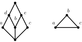
c b a
d e
c b a
Figure 2.1: The canonical join complex is an empty triangle.
possible”. This lattice also exhibits some unpleasant topological properties. We will see below that the combinatorics of the canonical join complex are closely related to the topology of its lattice.
The crosscut complex ofL is the abstract simplicial complex whose faces are the subsets A′ of atoms in L such that⋁A′<ˆ1. A lattice is crosscut-simplicial if the crosscut complex
for each interval is either a simplex or the boundary of a simplex. The Crosscut Theorem says that the order complex of a finite posetP is homotopy equivalent to its crosscut complex ([11, Theorem 10.8]). Therefore, if L is crosscut-simplicial then each interval [x, y] in L is either contractible or homotopy equivalent to a sphere with dimension two less than the number of atoms in[x, y]. (See also [47, Theorem 3.7].) In particular, µ(x, y) ∈ {−1,0,1}.
Observe that the facets of the crosscut complex for the latticeLin Figure 2.1 are{a, b}and {b, c}. Therefore, Lis not crosscut-simplicial. By contrast, Hersh and M´esz´aros recently showed that a large class of finite semidistributive lattices—including the class of finite distributive lattices, the weak order on a finite Coxeter group, and the Tamari lattice ([47, Theorems 5.1, 5.3 and 5.5])—are crosscut-simplicial. Building on their work, McConville proved that if L is semidistributive, then it is crosscut-simplicial ([57, Theorem 3.1]). When each element inLhas a canonical join representation, we prove that the converse is true.
Theorem 2.1.2. Suppose that L is a finite join-semidistributive lattice. The following are equivalent:
1. The canonical join complex of L is flag. 2. L is crosscut-simplicial.
3. L is semidistributive.
As an immediate corollary, we obtain the following topological obstruction to the flag prop-erty of the canonical join complex.
1. Each interval [x, y] in Lis either contractible or homotopy equivalent to Sd−2, wheredis
the number of atoms in [x, y];
2. The M¨obius function takes only the values {−1,0,1} on the intervals of L.
McConville showed in [57, Corollary 5.4] that if L is crosscut-simplicial then so is each of its lattice quotients. Because semidistributivity is preserved under taking sublattices and quotientswhenLis finite (see Section 2.4.1), we immediately obtain the following extension of McConville’s result for finite join-semidistributive lattices.
Corollary 2.1.4. Suppose thatLis a finite join-semidistributive lattice that is crosscut-simplicial. Then each sublattice and quotient lattice of L is also crosscut-simplicial.
Theorem 2.1.1 is surprising in part because its proof does not explicitly use the canonical meet representation of the elements in L. Instead, we make use of a local characterization of the canonical join representation in terms of cover relations, and a bijection κ from the join-irreducible to the meet-join-irreducible elements in L. As an easy consequence of this approach, we obtain the following nice result. In the statement, the canonical meet complex is the complex of subsetsA inL such that the meet⋀A is a canonical meet representation.
Corollary 2.1.5. Suppose thatLis a finite semidistributive lattice. Then the bijectionκinduces an isomorphism from the canonical join complex to the canonical meet complex of L.
Using the isomorphism from Corollary 2.1.5, one obtains an operation on the canonical join complex that generalizes the operation of rowmotion (on the set of antichains in a poset) and the operation of Kreweras complementation (on the set of noncrossing partitions). See Remark 2.3.15.
The canonical join complex was first introduced in [72], in which Reading showed that it is flag for the special case of the weak order on the symmetric group (see Example 2.2.6). Recently, canonical join representations have played a role in the study of functorially finite torsion classes for the preprojective algebra of Dynkin-type W, whenW is a simply laced Weyl group (see for example [41, 52]). In the forthcoming [9], the authors study the canonical join complex ofany
finite dimensional associative algebra Λ of finite representation type. Since the weak order on any finite Coxeter groupW and the lattice of torsion classes for Λ of finite representation type are both examples of finite semidistributive lattices (see [26, Lemma 9] and [41, Theorem 4.5]), we obtain the following two applications of Theorem 2.1.1:
Corollary 2.1.7. Suppose that Λ is an associative algebra of finite representation type, and
tors(Λ)is its lattice of torsion classes ordered by containment. Then the canonical join complex of tors(Λ) is flag.
2.2
Motivation and examples
Before we give the technical background for our main results, we describe several familiar examples in which the combinatorics of canonical join representations appear. We begin with an example from number theory and commutative algebra.
Example 2.2.1 (The divisibility poset). It is often useful to give a canonical factorization of the elements in a set of equipped with some algebraic structure. A familiar example is the primary decomposition of an ideal in a Noetherian ring. The canonical join representation is the natural lattice-theoretic analogue. Indeed, whenL is the the divisibility poset (whose elements are the positive integers ordered r ≤ s if and only if r∣s), the canonical join representation of x∈L coincides with the primary decomposition of the ideal generated byx:
x= ⋁{pd∶p is prime and pd is the largest power of pdividingx}.
Suppose that L is a finite lattice, such that each element in L admits a canonical join representation. One pleasant property of the canonical join representation (and its dual, the canonical meet representation) is that it “sees” the geometry the Hasse diagram forL. Suppose that w ∈ L has the canonical join representation ⋁A. We will shortly prove that the factors that appear in A are naturally in bijection with the elements covered by w. So, the down-degree of w is equal to the size ofA. Specifically, we will prove the following proposition. (See Lemma 2.3.3 and Proposition 2.3.4. Similar constructions appear in the literature, for example see [39, Theorem 3.5] which gives essentially the same statement for free lattices.)
Proposition 2.2.2. Suppose that ⋁A=w is a face in the canonical join complex of L. Then, for each elementythat is covered bywthere is a corresponding elementj∈Asuch thatj∨y=w, and j is the unique minimal element in L with this property. The correspondence y ↦ j is a bijection.
With this proposition in mind, we consider the class of finite distributive lattices.
A are the maximal elements of IA). Dually, we writeIA for the order ideal satisfying:A is the
set of minimal elements in P ∖IA. Observe that the order ideals covered by IA are exactly of
the formIA∖{y}=IA∖ {y}, wherey∈A. SinceIy is the smallest order ideal inJ(P) containing
y, it follows immediately from Proposition 2.2.2 that the canonical join representation ofIA is
⋃{Iy ∶y∈A}. (Dually, the canonical meet representation for the idealIA is ⋂{Iy ∶y ∈A}.) It
follows that the canonical join graph of J(P) is the incomparability graph ofP.
Comparability graphs were classified by a theorem of Gallai which we quote from [88, Theorem 2.1] below.
Theorem 2.2.4. A graphGis a comparability graph for a finite poset if and only if it does not contain as an induced subgraph any graph from [88, Table 1] or the complement of any graph appearing in [88, Table 2].
As an immediate corollary we have the following characterization of the canonical join graphs for finite distributive lattices.
Proposition 2.2.5. The graph G is the canonical join graph for a finite distributive lattice if and only if Gdoes not contain, as an induced subgraph, the complement of any graph forbidden by Theorem 2.2.4.
Example 2.2.6 (The Symmetric group and noncrossing arc diagrams). Reading gave an ex-plicit combinatorial model for the canonical join complex of the weak order on the symmetric group Sn in terms of certain noncrossing arc diagrams. A noncrossing arc diagram is a
diagram consisting of n nodes arranged vertically, together with a collection of curves called arcs that satisfy certain compatibility conditions. In particular, the arcs in a noncrossing arc diagram do not intersect in their interiors. (See [72] or Section 3.2.2 for details.) Each diagram is determined by its combinatorial data: the endpoints of its arcs and on which side (either left or right) each arc passes the nodes in the diagram.
Figure 2.2: Some examples of noncrossing arc diagrams.
of the Theorem, we take “a collection of arcs” to also mean a collection of noncrossing arc diagrams, each containing a single arc.)
Theorem 2.2.7. There is a bijection δ from the set of join-irreducible permutations in Sn to the set of noncrossing arc diagrams on n nodes that contain precisely one arc. Moreover, a collection of arcs E corresponds to a face in the canonical join complex of Sn if and only if the arcs in E are pairwise compatible.
Example 2.2.8 (The Tamari lattice and noncrossing partitions). Recall from Example 1.5.2, the Tamari lattice Tn is a finite semidistributive lattice (see for example [42, Theorem 3.5]),
which can be realized as an ordering on the set of triangulations for a fixed convex polygon P. The simple associahedron is a convex polytope, whose faces are in bijection with the collections of pairwise noncrossing diagonals of P (see [33, Figure 3.5]). The Hasse for Tn is an
orienta-tion for the one-skeleton of the associahedron. Since the number of factors in a canonical join representation (called the canonical joinands) for w∈Tn is equal to the down-degree of w, we
obtain the following result:
Proposition 2.2.9. The f-vector for the canonical join complex of the Tamari lattice Tn is equal to the theh-vector of the rankn−1 associahedron. Specifically, the number of size-k faces in the canonical join complex is equal to the Narayana number
N(n, k) = 1 n(
n k+1)(
n k).
Indeed, the canonical join representation of w ∈ Tn is essentially a noncrossing partition.
Recall that the Tamari latticeTn may be realized as the set of permutations avoiding the
312-pattern. It is a fact that a permutation avoids the 312-pattern if and only if its image under the bijectionδ (from Theorem 2.2.7) is a noncrossing arc diagram consisting of only right arcs. (Aright arc is an arc that does not pass to the left of any node. See the leftmost noncrossing diagram in Figure 2.2.) Rotating such a diagram by a quarter-turn gives the familiar represen-tation of a noncrossing partition as a bump diagram. (See [72, Example 4.5] for details, and [75, Theorem 2.7] and the discussion following [75, Proposition 8.8] for a type-free discussion.)
2.3
Finite semidistributive lattices
2.3.1 Definitions
cov↓(w) for the set {y ∈L∶w ⋅>y}. Similarly, we write cov
↑(w) for the set of upper covers of
w. Recall that wisjoin-irreducible ifw= ⋁A implies that w∈A. (In particular, the bottom element ˆ0 is not join-irreducible, because it is equal to the empty join.) Since L is finite, w is join-irreducible when cov↓(w)has exactly one element.Meet-irreducible elements satisfy the
dual condition. We write Irr(L) for the set of join-irreducible elements inL.
A join-representation⋁Aofw isirredundant if⋁A′< ⋁Afor each proper subsetA′⊂A.
Each irredundant join-representation is an antichain inL. We say that the subsetAofL join-refines a subsetB if, for each element a∈A, there exists some elementb∈B such thata≤b. Join-refinement defines a preorder on the subsets ofLthat is a partial order (corresponding to the containment of order ideals) when restricted to the set of antichains in L.
We write ijr(w) for the set of irredundant join-representations of w. The canonical join representation of w in L is the unique minimal element, in the sense of join-refinement, of ijr(w), when such an element exists. We write can(w) for the canonical join representation of w. An element j ∈ can(w) is a canonical joinand for w. If A = can(w), we say that A joins canonically, orA is a canonical join representation in L (although, more precisely, we mean that the expression ⋁A is a canonical join representation). It follows immediately from the definition that each canonical joinand ofwis join-irreducible. Moreover, the canonical join representation of each join-irreducible element j exists and is equal to {j}. The canonical meet representation of w is defined dually (when it exists).
In Figure 2.3, we give two examples in which the canonical join representation of ˆ1 does not exist. In the modular lattice on the left each pair of atoms is a lowest-possible, irredundant
e a b
d c
Figure 2.3: Two finite lattices whose top elements have no canonical join representation.
join-representation for the top element. Since there is no unique such join-representation, the canonical join representation for ˆ1 does not exist. Arguing dually, we see that the canonical meet representation for the bottom element ˆ0 does not exist either. In the lattice on right, each element has a canonical meet representation. However, botha∨dandb∨care minimal elements of ijr(ˆ1). Again, the canonical join representation of ˆ1 does not exist.
and e∨b are expressions for ˆ1, bute∨ (a∧b) is equal to e. (A similar failure is easily verified among the atoms of the modular lattice.) We will see that correcting for precisely this kind of failure of distributivity guarantees the existence of canonical join representations, when L is finite.
A lattice L is join-semidistributive ifL satisfies the following implication for every x, y and z:
Ifx∨y=x∨z, then x∨ (y∧z) =x∨y (SD∨)
L ismeet-semidistributive if it satisfies the dual condition:
Ifx∧y=x∧z, then x∧ (y∨z) =x∧y (SD∧)
A lattice is semidistributive if it is join-semidistributive and meet-semidistributive. The fol-lowing result is the finite case of [39, Theorem 2.24].
Theorem 2.3.1. Suppose that L is a finite lattice. Then L satisfies SD∨ if and only if each element in L has a canonical join representation. Dually, L satisfies SD∧ if and only if each element in L has a canonical meet representation.
Assume that L is a finite join-semidistributive lattice, and let j ∈Irr(L). We write j∗ for
the unique element covered by j, and K(j) for the set of elements a∈L such that a≥j∗ and
a/≥j. When it exists, we writeκ(j) for the unique maximal element of K(j). It is immediate thatκ(j) is meet-irreducible. Below, we quote [39, Theorem 2.56]:
Proposition 2.3.2. A finite lattice L is meet-semidistributive if and only if κ(j) exists for each join-irreducible element j in L.
Below we establish a bijection from the set cov↓(w) to can(w). A similar construction also
appears in [39, Theorem 3.5]. Suppose thatw∈L. For eachy∈cov↓(w), there is some element
j∈can(w) such that y∨j=w (because there is some elementj∈can(w) such that j /≤y). For thisj, the set can(w)join-refines{j, y}. Because can(w) is an antichain, eachj′∈can(w) ∖ {j}
satisfiesj′≤y. Therefore,j is the unique canonical joinand ofwsuch thaty∨j=w. We define a
mapη∶cov↓(w) →can(w)which sendsy to the unique canonical joinandj such thaty∨j=w.
Lemma 2.3.3. Suppose that L is a finite join-semidistributive lattice, and w ∈ L. Then the map η ∶cov↓(w) →can(w) is a bijection such that y≥ ⋁can(w) ∖ {η(y)} and y∈ K(η(y)) for each y∈cov↓(w).
Proof. Suppose there exist distinctyandy′ in cov
↓(w)satisfyingη(y) =η(y
′). Then,y∨y′=w,
and can(w) does not join-refine {y, y′} (because η(y) is below neither y nor y′). We have a
this contradiction, we conclude that η is injective. Suppose that j∈can(w). Since ⋁can(w) is irredundant,⋁(can(w)∖{j}) <w. Thus, there is somey∈cov↓(w)such thaty≥ ⋁(can(w)∖{j}).
Ify≥j theny=w, and that is absurd. We conclude thatj=η(y), and thatη is a bijection. We have already argued, in the paragraph above the statement of the proposition, that y≥ ⋁can(w) ∖ {η(y)}. To complete the proof, suppose thaty∨η(y)∗=w. Since, can(w) does
not join-refine {y, η(y)∗} (because η(y) /≤ η(y)∗ and η(y) /≤ y), we obtain a contradiction as
above. We conclude that y∨η(y)∗<w. Since y is covered by w, we have y∨η(y)∗ =y. Thus,
y∈ K(η(y)), for each y∈cov↓(w).
As a consequence of Lemma 2.3.3, we obtain a proof of Proposition 2.2.2, which we restate here with the notation from of Lemma 2.3.3.
Proposition 2.3.4. Suppose that L is a finite join-semidistributive lattice, and y is covered by w in L. Then,η(y) is the unique minimal element of L such thatη(y) ∨y=w.
Proof. Suppose that x ∈L has x∨y=w. Since can(w) join-refines {x, y} and η(y) and y are incomparable, we conclude thatη(y) ≤x.
In fact, the previous proposition characterizes of finite join-semidistributive lattices. (Similar constructions exist; for example, see the proof of [1, Theorem 3-1.4].) Because the proof is similar to the proof of Lemma 2.3.3, we leave the details to the reader.
Proposition 2.3.5. Suppose thatL is a finite lattice. The following conditions are equivalent: 1. For eachw∈Land eachy∈cov↓(w), there is a unique minimal elementη(y) ∈Lsatisfying
y∨η(y) =w.
2. L is join-semidistributive.
Suppose that L is a finite join-semidistributive lattice, j ∈ Irr(L), and F is a canonical join representation. The next lemma, in particular, implies that F ∪ {j} is a canonical join representation if and only if ⋁F∨j> ⋁F∨j∗.
Lemma 2.3.6. Suppose that L is a finite join-semidistributive lattice andj∈Irr(L). Then: 1. j is a canonical joinand of y∨j, for each y∈ K(j);
2. j is a canonical joinand of ⋁F∨j if and only if ⋁F∨j> ⋁F∨j∗, for each subsetF of
L∖ {j}.
Proof. Ify=j∗, then the first statement is obvious (because{j} is the canonical join
we have A∪A′ =can(w). Also, the set A is not empty because the join y∨j is irredundant.
We want to show that A= {j}. Since j is join-irreducible, it is enough to show that j= ⋁A. Since y≥ ⋁A′, we see that⋁A∨y=j∨y. If⋁A<j, thenj
∗∨y=j∨y, and that is impossible
because y∈ K(j). We conclude that j is a canonical joinand ofy∨j.
If ⋁F∨j > ⋁F ∨j∗, then ⋁F ∨j∗ ∈ K(j). We conclude that j is a canonical joinand of
⋁F∨j. The remaining direction of the second item is straightforward to verify.
We close this subsection by quoting the following easy proposition (for example see [72, Proposition 2.2]), which says that the canonical join complex is indeed a simplicial complex. Proposition 2.3.7. Suppose L is a finite lattice, and the join ⋁A is a canonical join repre-sentation in L. Then each proper subset of A also joins canonically.
2.3.2 The flag property
In this section we prove Theorem 2.1.1. We begin by presenting the key arguments in one direction the proof: If L is a finite semidistributive lattice, then its canonical join complex is flag. Most of the work is done in the following two lemmas.
Lemma 2.3.8. Suppose that L is a finite semidistributive lattice, and F is a subset of Irr(L)
such that ∣F∣ ≥3 and each proper subset ofF is a face in the canonical join complex. Then the joins ⋁(F∖ {j}) and ⋁(F∖ {j′}) are incomparable for each distinct j and j′ in F.
Proof. Without loss of generality we assume that⋁F =ˆ1. Suppose there exists distinctj, j′∈F
such that ⋁(F∖ {j}) ≥ ⋁(F∖ {j′}). On the one hand, we have (⋁(F∖ {j})) ∨ (⋁(F∖ {j′}))
is equal to ⋁F = ˆ1. On the other hand, (⋁(F∖ {j})) ∨ (⋁(F∖ {j′})) = ⋁(F ∖ {j}). Thus,
⋁(F∖{j}) =ˆ1. SinceF has at least three elements, there existsj′′∈F∖{j, j′}. We writew′for
j j∗ ⋁F∖ {j, j′}
⋁F∖ {j, j′′}
w′
w′′ ⋁F∖ {j} =ˆ1
y′
y′′
Figure 2.4: Dashed lines represent order relations inLwhile solid lines represent cover relations.
faces in the canonical join complex,j is a canonical joinand for both w′ and w′′. Lemma 2.3.3
implies that there exists y′ ∈ cov ↓(w
′) and y′′ ∈ cov ↓(w
′′) such that y′, y′′ ∈ K(j). Moreover,
y′≥ ⋁(F∖ {j, j′}) and similarly y′′≥ ⋁(F∖ {j, j′′}).
So, we have:y′∨y′′≥ (⋁(F∖ {j, j′}))∨(⋁(F∖ {j, j′′})) = ⋁(F∖{j}). Since⋁(F∖{j}) =ˆ1,
we conclude that ⋁ K(j) =ˆ1, contradicting Proposition 2.3.2.
Lemma 2.3.9. Suppose that L is a finite join-semidistributive lattice, and F is a subset of
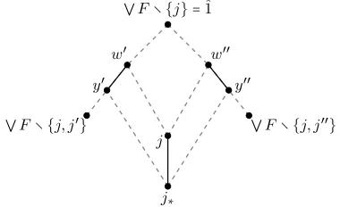
Irr(L) satisfying the following conditions: First, ∣F∣ ≥3; second, each proper subset of F is a face in the canonical join complex of L; third,⋁F is irredundant; fourth F is not a face of the canonical join complex. Then there exists j∈F such that κ(j) does not exist.
Proof. Without loss of generality, we assume that ⋁F =ˆ1. Since the join ⋁F is irredundant, there exists somej∈F such thatj/∈can(ˆ1). Lemma 2.3.6 implies that⋁(F∖{j})∨j∗=ˆ1. Letj
′
andj′′be distinct elements inF∖{j}. As in the proof of Lemma 2.3.8, lety′andy′′be the unique
elements covered by⋁F∖{j′}and⋁F∖{j′′}, respectively, withy′, y′′∈ K(j). Thus,y′, y′′≥j ∗.
Also y′≥ ⋁(F∖ {j, j′}) and y′′≥ ⋁(F∖ {j, j′′}). Therefore, y′∨y′′≥ ⋁(F∖ {j}) ∨j
∗=ˆ1. The
statement follows.
Proof of one direction of Theorem 2.1.1. We show that ifLis semidistributive, then its canon-ical join complex is flag. Suppose that F ⊂ Irr(L) such that ∣F∣ ≥ 3 and each proper subset of F is a face of the canonical join complex. Without loss of generality, assume that ⋁F =ˆ1. Lemma 2.3.8 says that for each distinct j and j′ inF, the joins ⋁(F∖ {j}) and ⋁(F ∖ {j′})
are incomparable. Thus, we have
⋁(F∖ {j}) < (⋁(F∖ {j})) ∨ (⋁(F∖ {j′
})) = ⋁F.
We conclude that ⋁F is irredundant. Lemma 2.3.9 implies that F is a face of the canonical join complex.
We now turn to the other direction of Theorem 2.1.1. In the following lemmas we will assume thatL is a finite join-semidistributive lattice in which failsSD∧. By Proposition 2.3.2, there is
some j ∈Irr(L) such that κ(j) does not exist. Our goal is to construct a set A ⊂Irr(L) such that A∪ {j} is a “hollow face” in the canonical join complex. More precisely, the set A must satisfy the following conditions. (NF stands for “not-flag”.)
(NF1) A∪ {j} isnot a face in the canonical join complex of L.
(NF2) Each pair of elements inA∪ {j} is a face in the canonical join complex.
to be minimal in join-refinement. The argument is somewhat delicate because join-refinement is a preorder, not a partial order, on subsets of L. So, we must take extra care to compare only antichains Y ⊂Irr(L) satisfying (NF1). To further emphasize this point, we write A≪B when A join-refinesB, forantichains A and B. We writeA(j) for the collection of antichains Y ⊆L∖ {j} satisfying Y ∪ {j} is an antichain. We write E(j) for the set of j′ ∈Irr(L) ∖ {j}
such thatj′∨jis a canonical join representation. When it is possible, we suppressj, and simply
write E.
Lemma 2.3.10. Suppose that L is a finite join-semidistributive lattice and j ∈ Irr(L) such thatκ(j) does not exist. LetE be the set ofj′∈Irr(L) ∖ {j}
such thatj′∨
j is a canonical join representation. Then:
1. ⋁E∨j= ⋁E∨j∗;
2. There exists a nonempty antichain Y in A(j) such that ⋁Y ∨j= ⋁Y ∨j∗.
Proof. Assume that⋁E∨j> ⋁E∨j∗. Lemma 2.3.6 says thatjis a canonical joinand of⋁E∨j.
Also, for each elementainK(j),jis a canonical joinand ofa∨j. That is,a∨jhas the canonical join representation ⋁E′∨j for some subset E′ ⊂ E. Thus a∨j ≤ ⋁E∨j, and in particular
a≤ ⋁E∨j. Lemma 2.3.3 implies that there is a unique elementy ∈ K(j) covered by⋁E∨j. If a /≤y, then y∨a= ⋁E∨j. Proposition 2.3.4 says that j is the unique minimal element of L whose join withy is equal to ⋁E∨j. Therefore, j≤a, contradicting the fact thata∈ K(j). We conclude that a≤ y. We have proved that y = κ(j), contradicting our hypothesis. Thus, ⋁E∨j= ⋁E∨j∗.
For the second statement, observe that if E is empty, then Lemma 2.3.6 implies that K(j) = {j∗}, contradicting the assumption that κ(j) does not exist. We conclude that E
is nonempty. Since the antichain of maximal elements Y ⊆E satisfies ⋁Y = ⋁E, we have the desired result.
Lemma 2.3.10 says that the collection of antichains Y inA(j) satisfying
⋁Y ∨j= ⋁Y ∨j∗ (N C)
is nonempty. (Actually, we have shown something stronger: The collection of antichainsY ⊆ E(j) that satisfy (N C) is nonemtpy.) We write (N C) for “not-canonical” because Lemma 2.3.6 im-plies that ⋁Y ∨j is not a canonical join representation. In particular, j is not a canonical joinand of⋁Y ∨j.
join complex for eachb∈B. Thus, ifB has at least three elements, thenB∪ {j} is the “hollow face” that we want to construct. We will deal with the case where∣B∣ ≤2 in Lemma 2.3.12 and Lemma 2.3.13.
Lemma 2.3.11. Suppose that L is a finite join-semidistributive lattice and j ∈ Irr(L) such thatκ(j) does not exist. Among all antichains inA(j) that satisfy (N C), letB be minimal in join-refinement. Then (B∖ {b}) ∪ {j} is a canonical join representation, for eachb∈B. Proof. We begin by pointing out two easy observations about the join-refinement relation. (Note that the second observation, (JR2), may fail if S∪ {x} and T∪ {x} are not antichains.) (JR1) For any pair of subsets S and T, if S join-refines T then each subset S′ ⊆ S also
join-refinesT.
(JR2) Suppose that S∪ {x} and T ∪ {x} are antichains. Then, S∪ {x} ≪T ∪ {x} if and only ifS≪T.
In particular, (JR1) implies that B ∖ {b} ≪B. Thus, ⋁ (B∖ {b}) ∨j∗ < ⋁ (B∖ {b}) ∨ j.
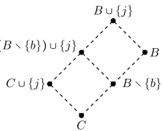
Lemma 2.3.6 says that j is a canonical joinand of ⋁ (B∖ {b}) ∨j. We write C∪j for the canonical join representation of ⋁ (B∖ {b}) ∨j, where j ∉C. We claim that C∪ {b} = B. In Figure 2.5, we depict the relationship betweenC,B, andB∖{b}in the join-refinement order. In the figure, we haveC∪{j} ≪ (B∖{b})∪{j}, becauseC∪{j}is the canonical join representation for⋁(B∖ {b}) ∨j. By (JR2), we have C≪B∖ {b}.
C
B∖ {b} C∪ {j}
(B∖ {b}) ∪ {j}
B B∪ {j}
Figure 2.5: Some order relations in the join-refinement order forL.
We make two observations that follow immediately from Lemma 2.3.6. First, we observe thatj not a canonical joinand of⋁B∨j. Thus,
⋁C∨j= ⋁(B∖ {b}) ∨j< ⋁B∨j. (2.3.1)
Second, we observe that:
Indeed, if⋁ (C∪ {b})∨j∗< ⋁ (C∪ {b})∨j then Lemma 2.3.6 says thatj is a canonical joinand
of⋁ (C∪ {b}) ∨j= ⋁B∨j. We have just noted thatj is a not a canonical joinand for ⋁B∨j. If C∪ {b} is an antichain, then applying (JR2) to the relation C≪B∖ {b}, we have C∪ {b} ≪B. Thus, we have C∪ {b} is an antichain inA(j) that satisfies (N C) and join-refines B. By minimality ofB, we conclude thatC∪ {b} =B as desired. So, we assume thatC∪ {b}is not an antichain. The inequality in (2.3.1) implies that there exists noc∈C withb≤c. We write C′
for the set {c∈C∶ c<b}.
C
B∖ {b} C∪ {j}
(B∖ {b}) ∪ {j} B B∪ {j}
C∖C′
(C∖C′) ∪ {
b}
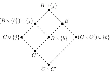
Figure 2.6: Some relations in the join-refinement order forL.
We make three easy observations: First, (C∖C′) ∪ {b} is member of A(j). Second,
apply-ing (JR1) to the relation C≪B∖ {b}, we have that C∖C′≪B∖ {b}. By (JR2), we conclude
that(C∖C′) ∪ {b} ≪B. We depict these relations in Figure 2.6. Third,
⋁((C∖C′) ∪ {
b}) ∨j= ⋁(C∪ {b}) ∨j= ⋁(C∪ {b}) ∨j∗= ⋁((C∖C ′) ∪ {
b}) ∨j∗,
where the first and third equalities follow from the fact that⋁(C∪{b})is equal to⋁(C∖C′)∪{b},
and the middle equality is (2.3.2).
Therefore, the set(C∖C′)∪{b}is an antichain inA(j)that satisfies (N C) and join-refinesB.
By the minimality of B, we have B = (C∖C′) ∪ {b}. SinceC≪B∖ {b}, we have that C
join-refines its proper subset C∖C′. That is a contradiction (becauseC is an antichain). Thus, C′
is empty. We have proved the desired result.
Our candidate for a “hollow face” in the canonical join complex is the antichainB∪{j}from Lemma 2.3.11. As we have noted, ifB has at least three elements then B satisfies both (NF1) and (NF2).
Suppose that B = {b1, b2}. By Lemma 2.3.11, {j, bi} is a canonical join representation, for
Lemma 2.3.12. Suppose that Lis a finite join-semidistributive lattice andj∈Irr(L) such that
κ(j) does not exist. Among all antichains inA(j) that satisfy (N C), let B be minimal in join-refinement. Suppose that B has at least two elements. Then each pair of elements inB∪ {j}is a face in the canonical join complex.
Proof. If B has three or more elements, then the statement follows from Lemma 2.3.11 and Proposition 3.2.1. Assume that B has two elements, b1 and b2. By Lemma 2.3.11, we have
{j, bi} is a canonical join representation, fori=1,2. Consider{b1, b2}. We will argue thatb1 is
a canonical joinand of b1∨b2, and complete the proof by symmetry.
Assume that (b1)∗∨b2=b1∨b2. We observe that (b1)∗∨b2∨j= (b1)∗∨b2∨j∗. If(b1)∗≤j∗,
then we have b2∨j = b2∨j∗, contradicting Lemma 2.3.6. By the same reasoning, (b1)∗ /≤b2.
Also, j /≤ (b1)∗ because b1 and j are incomparable. Similarly, b2 /< (b1)∗. Thus, {(b1)∗, b2}
is an antichain in A(j) that satisfies (N C) and join-refines {b1, b2}. But this contradicts our
hypothesis, which says thatB is minimal in join-refinement among all such antichains. By this contradiction, we conclude that (b1)∗∨b2 < b1∨b2. Lemma 2.3.6 says that b1 is a canonical
joinand ofb1∨b2.
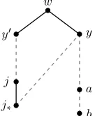
Finally, we turn to the case where B is a singleton. This turns out to be a non-issue. The next lemma says that we can always find such an antichain inA(j)with at least two elements. Lemma 2.3.13. Suppose that Lis a finite join-semidistributive lattice andj∈Irr(L) such that
κ(j) does not exist. Then there exists an antichainA∈A(j) satisfying: 1. A has at least two elements; and
2. A is minimal in join-refinement among all antichains in A(j) that satisfy (N C).
Proof. Recall that E(j) is the set of j′ ∈ Irr(L) ∖ {j} such that j′∨j is a canonical join
representation. Take A to be a nonempty antichain that is minimal in join-refinement among all antichains Y ⊆ E(j) that satisfy (N C). Lemma 2.3.10 implies that such an antichain A exists. For each a∈A, we have a∨j is a canonical join representation. It follows immediately from Lemma 2.3.6 that Ahas at least two elements.
b a y
j∗
j y′
w
Figure 2.7: A depiction of the argument for Lemma 2.3.13. Dashed lines represent order rela-tions inL while solid lines represent cover relations.
Write wfora∨j. Since a∨jis the canonical join representation ofw, Lemma 2.3.3 implies that cov↓(w) has precisely two elements,y and y
′. Let η(y) =j and η(y′) =a, so thaty∈ K(j)
andy≥a. See Figure 2.7. Thus, we haveb≤a≤y. On the one hand,(b∨j) ∨y= (b∨j∗) ∨y=y.
On the other hand,b∨ (j∨y) =b∨w=w. By this contradiction, we have proved the result. Finally, we complete the proof of the main result.
Proof of the remaining direction of Theorem 2.1.1. Now we argue that if L is a finite join-semidistributive lattice and the canonical join complex of L is flag, thenL is semidistributive. By Proposition 2.3.2, it is enough to show that for eachj∈Irr(L) the element κ(j) exists.
Suppose j ∈Irr(L) and κ(j) does not exist. Among all nonempty antichains inA(j) that satisfy (N C), let A be minimal in join-refinement, and choose A so that it has at least two elements. Lemma 2.3.13 says that such an antichainAexists. Lemma 2.3.6 implies thatA∪ {j} is not face of the canonical join complex. Finally, Lemma 2.3.12 says that each pair of elements in A∪ {j} is face in the canonical join complex. We have reached a contradiction to our hy-pothesis that the canonical join complex is flag. By this contradiction, we conclude that L is semidistributive.
Suppose thatm is meet-irreducible and writem∗ for the unique element coveringm. When
it exists, letκ∗(m) be the smallest element j∈Lwith j≤m∗ and j /≤m. It is immediate that
κ∗(m) is join-irreducible. Proposition 2.3.2, applied to the dual lattice, says that L is
meet-semidistributive if and only if κ∗(m) exists for each meet-irreducible element m. In fact, L is
semidistributive if and only ifκ is a bijection, with inverse mapκ∗; this is the finite case of [39,
Corollary 2.55]. Applying the dual argument for the canonical meet complex, we immediately obtain the following result. (Recall that Theorem 2.3.1 says that each element in L has a canonical meet representation if and only if Lis meet-semidistributive.)
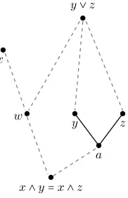
Next, we prove Corollary 2.1.5 by showing that the bijection κ taking a join-irreducible elementjtoκ(j)induces an isomorphism from the canonical join complex ofLto the canonical meet complex of L.
Proof of Corollary 2.1.5. Corollary 2.3.14 says that the canonical meet complex of L is flag, so it is enough to show that κ bijectively maps edges of the canonical join complex to edges of the canonical meet complex. Suppose that {j1, j2} is a face of the canonical join complex,
and write m1 for κ(j1) and m2 for κ(j2). Suppose that m1∧m2 = (m1)∗∧m2. Lemma 2.3.3
implies that there exists some y ∈ cov↓(j1 ∨j2) satisfying : j1 ≤ y ≤ κ(j2). (See Figure 2.8
for an illustration.) Since j1 ≤ (m1)∗, we conclude that j1 ≤ (m1)∗∧m2 = m1 ∧m2. We see
that j1 ≤ m1 and that is a contradiction. Therefore, (m1)∗ ∧m2 > m1 ∧m2. By the dual
statement of Lemma 2.3.6, we conclude that m1 is a canonical meetand of m1∧m2, and by
symmetrym2is also a canonical meetand ofm1∧m2. The dual argument establishes the desired
isomorphism.
y j1∨j2
j1
(j1)∗ (m1)∗
κ(j1) =m1 j2
(j2)∗
Figure 2.8: An illustration of the argument for the proof of Corollary 2.1.5. Dashed gray lines represent relations inL while solid black lines represent cover relations.
We close this section by relating Corollary 2.1.5 to Example 2.2.3 and Example 2.2.8, from Section 2.2.
Remark 2.3.15. Suppose that F is a face of the canonical join complex of a finite semidis-tributive lattice L. Corollary 2.1.5 says that ⋀κ(F) is a canonical meet representation. By taking the canonical join representation of ⋀κ(F), we can view the map κ as an operation on the canonical join complex. Similarly, we can view κ∗ as an operation on the canonical meet
complex.
partitions (that is, the set of antichains in the root poset for a finite cystrallographic root system) coincide. Indeed, both maps are an instance of the operation ofκ (orκ∗) on the canonical join
complex (or canonical meet complex).
On the one hand, the action ofκon the canonical join complex of the Tamari lattice coincides with Kreweras complementation (recall from Example 2.2.8 that canonical join representations in the Tamari lattice are essentially noncrossing partitions). On the other hand, Panyshev complementation is a special case of an operation on the set of antichains in a finite poset P calledrowmotion, as we now explain. WhenA is an antichain inP, we write Row(A) for the antichain {x∈ P ∶x is minimal among elements not in IA}. (Our notation is based on [86]. See
also [3, 18, 19, 37, 62, 80].) So, we haveIA=IRow(A). It follows immediately from the definition
of κ∗ that κ∗(I y) ↦I
y. We obtain the following result.
Proposition 2.3.16. Suppose that P is a finite poset, and A is an antichain in P. Then the map κ∗, acting on faces of the canonical meet complex ofJ(P), sends the order ideal I
Ato the order ideal IRow(A).
2.3.3 Crosscut-simplicial lattices
In this section, we prove Corollary 2.1.2. Recall that one direction of the proof was given as [57, Theorem 3.1]. Because it is easy, we give an alternative argument in the next paragraph.
Write A for the set of atoms in L. When L is a finite semidistributive lattice every join of two atoms is a canonical join representation. In particular, Theorem 2.1.1 implies that each distinct subset of atoms gives rise to a distinct element inL. Thus the crosscut complex for L is either the boundary of the simplex onAor equal to the simplex onA, depending on whether ⋁A = ˆ1 or ⋁A < ˆ1. Since each interval in L inherits semidistributivity, it follows that L is crosscut-simplicial.
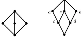
Figure 2.9: A finite crosscut-simplicial lattice failing both SD∨ and SD∧.
shown in Figure 2.9. This lattice fails both SD∨ and SD∧.) Join-semidistributivity gives us a
powerful restriction: A finite join-semidistributive latticeL fails SD∧ if and only if Lcontains
the lattice shown in Figure 2.1 as a sublattice ([39, Theorem 5.56]).
We now begin our proof. The following lemmas will be useful. The first lemma is a local version of Theorem 2.3.1, and appears as [73, Lemma 9-2.5].
Lemma 2.3.17. Suppose thatL is a finite lattice satisfying the following property:
If x, y, and z are elements of L with x∧y = x∧z and also, y and z cover a common element, then x∧ (y∨z) =x∧y.
Then L is meet-semidistributive.
Lemma 2.3.18. Suppose that L is a finite join-semidistributive lattice that fails SD∧. Then there exists x, y, and z such that y∨z>x and x, y, and z cover a common element.
Proof. We prove the proposition by induction on the size ofL. As mentioned above,Lcontains the lattice shown in Figure 2.1 as sublattice, and this proves the base case. By Lemma 2.3.17, we can assume that there exist x, y, and z in L such that x∧y =x∧z, x∧ (y∨z) ≠ x∧y, and cov↓(y) ∩cov↓(z)is not empty. Among all such triples, we choose{x, y, z}minimal in
join-refinement. Write a for the element in cov↓(y) ∩cov↓(z) (if there is more than one element in
cov↓(y) ∩cov↓(z), theny∧z does not exist). If x also covers a, then we are done (because if
x ⋅>aand y∨z/>x, then(y∨z) ∧x=a, and that contradicts our assumption that{x, y, z} fail SD∧). So we assume thatx does not covera.
x
y∨z
w
y z a x∧y=x∧z
Figure 2.10: Dashed lines represent relations inL and solid lines represent cover relations.