Support for Virtualization in Data Centers.

Abstract

AMBADKAR, ADITYA RADHAKRISHNA. Support for Virtualization in Data Centers. (Under the direction of Dr. Yannis Viniotis.)

Modern data centers largely depend of virtualization. It has presented engineers with lot of opportunities to innovate.

I would not be exaggerating in saying, live virtual machine (VM) migration was a killer app for virtualization. Due to its numerous benefits pertaining to ease of management of servers, power, policies etc. it soon became one of the most used features in virtual data centres. The flip side of the coin is, right from the beginning live VM migration has been a challenge to network designers and administrators. They need to account for the migration domain, VM state, downtime and what not to support it. The center point of these problems is maintaining the external state associated to the VM such as the live TCP connections, firewall policies, VLAN information etc. after the VM migrates to its destination. Several solutions have been proposed to solve this problem but, they are either restrictive in allowed domain of the migration or they have architectural restrictions where user has to design the data center ground up to apply them.

We solved this problem from a different perspective. The desired outcome of this work was designer should not be required to change their network architecture or build their data center ground up just to accommodate a solution that solves part of all the challenges that data center have to face. We wanted a solution that could be easily integrated in running data centers and to our surprise we found the solution that is simple and easy to scale to large data centers.

©Copyright 2013 by Aditya Radhakrishna Ambadkar

Support for Virtualization in Data Centers

by

Aditya Radhakrishna Ambadkar

A thesis submitted to the Graduate Faculty of North Carolina State University

in partial fulfillment of the requirements for the Degree of

Master of Science

Computer Networking

Raleigh, North Carolina

2013

APPROVED BY:

Dr. Mihail L. Sichitiu Dr. Michael Devetsikiotis

Dedication

Biography

Aditya was born in the city of black gold (coal), Chandrapur, in state of Maharashtra in India. He is the youngest of Ujwala and Radhakrishna Ambadkar’s children.

Aditya finished his schooling and undergraduate education from his home town, Aurangabad. He was actively involved in study of robotics during his undergraduate days and application of various algorithms developed for networks triggered his interest in study of computer network-ing. During undergraduate years, he studied programming, computer networking and network security that gave him solid foundation in the field.

After graduation, he choose to work for a small company over a lucrative offer from a multi-national corporation. This gave him higher responsibilities and presented more opportunities to learn. Impressed by his domain knowledge, the management moved him to the position of contractor for Cisco Systems. In his work with Cisco, he was got the opportunity to delve deeper in the world of virtualization and data centres. He was fascinated by the challenges the field presented and decided to pursue further education in this domain.

He chose Computer Networking at North Carolina State University because of the breadth and depth of courses that it offers in the domain. At NC State, Aditya worked on projects involving enterprise network design, Software Defined Networks (Cisco onePK), survivability of data centers, behavior of TCP in virtual data center environments etc. He has also contributed to open source community via Wireshark.

Looking at his area of interest, Dr. Viniotis accepted him as his research student leading to the work presented in this report.

Acknowledgements

I would like to thank my parents for the sacrifices they have made for me to be able to complete my graduate education.

I would like to thank my Gurus Dr. Viniotis, Param Pujya Shri Pund Kaka, Param Pujya Shri Narayan Kaka Dhekne Maharaj and Dr. Mukundraj Maharaj. They have made sure that I am always focused on my goals. Their support has not only been in the form of knowledge but also to keep my soul at peace through the ups and downs of life. Their guidance and support has always been a constant and profound influence.

My sisters Mukta, Anupama and Amruta and my brother Abhijit have played a crucial role in keeping me sane all this while.

Table of Contents

List of Figures . . . vi

Chapter 1 Introduction . . . 1

1.1 Data Centres . . . 1

1.1.1 History . . . 1

1.1.2 Different topologies, their requirements and benefits . . . 2

1.2 Problem Definition . . . 7

1.2.1 Migration of services . . . 7

1.2.2 Failures . . . 8

1.3 Solution Characteristics . . . 9

1.3.1 Zero downtime . . . 9

1.3.2 Management traffic overhead due to broadcasts . . . 9

1.3.3 Service Level Agreements . . . 9

1.4 Related Work . . . 10

1.5 Implementation Overview . . . 11

1.5.1 Software Defined Networking . . . 11

1.5.2 Cisco ONE Platform Kit (onePK) API . . . 12

Chapter 2 Algorithm Design . . . 13

2.1 Problem Definition . . . 13

2.2 Algorithm Definition . . . 17

2.2.1 Pseudocodes . . . 17

2.2.2 Validation Procedure . . . 26

2.2.3 Validation . . . 27

2.3 Discussion . . . 37

Chapter 3 Implementation and Verification . . . 40

3.1 Implementation Overview . . . 40

3.2 Testbed Details . . . 42

3.3 Verification . . . 43

3.3.1 Experiment I . . . 43

3.3.2 Experiment II . . . 44

3.3.3 Experiment III . . . 47

Chapter 4 Future Work and Conclusion . . . 49

List of Figures

Figure 1.1 Hierarchical Network Design Reference Model [1] . . . 3

Figure 1.2 Two most popular trees used in data center architectures . . . 6

Figure 1.3 How software interacts with networks today . . . 11

Figure 1.4 How software interacts with networks with onePK . . . 12

Figure 2.1 Path from core switch to access switch connected to initial placement . . 14

Figure 2.2 Path from core switch to access switch connected to final placement . . . 14

Figure 2.3 DC-Tree of height four . . . 15

Figure 2.4 DC-Tree with affected elements . . . 17

Figure 2.5 Fat tree module used for asymptotic analysis . . . 19

Figure 2.6 Three possible reductions of Fat tree . . . 28

Figure 2.7 Proof of reduction of all possible placements ofSi and Sf to three cases . 29 Figure 2.8 DC-Tree made from Clos topology . . . 37

Figure 2.9 Representation of abstract node on aggregation level . . . 38

Figure 3.1 Network topology used for Experiments . . . 43

Figure 3.2 Comparison of linear growth rate with actual growth rate with respect to number of affected elements due to the migration . . . 46

Chapter 1

Introduction

1.1

Data Centres

There is no single definition of a data center. For the purpose of this report, we define a data center as a collection of compute devices that provide services.

As we have a collection of devices working together; an obvious requirement to build a data center is providing ability to the distributed compute to communicate as effectively as possible. Supporting this requirement is easier said than done. For decades, designers and managers of these networks have struggled to build such networks. This has lead to lot of research in this area.

1.1.1 History

If we consider the concept of having lot of compute power which is co-located, we can guess that information technology industry stated with this idea in form of Mainframes. One of the first such attempts was ENIAC developed by US Army in 1960’s. ENIAC was released in the pre-microprocessor era and could perform about 5000 operations per second. Intel released first commercial microprocessor in 1970’s. We can see more data centres were built for businesses in this period. We also see efforts towards disaster recovery during this period but the advancement of PCs lead to decrease in popularity of Mainframes [4].

There was a boom in PC industry during 1980’s and one of the most important realizations was need of management of IT infrastructure. Companies started consolidating servers in ded-icated rooms around 1990’s but data centres had to wait for the dot-com boom to regain their popularity. Companies built data centres to aid both system development and operations. Lot of large corporations like Rackspace started their business during the dot-com boom era [4].

corporations are running their businesses using data centres and at the same time leveraging them to deliver services to their customers. This popularity of data centres is a result of the fact that todays data centres have tremendous compute and storage capacity, they are highly reliable (tier four data centres have more than 99.995% uptime which means less than 30 mins downtime per year), they are efficient and easy to manage. One of the major technology that led to such data centres is virtualization. Almost all of the data centres today use virtualization in some form.

One of the recent trends due to such growth in virtual data centres is provision of virtual services. A virtual service is a service that is delivered via abstract ( typically virtual ) in-frastructure hence making it scalable on demand, optimized for such virtual delivery but the receiving end never realizes any difference.

We have made an attempt to support virtualization of services in data centres in this report. We want to make support for virtualization in data centres seamless and provide solutions that can be readily integrated in not only the newly built data centres but also the existing one’s without significant changes.

1.1.2 Different topologies, their requirements and benefits

Lot of different designs have been proposed over decades for data center fabrics [26, 24, 12, 14, 30]. Following is a brief discussion on some of the most popular research and industry works in the area.

A. Cisco Data center 3.0:

Today, the most popular data center architecture is a tiered structure. Cisco Systems released the following as their Data Centres 3.0 architecture in July 2011 [1]. It is built on the concept of investment protection, allowing incremental integration of new technolo-gies and platforms into the existing infrastructure to meet changing business needs. The architecture is based on a solid hierarchical foundation providing high availability and continued scalability. It constructs the network in to a three layered hierarchy consisting of access, aggregation and core layers.

for availability and performance. Hierarchical network design has been commonly used in

Figure 1.1: Hierarchical Network Design Reference Model [1]

enterprise networking for many years. This model uses redundant switches at each layer of the network topology for device-level failover that creates a highly available transport between end nodes using the network. Data center networks often require additional ser-vices beyond basic packet forwarding, such as server load balancing, firewall, or intrusion prevention. These services might be introduced as modules populating a slot of one of the switching nodes in the network, or as standalone appliance devices. Each of these service approaches also supports the deployment of redundant hardware to preserve the high availability standards set by the network topology.

A structured data center environment uses a physical layout that correlates tightly to the hierarchy of the network topology. Careful planning in conjunction with networking requirements and an eye toward flexibility for the future is critical when designing the physical data center environment is important. Taking a modular approach to data center design provides flexibility and scalability in both network topology design and utilization of physical resources.

B. DCell:

incremental expansion. Second, data center network (DCN) must be fault tolerant against various types of server failures, link outages, or server-rack failures. Third, DCN must be able to provide high network capacity to better support bandwidth-hungry services.

DCell uses a recursively defined structure to interconnect servers. High level DCells are recursively built using low level DCells forming a fully connected graph. DCell architec-ture addresses various failures at link, server and server-rack levels - by its rich physical connectivity and distributed fault tolerant routing protocol.

Using experimental results authors proved that DCell is resilient to both link and node failures. Also, the paper shows that DCell detects link failures much faster than node failures. Paper also shows that DCell achieves higher throughput than tree based schemes. It achieves scale, fault-tolerance, high network capacity and incremental expansion.

C. PortLand:

PortLand [26] is a scalable and fault-tolerant layer 2 data center network fabric. It uses a location based soft state of a pseudo-mac (PMAC) address to achieve routing at layer 2.

Mysore et. al. define an algorithm to dynamically find node’s PMAC and maintain the PMAC to actual MAC (AMAC) mapping in a centralized fabric manager. The PMAC calculation algorithm runs a Location Discovery Protocol (LDP) which is also defined in the paper. PortLand relies on its routing protocol for fault tolerance. It uses keep alive messages of LDP to detect a link or node failure. Upon not receiving a keepalive for a configurable period of time, a node assumes a link failure. Fault correction is done with following steps: (1) The detecting node informs the fabric manager about the failure (2) The fabric manager maintains a logical fault matrix with per-link connectivity infor-mation for the entire topology and updates it with the new inforinfor-mation (3) The fabric manager informs all affected switches of the failure, which then individually recalculate their forwarding tables based on the new version of the topology.

Traditional routing protocols require all-to-all communication among n nodes withO(n2) network messages and associated processing overhead. PortLand requiresO(n) communi-cation and processing, one message from the switch detecting failure to the fabric manager and, in the worst case,nmessages from the fabric manager to affected nodes.

D. VL2:

VL2’s design explores a new split in the responsibilities between host and network using a layer 2.5 shim in server’s network stack to work around limitations of the network devices. It uses Valiant Load Balancing (VLB) to spread traffic across all available paths without any centralized coordination or traffic engineering. Using VLB, each server independently picks a path at random through the network for each of the flows it sends to other servers in the data center.

Authors performed a stressed performance test on VL2 and it was found that the combi-nation of Clos with VLB gives acceptable performance in the network. The convergence was tested with all-to-all data shuffle along with disconnection of links between interme-diate and aggregation switches until only one intermeinterme-diate switch remains connected and the removal of one additional link would partition the network. It was seen that even under such severe failures, network converged in less than one sec time.

E. Applying NOX to data centres:

NOX is a piece of the Software Defined Networking ecosystem. It is specifically, a plat-form for building network control applications [27]. We have already discussed two network topologies PortLand and VL2. Both have a centralized component to handle address map-pings. VL2 and PortLand provide a small set of logically centralized primitives whereas, NOX provides a logically centralized programming environment with a powerful set of abstractions [13].

A NOX-managed network consists of one or more controllers running NOX and a set of controllable switches. The controllable switches allow NOX to specify flow entries in their forwarding table. These flow entries are of the form< header;action >, where the second item describes the action that should be applied to any packet that matches the header fields listed in the first item. Commonly used actions include: forward to port x, forward to a controller, drop, and forward to port x with the following header fields rewritten with y.

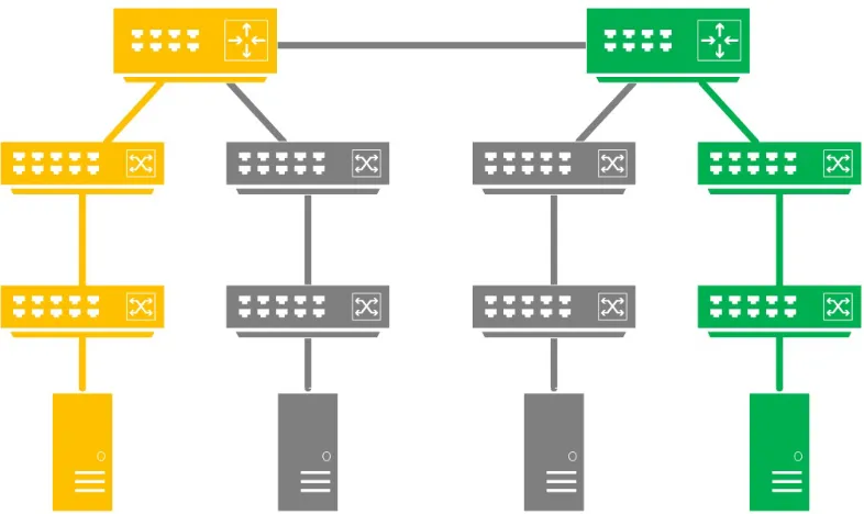
Most of these architectures are based off two basic tree structures: Fat tree [21] show in Figure 1.2a and Clos [10], [8] shown in Figure 1.2b.For the purposes of this report we are focusing only on fat trees.

(a) Fat tree k=3

(b) CLOS

Figure 1.2: Two most popular trees used in data center architectures

Another strength of fat trees is that they are modular in nature. Modularity helps scalability in data centres as we can easily add new modules to the existing infrastructure thus adding capacity. This property was so important that three giants in the field of data center infras-tructure viz. VMWare Inc., Cisco Systems and EMC Corporation came together and formed a company VCE (www.vce.com) in late 2009 to manufacture modules of data center. They intend their customers to directly use to these modules to scale their data centers thus saving time and increasing reliability.

Fat tree is a special case of Clos tree. Clos tree defines an identical entry and exit circuit and series of interconnecting circuits that are again identical. Mapping to Figure 1.2b stage 1 can be the entry circuit, stage 3 the exit circuit and stage 2 the internal circuit.

1.2

Problem Definition

In this section we discuss problems in contemporary virtual data centres that motivated us to do this work. Specific problem that we have solved has been defined in section 2.1.

1.2.1 Migration of services

Data centres today provide various services. Some of the examples of such services can be email service provided by say Gmail or Microsoft Exchange which are deployed in data centres, video on demand service provided by companies like Netflix through Amazon’s AWS cloud data centres, Xbox 360 and Sony Playstation network etc.

The most popular way to deploy services is to deploy them as services running on virtual machines. Virtual machines are quickly replacing bare metal servers as platform to run services. Virtualization enables hardware and CPU sharing between multiple virtual machines (VMs) i.e. user can run multiple VMs on the same physical host. There is complete isolation provided be-tween different VMs. This provides several advantages such as maximum utilization of resources like CPU, memory etc., exploiting and sharing resource pools, reducing the number of physical servers required, ease of management, effective power management etc.

One of the most important feature of virtualization is live migration of VMs. In live VM migration, a running VM migrates from one physical host to other. The key of live VM migration (which added live to the name) is that the all the parties involved in migration should not realize that anything changed [25], the only change that is noticeable is the slight downtime when the VM stops on source and starts on destination. Lot of commercial solutions like VMWare vMotion, Citrix XenMotion etc. have been developed which address live VM migration.

migration. Some of the challenges for the infrastructure to support the change are as follows —

• Maintain IP address of the VM so as to maintain TCP connections

• Maintain network state associated to the VM: VLAN information, ACLs, firewall rules etc.

• Change forwarding information in the network to avoid traffic overhead on the network during convergence

These challenges were strong motivating factors for us while undertaking this research ac-tivity.

1.2.2 Failures

The value of data center lies in its availability, hence, failures in a data center can get extremely costly. According to a survey conducted by InformationWeek∗ in May 2011 downtime cost was about $26.5 Billion.

It is quite obvious that with hundreds of thousands of devices and millions of links, failures will be common in data centres. To give a clear picture of pattern of failures in data centers we present results of a study done by Greenburg et. al. in [12] on failures in Microsoft data centers in 2009. Greenburg et. al. defined a failure as the event that occurs when a system or component is unable to perform its required function for more than 30 seconds. As expected, most failures seen in this study were small in size (e.g., 50% of network device failures involved less than 4 devices and 95% of network device failures involve less than 20 devices) and large correlated failures were rare (e.g. the largest correlated failure seen in this study involved 217 switches). However, significant downtimes were seen: 95% of failures were resolved in 10 mins, 98% in less than 1 hr, 99.6% in less than 1 day but 0.09% lasted greater than 10 days.

When the impact of these failures was analysed it was found that for 0.3% of the failures, all redundant components in a network device group became unavailable. One such incidence involved a core device failure that affected 10 Million users for about four hours.

To avoid such failures network operators place lot of infrastructure behind avoiding such incidences and one of the tool in their arsenal is live VM migration. Once failure is detected in a part of the network administrators migrate virtual machines to keep the services up and running. Typically this migration takes place on an out of band network thus making this a viable option.

As migration is a tool against failures, it is an important motivating factor in this report.

∗

1.3

Solution Characteristics

This section discusses the goals we had set for ourselves for the purposes of this research.

1.3.1 Zero downtime

Zero downtime during migration indicates none of the involved parties in the migration realize anything changed. This is the most important consideration from the point of view of a live migration.

If VM migration is not characterized by zero downtime it essentially means the service goes down and as we have discussed service downtime in data centres can cost billions of dollars.

1.3.2 Management traffic overhead due to broadcasts

When a VM migrates it is typically migrated in a L2 domain so that the IP address can be maintained. IP address cannot change as it is essential to maintain the open TCP connections and hence to keep the involved parties unaware of the change.

The downside of L2 domain is its broadcast nature of operation. When the VM comes up at the destination the IP address is maintained but its placement in L2 domain changes and a broadcast is generated to find the new location. To avoid large overhead a gratuitous ARP is generated once VM is up. This significantly reduces the overhead on a per migration basis but if we consider thousands of moving VM we can see significant overhead.

This overhead not only consumes bandwidth in the network thus wasting an important resource but also increases potential of broadcast storms. Another important consideration is that the longer it takes for the network to converge, longer is the service downtime, which, as discussed is unacceptable.

1.3.3 Service Level Agreements

A Service Level Agreement (SLA) binds service provider to provide guarantees typically re-garding maximum downtime, response time etc. SLAs are important from the point of view of our discussion as providers are typically bound by these factors like response time, service availability etc. via SLAs.

1.4

Related Work

Due to the significance of data centres and the wide range of associated challenges data centres have attracted significant attention of research community. We have seen promising designs from the academic world as well as large corporations. We are focusing on tree based architectures in this section as our work is currently focused on solving problems for tree based deployments. Cisco Systems developed a distributed virtual switch, Nexus 1000v (N1kv) [17]. Cisco Nexus 1000V Series Switches are virtual machine access switches that are an intelligent software switch implementation based on IEEE 802.1Q standard for VMware vSphere environments running the Cisco NX-OS Software operating system. Nexus 1000v provides policy-based virtual machine connectivity and mobile virtual machine security and network policy.

With N1kv, virtual servers can use the same network configuration, security policy, diag-nostic tools, and operational models as their physical server counterparts attached to dedicated physical network ports. Virtualization administrators can access pre-defined network policies that follows mobile virtual machines to help ensure proper connectivity, saving valuable time for virtual machine administration.

The feature that enables network policies to follow virtual machines solves the issue of fast convergence as well as maintenance of network state but N1kv is essentially a single switch which spans across multiple physical servers. Hence the issues are still unresolved for a generic architecture.

In PortLand [26], Mysore et. al. present a new approach of maintaining VM’s IP address via a pseudo MAC mechanism. They have reported liner message exchange over of the usual

O(n2) messages during convergence. Our approach is different from PortLand as we do not need any architecture change as well as need of modification to the network hardware or software (PortLand needs the switches to run custom algorithms).

VL2 [12] achieves some of our goals with the help of a layer 2.5 shim header which requires change in the network elements as well as the server software. Another downside of VL2 ap-proach is the defined all IP environment. Our apap-proach is capable of not only performing in pure L2, L3 or L2 + L3 domains but also is generic enough to work in non TCP/IP environments.

Applying NOX to data centres [13] solves the problems without much of PortLand and VL2 like restrictions but demands the architecture to be built around NOX controller. Our approach keeps off such restrictions on the architecture. One can easily deploy it in any architecture (we have tested it for architecture that can be reduced to DC-Trees, as discussed in section 2.1) and gives administrators to apply it on migration domain of their choice.

1.5

Implementation Overview

Our goal was to find a generic solution which does not restrict network designers and operators to an architecture or technology. Our solution focuses on this goal but because of the restric-tions on availability of infrastructure in our lab, the implementation had to focus on a specific scenario. We built a generic fat tree topology using Cisco 7200 virtual routers and used Cisco’s Software Defined Networking (SDN) technology — onePK [16]. Even tough the implementation was based on a single topology and leveraged Cisco technology our demonstrations prove our ideas and use the technologies as one of the ways of implementation of the functions.

1.5.1 Software Defined Networking

Software Defined Networking (SDN) is a concept developed from PhD work of a Stanford University student, Martin Casado. His work on Ethane a logically centralized architecture for managing security policies [6] brought the idea of controlling the network using software. The idea was to programatically control the network. Instead of forwarding packets based on traditional algorithms running in control plane of an element, we punt packets from data path and forward them according to custom control plane algorithms.

This idea soon became revolution in the networking industry and was adapted by Internet giants like Google to control their networks. OpenFlow [23], a flow level interface to network datapath, is a open standard in this domain. It is supported by most of the major vendors in their network devices. All major vendors are also introducing proprietary implementations of SDN such as Cisco onePK.

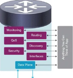
Figure 1.4: How software interacts with networks with onePK

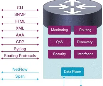
The idea of SDN attracted attention because of its applications in area of network monitor-ing and management. Currently networks are monitored/managed usmonitor-ing various protocols such as SNMP, Syslogs, NetFlow etc. We have our interest in the monitoring/management applica-tions as our goal, to maintain connectivity of a service, is essentially a network management application.

Figure 1.3 and Figure 1.4 shows the difference in how the monitoring/management approach is changed with introduction of SDN technologies, specifically onePK. We can see that non SDN approach has familiar toolkits, multiple knobs, controlled access and many special purpose tools but lacks a programmatic approach and has gaps and inconsistencies. With the use of SDN we can use modern programming languages to develop applications that seamlessly run across multiple platforms. We also have data plane interaction APIs which allow us to modify data plane packets thus extending our control [28].

1.5.2 Cisco ONE Platform Kit (onePK) API

Cisco introduced its SDN package in its Open Networking Environment (ONE) in 2011. The major difference between the open standards and Cisco is the open standard, OpenFlow, open up data path APIs whereas Cisco opened APIs to program all seven layers in its onePK.

Chapter 2

Algorithm Design

2.1

Problem Definition

To define the problem that we have solved in this report, we are giving working definitions of few terms. We will discussed these terms followed by the formal definition of the problem.

Virtual Service:

A virtual service is any application running on a virtual machine providing a service to its user. The virtual machine will be connected to the network through a VM host. For instance, Microsoft exchange server running on a VM inside a private NCSU cloud is a virtual service offered by NCSU’s private cloud.

Network Elements:

A network element is the network hardware which is used to provide access to the services offered by the network. Access, aggregation and core switches form good examples of network elements relevant to the discussion.

Given these definitions the problem definition is as follows:

Given migration of a virtual service from an initial placement to a final placement in a

hierarchical network designed as a Fat tree topology, can we find all the network elements that

NEED a state change [31] to support the migration?

Figure 2.1: Path from core switch to access switch connected to initial placement

Figure 2.3: DC-Tree of height four

reachability. The controller reprograms the network (green and orange elements) to support the migration i.e. maintains the service’s reachability after the change.

As a simple example, we can add the flow entries to the green elements and delete flow entries from the orange elements. This can be extended to program the network with other state information associated with the virtual application such as firewall rules, Access Control Lists (ACL), Virtual Local Area Network (VLAN) configuration etc.

Along with finding the elements that NEED a state change to support the migration, we are asking the following questions:

• Can we solve the problem without stringent restrictions on design of network fabric?

• Can we solve the problem without restrictions on IP address allocation?

• Can we solve the problem without need of new native hardware/software features?

While working on a solution, we mapped our problem to a new problem, that we call a

Common Root Problem. Once thecommon root problem is defined, we have discussed how solving it helps us solve our original problem of finding affected elements to support migration of a virtual service.

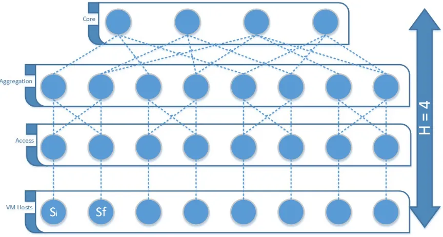
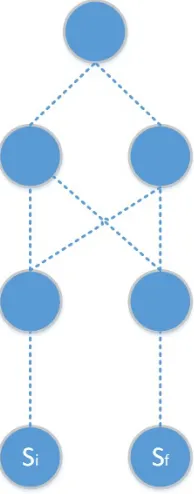
The common root problem is defined for a tree [9] (we call this tree a DC-Tree, see Fig-ure 2.3). DC-Tree is a tree with following properties:

1. Has maximum height of four

2. Can have multiple roots as long as it is a connected graph [9]

3. Has at least two leaves

DC-Tree tree is analogues to network topology of a hierarchical and modular virtual data centre where the root is a core element and leaves are the VM Hosts. The middle levels are the aggregation and access elements.

Being a connected graph [9] DC-Tree will always have a path between any of its leaves. If we trace a path from the source leaf to destination leaf we will start climbing up the hierarchy until we reach a point from which we can climb down to reach the destination leaf.

Considering the DC-Tree and this sub tree which takes us from the source to the destination

common root problem is defined as follows:

While travelling from a source leaf to a destination leaf in a DC-Tree can we find a

common root and elements of a feasible sub tree?

Solution of the common root problem solves the problem under consideration as follows:

• Source leaf can be our source VM host and the destination leaf can be our destination VM host

• The feasible sub tree is the path the migrating virtual application will take

• Elements of the sub tree that fall on the source side of the sub tree are the elements that need the delete operation of the virtual application state

• Elements of the sub tree that fall on the destination side of the sub tree are the elements that need the add operation of the virtual application state

for the state in consideration special care should be taking in choosing the sequence of add and delete operation to avoid invalid application state

Figure 2.4 shows an example of the source side sub tree, destination side sub tree and the common root.

Figure 2.4: DC-Tree with affected elements

2.2

Algorithm Definition

This section defines the algorithm as a pseudocode along with discussion on how the algorithm is validated followed by the validation.

2.2.1 Pseudocodes

called in the Algorithm 1. After each pseudocode we have presented discussion on the algorithm explaining its working, few comments along with its asymptotic analysis.

We claim Algorithm 1 is generic enough to support any topology as long as a topology has a modular hierarchical architecture, such as fat tree, Clos etc. i.e. if a topology can be reduced to a DC-Tree, Algorithm 1 should stand true to find the affected elements that NEED a state change to support the migration. Other algorithms give the idea of what is the expected output for given inputs by these algorithms and are written specific to the fat tree topology (shown in Figure 1.2a). They can be changed to make the implementation efficient based on the information of the environment.

Parent:

Parent of an element (saye) in a DC-Tree (see 3 on page 16) is an element which is higher in the hierarchy toe and will forward a packet destined fore to an element lower in the hierarchy so that it reachese

Child:

Child of an element (say e) in a DC-Tree (see 3 on page 16) is an element lower in hierarchy toe and usese as an immediate element to reach the root

Abstract Node:

An abstract node is a combination of two or more network elements of same level in hierarchy all of which are connected to a common element lower in the hierarchy. We have discussed abstract node, its uses in sections 2.2.3 and 2.3.

Algorithm 1 Find add, delete and modify lists of affected network elements

Input: Trigger of service migration provides source Si and destination Sf of the migrating service

Output: Add, delete and modify lists of network elements that NEED a state change to support the migration

Algorithm 1 starts with finding the parents of the source. This step gives information on which elements are utilized when a packet is sent to the source Si. This information helps us in finding all possible paths to/from Si. This is followed by node abstraction the reasons for which have been discussed. We have also discussed few applications of abstraction in section 2.3. The same process is repeated on Sf as we also need the information on possible paths to Sf. Once we have the information on the (abstracted) parents of both Si and Sf we can easily find a common root. Abstraction of nodes helps avoid a sub-tree splitting in two branches and eventually merging at some other point thus avoiding issues with the process to find common root. With the help of information on the parents and the common root we can proceed to find the expected output of add, delete and modify lists as per algorithms 5, 6 and 7.

Running time of Algorithm 1 depends on the running time of each of its step. We have discussed running time of each step is discussed after the proposed algorithm for that step. We have revisited running time analysis of Algorithm 1 after end of the last step - Algorithm 7. This running time analysis is done based onn→no. of ports on an elementand m→no. of modules of a f at tree. We have defined a module of a fat tree as shown in Figure 2.5

Figure 2.5: Fat tree module used for asymptotic analysis

By practical case analysis we mean analysis using values that are practical to today’s data centers. We feel such an analysis is essential as parameters used for analysis n and m, will take maximum values of few hundreds for n and less than 100 for m. These values are not computational intensive for today’s hardware even if running time is factorial, which is orders of magnitude greater than the actual running time of our algorithm.

We think that the communication delay will be significantly greater than the computational time in some of the cases and hence the practical cases analysis compares computational time of the algorithm with communication time.This analysis will help designers decide how the network application is deployed in the network so that they achieve best support

for virtualization.

Algorithm 2 Find parents in hierarchy of network elements→ FindParentsInHierarchy()

Input: Information of VM host (Si orSf)

Output: Parents of the VM host in the network hierarchy

1: AccessElemets=F indN eighborsOneLevelHighInHierarchy(S)∗

2: AggregationElements=F indN eighborsOneLevelHighInHierarchy(AccessElemets) 3: CoreElements=F indN eighborsOneLevelHighInHierarchy(AggregationElements)

Algorithm 2 gives us the information on all the parents as defined in the start of this sub-section. We start with finding the access elements as the service host will be directly connected to it. Once access is found aggregation can be found using Access (please note that access is used as a point in hierarchy while searching for parents of service host) and same can be done for core.

As discussed earlier in this section we have presented the worst case and practical case runtime analysis of Algorithm 2 —

Worst case analysis: Assuming the access switch has n ports and there are m modules in the fat tree. Withm modules, in the worst case aggregation switches will havem+ 2 (m

connections to core switches and 2 to access switches) active ports. Hence the running time of the algorithm will be O(n+m). As in normal cases n >> m we can say that Algorithm 2 will run inO(n).

Practical case analysis: If we consider one module at a time, an element will be connected to one access switch, access will be connected to two aggregation switches and each

ag-∗

gregation will be connected to at most m core switches. In a practical case, the uplink connections will be less costly than θ(n) as typically highest speed links are used for up-links. For instance, a switch will 1Gports will typically have two to four 10G links to be used as uplinks. With the use of such information the application can be made to find parents with m + 2 + 1 searches =⇒ running time of θ(1). As discussed earlier this will be insignificant considering the compute power typically available to programmers. Assuming a processor of 3GHz capacity, running though 100 numbers will not take more than few hundred nano seconds. Let us assume the computation takes 1µs.

A typical connection link in data center will have 1Gbps capacity and a onePK call to find Cisco Discovery Protocol (CDP) neighbour is 1622 bytes. This data size increases by about 153 bytes per new entry in the CDP table. With these numbers we can say that a call to find one neighbour will take about 12.9µsplus the queuing delays. Lets approximate this value to 10mswhich is a typical maximum allowed delay for real time applications in data centers [3]. We can see that, the computation is three orders of magnitude smaller than the connection time and hence we can conclude thatthe running time of Algorithm 2 will be affected by the connection time and not the computation time.

Algorithm 3 finds if node abstraction is required and if required it creates an abstract node, maintains the mapping of abstract node to its members and returns a list of elements which has all connected peers abstracted. As mentioned earlier algorithm can be changed as per implementation and depending on the environment factors. The main purpose of discussing Algorithm 3 is to give users an idea as to what is the expected behaviour of the algorithm.

We have list of all parents of an element as the input to the algorithm. Algorithm starts by sorting this list based on the hierarchy as the key and weight of value as Access<Aggregation

< Core. Depending on the input lists we can choose the most efficient algorithm for sorting. Once sorted we start by comparing the first element with the second, if they are equal (i.e. if they are connected peers) we add only the first element to a list which maintains mapping of abstract node to its members. This operation is indicated in Step 17 of Algorithm 3.

Considering the fat tree as shown in Figure 1.2a we will have at the most one abstract node per level and hence Algorithm 3 does not handled the case of having separate abstract nodes per level.

If the elements are unequal we have two possibilities: we have a non-abstract element or we have the last member element of the abstract node in consideration. We have used the

Algorithm 3 Abstract nodes when required→ IfRequiredAbstractNodes()

Input: List of peers in hierarchy as key-value pair (key being element identifier and value being one of access, aggregation or core)

Output: Modified list with peers grouped†

1: Initialize array of listsA[hierarchy][networkelements] .Hierarchy takes values access, aggregation or core

2: SORT(SiP arentsU ngroupped) . Sort based on the level in hierarchy of the element from access to core. Assume sorted list is SortedList.Si can be replaced bySf

3: counter←0 .counter keeps track of the duplicates free list, DFList 4: P artOf AbstractN ode=F ALSE .Flag to indicate an element is member of an abstract

node

5: if SiP arentsU ngroupped.length >1 then

6: for i:= 0→(SiP arentsU ngroupped.length−1)do

7: if SortedList[i]neq SortedList[i+ 1] then . Two abstract nodes are equal when their member elements have one-to-one match

8: if P artOf AbstractN odethen .If element is member of abstract node 9: A[hierarchy][hierarchy counter] =SortedList[i] . hierarchy counter+ + is separate counter to keep track of no. of access, aggregation and core elements. We can use three counters or single counter which resets when each level is completely explored

10: P artOf AbstractN ode=F ALSE .Resetting the flag as next element is not member of this abstract node

11: DF List[counter] =A[hierarchy] . Add abstract node to the duplicate free list

12: else

13: DF List[counter] =SortedList[i] . Add node to the duplicate free list

14: end if

15: counter+ +

16: else

17: A[hierarchy][hierarchy counter] =SortedList[i]

18: hierarchy counter+ +

19: P artOf AbstractN ode=T RU E

20: end if 21: end for 22: end if

23: DF List[counter] =SortedList[SiP arentsU ngroupped.length−1] . Always inserting last element into new array

In the first case i.e. if we have non-abstract element we avoid the costly insert operation to the list which maintains the mapping of abstract node to its members and directly add element to the list of duplicate free elements. Whereas in the second case i.e. if the element is the last member of an abstract node we add it to both the lists - list maintaining mapping of members to abstract node and duplicate free list.

Running time analysis for Algorithm 3 is presented below —

Worst case analysis: To calculate running time of the algorithm we can start with theSORT

operation. For worst case analysis of the algorithm lets assume there is no special knowl-edge about the data and we are sorting with running time of nlgn. We are sorting

SiP arentsU ngrouppedand maximum possible parents for any device would be 1 + 2 +m (maximum 1 access + maximum 2 aggregation per access + maximumm core elements) wheremis the number of modules. This implies theF OR in Step 6 will runm+ 2 times. In the worst case, we will have 1 compare and 1 insert operations for access elements, 3 compares and 1 + 2 inserts (one for insert in sorted list and two for inserts in members of a abstract node list) for aggregation elements and similarly m+ 1 comparisons and

m−1 + 2 inserts for core elements which adds up to 2m+ 10 operations and we have one final insert in Step 23. Adding it all up we have a running time ofO(m2).

Practical case analysis: In Algorithm 3 we are working on lists that are in memory i.e. there is no communication with network elements so we will not have any unlike Algorithm 2 we have a running time that is completely dependant on the computational time. But as discussed earlier, even tough the algorithm runs in second power of m for all practical purposes, the computational time will be insignificant. Implementation of this algorithm should make use of the knowledge of environment and possible data to make the compu-tation as fast as possible and Algorithm 3 should not affect the placement of the network application in the topology.

†

Algorithm 4 Find common root of two lists→ FindCommonRoot()

Input: List of elements of grouped parents of Si and Sf Output: Common root of lists‡

1: if AccessElement.SiP arents=AccessElement.SfP arents then 2: returnAccessElement.SiP arents

3: else if AggregationElement.SiP arents=AggregationElement.SfP arentsthen 4: returnAggregationElement.SiP arents

5: else

6: returnCoreElement.SiP arents 7: end if

The purpose of Algorithm 4 is to find the common root (as defined in section 2.1) amongst list of parents ofSi andSf. We start with list parents of Si andSf which has connected peers combined in abstract nodes. First step is comparison of access level elements. If common root is found at access level we need not go to higher levels as this will be the most efficient common root. We climb up to aggregation in step 3 and if aggregation is not the common root we can return core without an additional comparison.

If the first available common root is not the desired criteria this algorithm should be replaced accordingly.

Running time of Algorithm 4 is θ(1). This is already a very fast algorithm and in any practical case it should not affect the placement of network application in the data center.

Algorithm 5 Find list of elements that need add operation→ FindAddList()

Input: Information on the common root and list of elements in hierarchy of destination sub-strate

Output: Elements which need add operation

1: returngetChildrenOf Root(CommonRoot, SfP arents)

The purpose of Algorithm 5 is to find the list of elements that need ADD operation i.e. we need to add state to these elements to support the migration. The idea is basically all the elements that are children of common root in theSf parents sub tree. This is true as otherwise we should have found a different common root. So Algorithm 5 simply return children of common

‡

root in theSf parents sub tree.

Running time of Algorithm 5 is same as Algorithm 2 hence Algorithm 5 runs inO(n). The same argument as Algorithm 2 applies to Algorithm 5 in affecting the computational time and the placement of network application in the data center.

Algorithm 6 Find list of elements that need delete operation →FindDelList()

Input: Information on the common root and list of elements in hierarchy of source substrate Output: Elements which need delete operation

1: returngetChildrenOf Root(CommonRoot, SiP arents)

The purpose of Algorithm 6 is to find the list of elements that need DELETE operation i.e. we need to remove state from these elements to support the migration. It works similar to Algorithm 5. Here we return all the elements that are children of common root in theSi parents sub tree.

Running time of Algorithm 6 is same as Algorithm 2 hence Algorithm 6 runs inO(n). The same argument as Algorithm 2 applies to Algorithm 6 in affecting the computational time and the placement of network application in the data center.

Algorithm 7 Find list of elements that need modify operation→ FindModifyList()

Input: Information of elements that need both add and modify operations Output: Elements which need modify operation

1: returnCommonRoot .If anything other than common root should be part of this list, we have an error calculating common root

Algorithm 7 identifies the elements which were essential for communication with service before the migration and are also required after the migration. These elements are simply the elements which are part of both the ADD and DELETE lists and hence to find elements that need modification instead of ADD or DELETE Algorithm 7 iterates through both the lists to find common elements.

This algorithm is useful only if MODIFY operation is supported for the state that is being modified. If such operation is not supported we should simply DELETE followed by ADD or vice versa depending on the situation.

data center.

Asymptotic analysis of Algorithm 1 —

Worst case analysis: Considering the running time of Steps 1 through 8 of Algorithm 1 we can conclude the running time of Algorithm 1 to be O(n+m2).

If we look for the interpretation of the O(n+m2) value we can see that as the number of affected elements by the migration increases n will increase (as n will be total no. of port checked during one iteration of the algorithm) and m will stay constant. So we can conclude that as the number of affected elements increases the algorithms computational running time will increase. Its computation time will be significantly affected by the number of modules but this effect will be more or less constant and we can offset it with using smart deployment and design of the network application.

Practical case analysis: In a practical case, n >> m but m2 will be significant enough to affectnand hence the computational running time of Algorithm 1 will beO(n+m2)..

The computation time for Steps 1 through 8 of Algorithm 1 will still be very low, few hun-dredµsand because of Steps 1, 3, 6 and 7 i.e. Algorithm 2, Algorithm 5 and Algorithm 6 we will have significant communication wait times. For best performance the network and application designers should customize the application by applying techniques such as running the algorithm in a distributed fashion, periodic learning of the topology, making use of static data, making use of element properties that will not change etc. so that the no. of connections required to find possible parents of an element are reduced.

From point of view of memory only Algorithm 3 performs memory sensitive operations. We have array SORT, FIND, INSERT and DELETE operations. We have also suggested a multidi-mensional array to store hash map of abstract element with its member elements. In the worst case, Algorithm 3 can consume O(n2) memory where nis the number of parents ofSi orSf.

Software designers need to implement these structures based on their environment to keep memory consumption of the algorithm to minimum.

2.2.2 Validation Procedure

To validate the working of the algorithm we have taken a two fold approach:

1. Mathematical proofs

2. Experimental data

the claim of finding all affected network elements that NEED a state change to support the migration of the virtual application.

Mathematical proofs are presented in Section 2.2.3 as these present primary proof of the algorithm. The experiments are presented in Chapter 3.

2.2.3 Validation

As discussed earlier, in this report we are focusing on the fat tree architecture and hence all the validation arguments have been made from the point of view of fat tree. However, we have a claim that this algorithm is generic enough to be applied to other modular hierarchical architectures such as Clos which can be reduced to a DC-Tree without modifications. A NCSU student, Aditya Vaja, has validated this algorithm for Clos in an independent project [29]

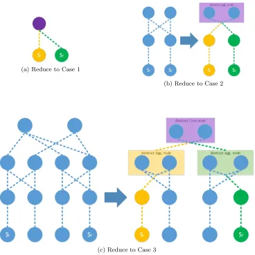
The goal of the algorithm Algorithm 1 (see page 18) isto find all the network elements that NEED a state change to support a virtual application migration. To validate that Algorithm 1 provides this information (provided in form of three lists: Add, Delete and Modify suggesting the operation to be performed on their member network elements) we have organized this section as follows: we start with definition of an abstract node which is essential for the algorithm to support equal cost multi paths (ECMPs) in the network. This definition is followed by reduction of all possible cases of paths fromSitoSf to three generic cases. Once we complete the reduction we have validated the algorithm by running through it step by step for each of the three generic cases with reasoning of why a particular output is expected (and given by the algorithm) for a given input. This completes the theoretical validation part which is followed by experimental support in chapter 3.

When a server or end host is connected in a fabric based of this tree, the path between the two for any given packet can be reduced to one of the three typologies shown in Figure 2.6. We have introduced a concept ofabstract node to aid this reduction. As defined earlier, anabstract node is a combination of two or more network elements of same level in hierarchy all of which are connected to a common element lower in the hierarchy.We will abstract network elements when an element lower or higher in the hierarchy can reach the destination through any of the

members of the abstract node and exactly which element is chosen doesn’t affect the algorithm. This does add a level of implementation complexity where we need to figure out the changes in members of abstract node especially when peers of the hierarchy are connected. The guarantee in an abstract node is the members will be affected. Abstract nodes also give us an opportunity to run specialized algorithm to choose an member element to satisfy requirements like traffic engineering.

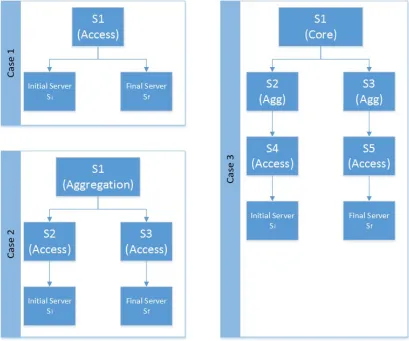
Figure 2.6: Three possible reductions of Fat tree

deletion, green indicates requirement of addition and purple indicates requirement of modifi-cation. An important point to note here is these path are not the actual connections but path that a TCP (or any other protocol under consideration) can take. It is possible that there is physical connectivity but the port is blocked by say Spanning Tree Protocol (SPT) then we are not taking this path in to account.

If Si and Sf are connected to the same access switch we have a trivial reduction to case 1 of Figure 2.6. This reduction is as shown in Figure 2.7a.

If the path from Si to Sf climbs up to the aggregation level and then starts climbs down the reduction is as per Figure 2.7b and hence we can place it in case two of Figure 2.6.

If the path from Si toSf climbs up to the core level and then climbs down the reduction is as per Figure 2.7c and hence we can place it in case three of Figure 2.6.

(a) Reduce to Case 1

(b) Reduce to Case 2

(c) Reduce to Case 3

Figure 2.7: Proof of reduction of all possible placements ofSi and Sf to three cases

exclusive from each other. This can be proved as follows: When a path exists from Si to Sf at access level in a connected graph [9] we will find a path from Si to Sf at aggregation and core levels but, as per Algorithm 4 discussed on page 24, we will have common root at access level instead of aggregation or core and hence these cases are mutually exclusive. Due to this behaviour it is important to consider path weights based on a criteria of choice (no. of hops, connection speed, congestion on the path etc.) when tracing paths. This also gives us a strong motivation to run algorithm on per migration basis.

algo-rithms function for all of these cases. We will run step by step through the algorithm and show that for a given input we are getting expected output with reasoning on why the expected out-put satisfies the claim of findingall the network elements that NEED a state change to support the migration. All the algorithms receive identifying information on the VM as inputs. This is represented by Si and Sf for source and destination respectively. This information can be any parameter which will allow us to trace a path from the source to destination which can be used by VM migration. An example can be IP address of the VM hosts, IP address of the VM etc.

Case 1 - Source and destination VM host is connected to the same access switch (see Fig-ure 2.6):

Input:

Si andSf can be any two distinct VM hosts connected to the same access switch. For the proof we are assumingSi and Sf both are connected to S1.

Output:

{AddList=φ},{DelList=φ} and {M odif yList=S1}

Discussion:

{AddList = φ} as the concerned access switch already has the state information so nothing new will be added, {DelList = φ} as the concerned access switch needs the state information so we cannot delete it and {M odif yList = S1} as the destination is connected to the same switch (access in this case) and we need to MODIFY the mapping of state information to point from the old VM host to the new VM host.

Another way of interpreting AddList, DelList and the ModifyList is these are the elements that NEED a state change to support the migration. With the state information in S1 modified to point to the new location of the virtual service, network will bring the traffic according to the existing rules till S1 and S1 will take action according to the modified information thus supporting the migration.

Proof:

Algorithm 1 Step 1: F indP arentsInHierarchy(Si) Algorithm 2 Step 1: AccessElements=S1 Algorithm 2 Step 2: AggregationElements=φ

Algorithm 2 Step 3: CoreElements=φ

Return value:SiP arentsU ngrouped=S1

Algorithm 1 Step 2: If RequiredAbstractN odes(SiP arentsU ngrouped→S1) Algorithm 3 Step 1: A[access][ ]→N U LL, A[aggregation][ ]→N U LL,

Algorithm 3 Step 2: SortedList=SORT(S1) Algorithm 3 Step 3: counter→0

Algorithm 3 Step 4: P artOf AbstractN ode→F ALSE

Algorithm 3 Step 5: IFSiP arentsU ngroupped.length >1→FALSE go toEND IF

Algorithm 3 Step 23:DF List[0] =S1

Return value:SiP arents={S1}, A Algorithm 1 Step 3: same as Step 1

Return value:SfP arentsU ngrouped=S1 Algorithm 1 Step 4: same as Step 2

Return value:SfP arents={S1}, A

Algorithm 1 Step 5: FindCommonRoot(SiP arents,SfP arents) Algorithm 4 Step 1: IFAccessElements.SiP arents=

AccessElements.SfP arents→ TRUE

Algorithm 4 Step 2: return AccessElements.SiP arents Return value:CommonRoot=S1

Algorithm 1 Step 6: FindAddList(CommonRoot,SfP arents)

Algorithm 5 Step 1: getChildrenOfRoot(CommonRoot,SfP arents)

Return value:AddList=φ

Algorithm 1 Step 7: FindDelList(CommonRoot,SiP arents) 6 Step 1: getChildrenOfRoot(CommonRoot,SiP arents)

Return value:DelList=φ

Algorithm 1 Step 8: FindModifyList(CommonRoot) Return value:M odif yList=S1

End of case 1:

We have found the result as expected -{AddList=φ}, {DelList=φ} and

{M odif yList=S1}

Case 2 - Source and destination VM host is connected to the same access switch (see Fig-ure 2.6):

Input:

and necessarily to distinct access switches. For sake of the proof we are assuming Si to be connected to S2 andSf to S3. S2 and S3 are connected by S1 at aggregation level. Output:

{AddList=S3},{DelList=S2} and {M odif yList=S1}

Discussion:

{AddList=S3}asSf is connected to S3 and we need S3 to have state information of the virtual service to support the migration,{DelList=S2}asSi is connected to S2 and we no longer need S2 to have state information for the virtual service, in fact S2 having state information can cause issues due to stale data and {M odif yList = S1} as the source and destination switches, S2 and S3 respectively, are connected to S1 (aggregation in this case) and we need to MODIFY the mapping of state information to point from S2 to S3 to support the migration.

As discussed earlier, another way of interpreting AddList, DelList and the ModifyList is these are the elements that NEED a state change to support the migration. With the state information added to S3, removed from S2 and modified in S1 modified to point to the new location of the virtual service. The traffic that comes to S2 so as to reach the service due to stale information will not find the service connected to S2 (as we have removed the state from S2) and will start looking for the location based on existing algorithms. As soon as it reaches S1 we get a direction and required state to reach the service via S3. Similarly, the traffic that was trying to reach the service via S1 or S3 (eg. come to S1/S3 then go towards S2 to reach the service) will now be able to access the service without any issues thus supporting the migration.

Proof:

Algorithm 1 Step 1: F indU ngrouppedP arents(Si) Algorithm 2 Step 1: AccessElements=S2 Algorithm 2 Step 2: AggregationElements=S1 Algorithm 2 Step 3: CoreElements=φ

Return value:SiP arentsU ngrouped=S2, S1

Algorithm 1 Step 2: If RequiredAbstractN odes(SiP arentsU ngrouped) Algorithm 3 Step 1: A[access][ ]→N U LL, A[aggregation][ ]→N U LL,

A[core][ ]→N U LL

Algorithm 3 Step 2: SortedList=SORT(S2, S1) Algorithm 3 Step 3: counter→0

Algorithm 3 Step 5: IFSiP arentsU ngroupped.length >1→ TRUE

Algorithm 3 Step 6: FOR i = 0 → (SiP arentsU ngrouped.length−1) → TRUE

Algorithm 3 Step 7:IF SortedList[0] neq SortedList[1]→TRUE Algorithm 3 Step 8:IF P artOf AbstractN ode→ FALSEgo to Step 13 Algorithm 3 Step 13:DF List[0] =S2

Algorithm 3 Step 15:counter = 1→go to Step 6

Algorithm 3 Step 6: FOR i = 0 → (SiP arentsU ngrouped.length−1) → FALSE go to Step 23

Algorithm 3 Step 23:DF List[1] =S1 Return value:SiP arents={S2, S1}, A Algorithm 1 Step 3: same as Step 1

Return value:SfP arentsU ngrouped=S3, S1 Algorithm 1 Step 4: same as Step 2

Return value:SfP arents={S3, S1}, A

Algorithm 1 Step 5: FindCommonRoot(SiP arents,SfP arents) Algorithm 4 Step 1: IFAccessElements.SiP arents=

AccessElements.SfP arents→ FALSEgo to Step 3 Algorithm 4 Step 3: IFAggregationElements.SiP arents=

AggregationElements.SfP arents→ TRUE

Algorithm 4 Step 4: return AggregationElements.SiP arents Return value:CommonRoot=S1

Algorithm 1 Step 6: FindAddList(CommonRoot,SfP arents)

Algorithm 5 Step 1: getChildrenOfRoot(CommonRoot,SfP arents) Return value:AddList=S3

Algorithm 1 Step 7: FindDelList(CommonRoot,SiP arents) 6 Step 1: getChildrenOfRoot(CommonRoot,SiP arents) Return value:DelList=S2

Algorithm 1 Step 8: FindModifyList(CommonRoot) Return value:M odif yList=S1

End of case 2:

We have found the result as expected -{AddList=S3}, {DelList=S2} and

Case 3 - Source and destination VM host is connected to the same access switch (see Fig-ure 2.6):

Input:

Si and Sf can be any two distinct VM hosts connected to the same core switch and nec-essarily to different access and aggregation switch. For sake of the proof we are assuming

Si to be connected to S4 andSf to S5 in Figure 2.6. S4 is connected to S2 at aggregation level and S5 is connected to S3 at aggregation level. S2 and S3 are connected to each other via core switch S1.

Output:

{AddList=S3, S5},{DelList=S2, S4} and {M odif yList=S1}

Discussion:

{AddList = S3, S5} as Sf is directly connected to S5 and we need S3 and S5 to have state information of the virtual service to support the migration, {DelList=S2, S4}as

Si is directly connected to S5 and we no longer need S2 and S5 to have state information for the service, in fact S2 and S4 having state information can cause issues due to stale data and{M odif yList=S1}as the source and destination aggregation switches, S2 and S3 respectively, are connected to S1 (core switch in this case) and we need to MODIFY the mapping of state information to point from S2 to S3 to support the migration of the virtual service.

As discussed earlier, another way of interpreting AddList, DelList and the ModifyList is these are the elements that NEED a state change to support the migration. Similar to the discussion for Case 1 and Case 2 we can show that with addition of information to S3 and S5, deleting it from S2 and S4 and modifying it in S1 we can support the migration.

Proof:

Algorithm 1 Step 1: F indU ngrouppedP arents(Si) Algorithm 2 Step 1: AccessElements=S4 Algorithm 2 Step 2: AggregationElements=S2 Algorithm 2 Step 3: CoreElements=S1

Return value:SiP arentsU ngrouped=S4, S2, S1

Algorithm 1 Step 2: If RequiredAbstractN odes(SiP arentsU ngrouped) Algorithm 3 Step 1: A[access][ ]→N U LL, A[aggregation][ ]→N U LL,

A[core][ ]→N U LL

Algorithm 3 Step 4: P artOf AbstractN ode→F ALSE

Algorithm 3 Step 5: IFSiP arentsU ngroupped.length >1→ TRUE

Algorithm 3 Step 6: FOR i = 0 → (SiP arentsU ngrouped.length−1) → TRUE

Algorithm 3 Step 7:IF SortedList[0] neq SortedList[1]→TRUE Algorithm 3 Step 8:IF P artOf AbstractN ode→ FALSEgo to Step 13 Algorithm 3 Step 13:DF List[0] =S4

Algorithm 3 Step 15:counter = 1→go to Step 6

Algorithm 3 Step 6: FOR i = 0 → (SiP arentsU ngrouped.length−1) → TRUE

Algorithm 3 Step 7:IF SortedList[1] neq SortedList[2]→FALSE Algorithm 3 Step 8:IF P artOf AbstractN ode→ FALSEgo to Step 13 Algorithm 3 Step 13:DF List[1] =S2

Algorithm 3 Step 15:counter = 2→go to Step 6

Algorithm 3 Step 6: FOR i = 0 → (SiP arentsU ngrouped.length−1) → FALSE go to Step 23

Algorithm 3 Step 23:DF List[2] =S1

Return value:SiP arents={S4, S2, S1}, A Algorithm 1 Step 3: same as Step 1

Return value:SfP arentsU ngrouped=S5, S3, S1 Algorithm 1 Step 4: same as Step 2

Return value:SfP arents={S5, S3, S1}, A

Algorithm 1 Step 5: FindCommonRoot(SiP arents,SfP arents) Algorithm 4 Step 1: IFAccessElements.SiP arents=

AccessElements.SfP arents→ FALSEgo to Step 3 Algorithm 4 Step 3: IFAggregationElements.SiP arents=

AggregationElements.SfP arents→ FALSE go to Step 6 Algorithm 4 Step 6: return CoreElements.SiP arents

Return value:CommonRoot=S1

Algorithm 1 Step 6: FindAddList(CommonRoot,SfP arents)

Algorithm 5 Step 1: getChildrenOfRoot(CommonRoot,SfP arents)

Return value:AddList=S3, S5

6 Step 1: getChildrenOfRoot(CommonRoot,SiP arents)

Return value:DelList=S2, S4

Algorithm 1 Step 8: FindModifyList(CommonRoot) Return value:M odif yList=S1

End of case 3:

We have found the result as expected - {AddList = S3, S5}, {DelList = S2, S4} and

{M odif yList=S1}

As a final note, on the theoretical validation section we would like to discuss why we think this algorithm successfully achieves our goals. These are the same questions that we asked while defining the problem in Section 2.1.

When we started thinking about the problem of finding all network elements that need a state change to support a virtual service migration there was an important consideration to keep in mind, the solution should be practical to implement without affecting the existing network environment. We did not want to propose a solution which restricts designers with requirements similar to those listed below —

• Specific design of network fabric. Till now we can say with confidence that we can support at least one forms of modular and hierarchical architectures: fat tree and it is well known that designers have lot of other motivating factors to choose such designs. Claim is we should be able to reduce any modular hierarchical network to a DC-tree but we have not yet validated the claim on other similar topologies and it is a work in progress

• Restrictions on IP addressing, in fact we don’t even need the network to be TCP/IP

• Need to add new native hardware features

• Restrictions on virtual service migration domain

The proposed Algorithm 1 imposes only two conditions:

• Topology should be reducible to DC-Tree

• For any practical importance we should be able to find parents and children of network elements along a service migration path

2.3

Discussion

The focus of this section is discussion on how some of the claims made in this chapter are possible. We have tried to prove and validate the claims as and when we made them. This section focuses on two claims proving which would have been too length and slightly out of context for the discussion.

Claim 1: Algorithm can be extended to other modular hierarchical topologies like Clos As the name suggests, modular and hierarchical topologies have small modules of hier-archical elements which are repeated. These topologies are highly scalable and easy to maintain hence they are very popular in data centre architectures.

To apply the algorithm to any modular hierarchical design we start by finding a suitable size module which can act as an independent entity. For instance, in the fat tree we have single core switch with block of two aggregation and two access switches as a possible module. We have leveraged this module in the proofs as well as the implementation. Once we drill down to such a module generic implementation of functions that form Algorithm 2, Algorithm 3 can be implemented. Once we have the information of the grouped parents, Algorithm 4, Algorithm 5 and Algorithm 6 can be computed and as Algorithm 7 takes inputs from Algorithm 5 and Algorithm 6 it can also be computed.

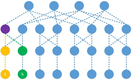
Let us discuss this claim using an example of Clos topology. Figure 2.8 shows a DC-tree which represents Clos as shown in Figure 1.2b of Chapter 1. We can see that we have tree of height four where the top level can be similar to the core followed by aggregation and access where the bottommost level being the VM hosts.

In this particular case we will consider each level as a module. Assuming we want to migrate from VM host 13 to VM host 15 we will be able to see the outputs of Algorithm 1 as follows:

Algorithm 1 Step 1: SiP arentsU ngroupped={9,5,6,7,8,1,2,3,4}

Algorithm 1 Step 2: SiP arents={9,{AbstractN odeW ithM embers{5,6,7,8}},

{AbstractN odeW ithM embers{1,2,3,4}}}

Algorithm 1 Step 3: SfP arentsU ngroupped={11,5,6,7,8,1,2,3,4}

Algorithm 1 Step 4: SfP arents={11,{AbstractN odeW ithM embers{5,6,7,8}},

{AbstractN odeW ithM embers{1,2,3,4}}}

Algorithm 1 Step 5: CommonRoot={AbstractN odeW ithM embers{5,6,7,8}}

Algorithm 1 Step 6: AddList= 11 Algorithm 1 Step 7: DelList= 9

Algorithm 1 Step 8: M odif yList={AbstractN odeW ithM embers{5,6,7,8}}

Claim 2: Abstract node can be used to apply specialized algorithms to perform functions such as load balancing, traffic engineering etc. on its member elements.

If we use Figure 2.9 as a reference figure, there are two points which facilitate Claim 2. If we focus our attention at the point between say node 3 to the abstract node, this is the point where we should run our special algorithms for ingress traffic to abstract node members node 1 and node 2. Similarly the egress traffic can be concentrated at another virtual point between aggregation and core levels to run egress algorithms.