Comparative Analysis of Dispersion Models for Waste Stabilization Pond

(1)

ISSN(Online): 2319-8753

ISSN (Print): 2347-6710

I

nternational

J

ournal of

I

nnovative

R

esearch in

S

cience,

E

ngineering and

T

echnology

(An ISO 3297: 2007 Certified Organization)

Vol. 4, Issue 12, December 2015

Comparative Analysis of Dispersion Models

for Waste Stabilization Pond

Uneke Louis Agwu, Akpan Paul Paulinus

Department of Civil Engineering, Rivers State Polytechnic, Bori-Nigeria, West Africa

ABSTRACT: Five dispersion models used in the determination of dispersion number (d) using experimental results obtained from a laboratory channel. Model calculations show that Liu’s model is closest to Levenspiel’s model which is used as standard for tracer concentration measurement in ponds. Lui’s model may then be used for design of new ponds. Agunwamba’s model follows after Liu’s in closeness to the measured, but is better than Levenspiels in that it is time saving and cost effective. However, unlike Liu’s model Agunwamba’s model cannot be used in design of new ponds.

KEYWORD: Waste stabilization pond, Dispersion coefficient, Model, Pollution, Treatment unit, Average velocity, Flow time

I INTRODUCTION

Much of the waste generated by man find their way into streams and rivers untreated. Raw sewage is often treated in waste stabilization pond (WSP) where such ponds are available. A poorly designed WSP results in heavy pollution. An important parameter for the design of wastewater treatment units and evaluation of the assimilatory capacity of stream is the dispersion coefficient D.

Many models have been developed for dispersion coefficient or its dimensionless equivalent called dispersion number,

defined as



0 d



. There is however no accepted method of determining dispersion coefficient as there is usually a

wide disparity between measured values of dispersion coefficient. Using [1] method and the predictive models. The paper is a comparative investigation of these models with intent of finding which of them relates closest to the measured value.

II REVIEW OF DISPERSION MODEL

Models for the determination of the dispersion coefficient may be classified into two group according to their specific input data requirement [2].

Those that require only pond geometry and flow conditions, [3]. This group does not require measurement on existing pond flow and consequently can be used in the design of new ponds. The group include the predictive model

Those that depend on the measurement of existing ponds (Levenspiel and Smith) and Aguamba consequently not used in the design of new ponds.

A. Levenspiel and Smith (1957) Model.

This model is based n the one-dimensional equation given as

x

c

U

x

c

D

t

c







₂2 (1)

(2)

ISSN(Online): 2319-8753

ISSN (Print): 2347-6710

I

nternational

J

ournal of

I

nnovative

R

esearch in

S

cience,

E

ngineering and

T

echnology

C= tracer concentration, D= tracer dispersion coefficient, U= average velocity, x= distance along river stretch from inlet

t=time of flow

The solution of the equation is given as







1



2 2 1 1

4 exp

4

1 d

ut

x

td

M

Cv









(2) Where,

M= mass of tracer injected, V=volume of wastewater, Q=flow rate,

d

₁= dispersion number=

uL

D



, L= pond length

and



= dimensionless time

V

Qt

.

The normalised variance as given by Levenspiel and Smith using the movement method is

2 2 2

)

(

)

(



_



_













m

CV

m

cv

(3)

The relationship between nomarlised varience and dispersion was obtained as [1]









_



(

8

1 )

1

8

1

1₂

2



d

(4)

Where



















1 



2





i i i

C

(5)

This is the conventional method of determining the coefficient of dispersion.

B. Liu (1977) Model [4]_{modified fisher’s formular into}

A

U

w

U

D

X 2





(6)

After experimentally finding the value of



, Liu’s assuming wide channel gave his formular as

 









1.25 25 . 0

2

168 .

0 Lwh

h

w

d







(7)

Polprasert and Bhahatarai argued that Lui’s assumption of wide channels was not applicable to pond and gave their model as

Lh

U

Uw

d

X 2 2





(8)

And solving arrived at

 





0.489 1.511

2

184 .

0 w

h

w

(3)

ISSN(Online): 2319-8753

ISSN (Print): 2347-6710

I

nternational

J

ournal of

I

nnovative

R

esearch in

S

cience,

E

ngineering and

T

echnology

UL

D

d



C

(10) Where x C

6.93hU

D



2 1 x

3 f

U

















e

R

24 f



Re= Reynold’s number= 2L



= Kinematic viscosity= 0.897x10-6 m2/s

C. Agunwamba (2011) Model

Agunwamba’s model is based on moment method at constant sampling time and variable distance [5]

. The equation is





_

























































2 1 2 2 2 2 1 2

2 exp

2

1

4 exp

D

t

u

Dt

t

u

D

t

u

Dt

Ut



2 2 2 1

4 exp

2 



_







































D

t

u

Dt

D

t

u

evfc

u

Dt

Ut



(11)

The variance is given as

2 2





















c

cx

c

cx



(12)

The value of D in this paper was obtained by computer programming III METHODOLOGY

Equipment and material used include a channel 14.0m long, 0.4m wide and 0.23m deep; a weighing balance; sodium chloride and a current meter. Salt weighing 400grams of salt was measured out and dissolved in 200 ml of water. The solution was introduced at the inlet of the channel with water flowing at a determined velocity. The samples were collected in two different ways.

First, samples were collected simultaneously at regular interval of 2.0m along the channel length. This represents the constant time variable distance method. The experiment was repeated at other determined velocities to obtain the constant time-variable distance data.

In the second method the salt solution was introduced at the channel inlet and collected at outlet at varying times representing the theoretical detention time of the channel. This is the constant distance, variable time method. The experiment was repeated nine times at the same velocity as in the first case.

(4)

ISSN(Online): 2319-8753

ISSN (Print): 2347-6710

I

nternational

J

ournal of

I

nnovative

R

esearch in

S

cience,

E

ngineering and

T

echnology

using the various models and plotted against distance. These were compared with the measured value calculated by Leverspiel and smith equation. The constant time variable distance plot was based on Agunwamba’s model.

IV RESULTS AND DISCUSSIONS

Table 1: Table of Dispersion Numbers for Various Models

Levenspiel and smith

Liu Polprasert and

Bhattarai

Taylor Agunwamba

1. 8.2709E-2 7.6571E-2 2.6025E-4 4.788E-5 6.8051E-2

2. 4.2576E-2 7.2785E-2 1.3831E-4 9.026E-5 1.4770E-1

3. 9.0176E-2 7.0765E-2 8.8210E-5 1.378E-4 1.748E-1

4. 5.8501E-2 7.4852E-2 7.2575E-5 1.717E-4 1.4301E-1

5. 1.2588E-1 7.1382E-2 1.8693E-4 8.925E-5 2.420E-1

6. 1.2025E-1 7.9545E-2 5.2101E-5 2.396E-4 2.5030E-1

7. 1.4953E-1 8.4186E-2 2.2998E-5 2.918E-4 3.0240E-1

8. 1.2793E-1 8.5712E-2 3.8811E-5 3.203E-4 3.0990E-1

9. 6.2686E-1 8.8562E-2 3.4627E-5 3.573E-4 3.0270E-1

Table 1 shows the results of dispersion coefficients for the five models considered. Liu’s model gave values closest to the measured, followed by Agunwamba’s. Polprasert and Bhattarai and Taylor’s models gave values much less than the measured and nearly zero. Generally, the table does not follow a regular trend and so does not lead to a conclusion between Liu and Agunwamba models. Undulations may be owing to incomplete mixing and low resistance of tracer material to adsoption7.

The concentration-time curves for Levenspiel and Liu (Plate 1-9) follow same pattern with characteristic long tails rising from zero after a long time, to a peak and then falling back to zero. The curves for Polprasert and Taylor run in straight lines at zero level for most of the experiments. This gives the impression of a plug flow which describes an ideal condition[6].

Tables and Plots Concentration Time Curves Existing for Dispersion Models for Experiments 1-9

Table I: Experiment 1A

Time (s)

Levenspiel(Cm) (mg/l)

Liu(Cp) (mg/l)

Polprasert(Cp) (mg/l)

Taylor(Cp) (mg/l)

0 0 0 0.00 0.00

6 0 0 0.00 0.00

12 0 0 0.00 0.00

18 0 0 0.00 0.00

24 0 5 0.00 0.00

30 0.14 0.42 0.00 0.00

36 1.95 1.9 0.00 0.00

42 3.18 2.45 0.27 0.02

48 1.33 1.43 0.00 0.00

54 0.23 0.49 0.00 0.00

(5)

ISSN(Online): 2319-8753

ISSN (Print): 2347-6710

I

nternational

J

ournal of

I

nnovative

R

esearch in

S

cience,

E

ngineering and

T

echnology

Plate 1: Experiment 1A

In the concentratiion-time curves for plate 1 in experiment 1A comparing existing dispersion models for waste-stabilization ponds, Liu agrees better with measured and both of the more realistic. Table 1 showed that Taylor, Proprasert, Liu and Levenspiel had maximum concentration of 0.02, 0.27, 5.00, and 3.18 mg/l respectively. The curve presented in plate one showed that Liu had the best curve that agrees is almost in a straight line.

Table 2: Experiment 2A

Time (s)

Liu(Cp) (mg/l)

Taylor(Cp) (mg/l)

0 0.00 0.00 0.00 0.00

5 0.00 0.00 0.00 0.00

10 0.00 0.00 0.00 0.00

15 0.00 0.00 0.00 0.00

20 0.00 5.00 0.00 0.00

25 0.14 0.42 0.00 0.00

30 1.95 1.90 0.00 0.00

35 3.18 2.45 0.27 0.02

40 1.33 1.43 0.00 0.00

45 0.23 0.49 0.00 0.00

50 0.20 0.12 0.00 0.00

(6)

ISSN(Online): 2319-8753

ISSN (Print): 2347-6710

I

nternational

J

ournal of

I

nnovative

R

esearch in

S

cience,

E

ngineering and

T

echnology

Liu agrees better with the measured, both more realistic in plate 2 while Table 2 gave approximately same result presented in Table 1

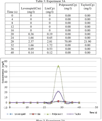
Table 3: Experiment 3A

Time (s)

Liu(Cp) (mg/l)

Taylor(Cp) (mg/l)

0 0 0 0.00 0.00

4 0 0 0.00 0.00

8 0 0 0.00 0.00

12 0 0 0.00 0.00

16 0 0 0.00 0.00

20 0.36 0.19 0.00 0.00

24 1.66 0.65 0.00 0.00

28 2.37 2.81 70.89 21.90

32 1.66 1.72 0.00 0.00

36 0.69 0.53 0.00 0.00

40 0.14 0.12 0.00 0.00

(7)

ISSN(Online): 2319-8753

ISSN (Print): 2347-6710

I

nternational

J

ournal of

I

nnovative

R

esearch in

S

cience,

E

ngineering and

T

echnology

TableIV: Experiment 4A

Time (s)

Liu(Cp) (mg/l)

Taylor(Cp) (mg/l)

0 0 0 0.0 0.0

4 0 0 0.00 0.00

8 0 0 0.00 0.00

12 0 0 0.00 0.00

16 0.01 0.04 0.00 0.00

20 1.09 1.26 0.00 0.00

24 3.33 2.95 28.82 52.48

28 1.4 1.47 0.00 0.00

32 0.17 0.28 0.00 0.00

36 0 0.03 0.00 0.00

40 0 0.02 0.00 0.00

In plate 4A Proprasert and Taylor agree better and are more realistic than the observed shape of both measured and Liu. Table 4 showed that Taylor, Proprasert, Liu and Levenspiel had maximum concentration of 52.48, 28.82, 2.95, and 3.33 mg/l respectively.

Table V: Experiment 5A

Time (s)

Liu(Cp) (mg/l)

Taylor(Cp) (mg/l)

0 0 0 0.00 0.00

4 0 0 0.00 0.00

8 0 0 0.00 0.00

12 0 0 0.00 0.00

16 0.31 0.26 0.00 0.00

20 4.83 1.87 0.00 0.00

24 2.19 2.29 0.00 0.00

(8)

ISSN(Online): 2319-8753

ISSN (Print): 2347-6710

I

nternational

J

ournal of

I

nnovative

R

esearch in

S

cience,

E

ngineering and

T

echnology

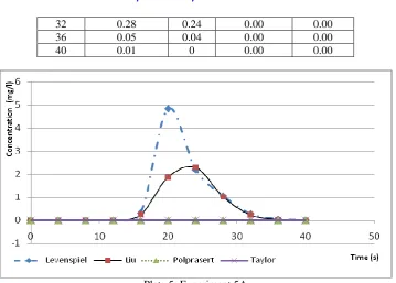
32 0.28 0.24 0.00 0.00

36 0.05 0.04 0.00 0.00

40 0.01 0 0.00 0.00

Plate 5A showed that Liu and measured are better related straight line of Polprasert and Taylor showed ideal situation and therefore unrealistic. Table 4 showed that Taylor, Proprasert, Liu and Levenspiel had maximum concentration of 0.00, 0.00, 2.29, and 4.83 mg/l respectively.

Table VI: Experiment 6A

Time (s)

Liu(Cp) (mg/l)

Taylor(Cp) (mg/l)

0 0 0 0.0 0.0

3 0 0 0.00 0.00

6 0 0 0.00 0.00

9 0 0 0.00 0.00

12 0.3 0.01 0.00 0.00

15 0.52 0.23 0.00 0.00

18 0 2.16 0.00 0.00

21 2.34 2.94 0.00 0.00

24 1.3 1.2 0.00 0.00

27 0.44 0.11 0.00 0.00

(9)

ISSN(Online): 2319-8753

ISSN (Print): 2347-6710

I

nternational

J

ournal of

I

nnovative

R

esearch in

S

cience,

E

ngineering and

T

echnology

In plate 6 the measured and Liu curves prove to be better and more realistic than Polprasert and Tailor. Table 4 showed that Taylor, Proprasert, Liu and Levenspiel had maximum concentration of 0.00, 0.00, 2.94, and 2.34 mg/l respectively.

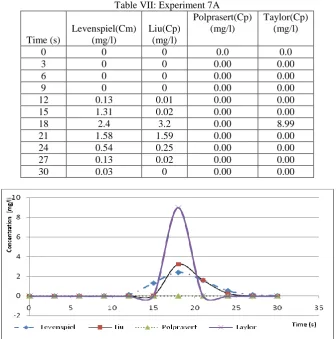
Table VII: Experiment 7A

Time (s)

Liu(Cp) (mg/l)

Taylor(Cp) (mg/l)

0 0 0 0.0 0.0

3 0 0 0.00 0.00

6 0 0 0.00 0.00

9 0 0 0.00 0.00

12 0.13 0.01 0.00 0.00

15 1.31 0.02 0.00 0.00

18 2.4 3.2 0.00 8.99

21 1.58 1.59 0.00 0.00

24 0.54 0.25 0.00 0.00

27 0.13 0.02 0.00 0.00

30 0.03 0 0.00 0.00

(10)

ISSN(Online): 2319-8753

ISSN (Print): 2347-6710

I

nternational

J

ournal of

I

nnovative

R

esearch in

S

cience,

E

ngineering and

T

echnology

In Plate 7A Taylor, measured and Liu showed good agreement while Proprasert does not. Table 4 showed that Taylor, Proprasert, Liu and Levenspiel had maximum concentration of 8.99, 0.00, 3.20, and 2.40 mg/l respectively.

Table VIII: Experiment 8A

Time (s)

Liu(Cp) (mg/l)

Taylor(Cp) (mg/l)

0 0 0 0.0 0.0

3 0 0 0.00 0.00

6 0 0 0.00 0.00

9 0 0 0.00 0.00

12 0.12 0.03 0.00 0.00

15 1.57 1.42 0.00 0.00

18 2.6 3.15 0.00 5.75

21 1.29 1.15 0.00 0.00

24 0.3 0.14 0.00 0.00

27 0.04 0.01 0.00 0.00

30 0 0 0.00 0.00

Tailor, measured and Liu also show good agreement while Proprasert does not in plate 8A. Taylor, Proprasert, Liu and Levenspiel had maximum concentration of 5.75, 0.00, 3.15, and 2.60 mg/l respectively in Table 8A.

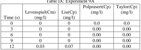
Table IX: Experiment 9A

Time (s)

Liu(Cp) (mg/l)

Taylor(Cp) (mg/l)

0 0 0 0.0 0.0

3 0 0 0.00 0.00

(11)

ISSN(Online): 2319-8753

ISSN (Print): 2347-6710

I

nternational

J

ournal of

I

nnovative

R

esearch in

S

cience,

E

ngineering and

T

echnology

15 2.03 2.09 0.00 0.00

18 3.17 2.79 0.00 0.00

21 0.43 0.65 0.00 0.00

24 0 0.05 0.00 0.00

27 0 0 0.00 0.00

30 0 0 0.00 0.00

Liu and measured are in good aggreement in plate 9 while Taylor, Proprasert, Liu and Levenspiel had maximum concentration of 0.00, 0.00, 2.79, and 3.17 mg/l respectively in Table 9A

Table X: Experiment. 1B

Distance (X)

Measured Concentration

Cm (mg/l)

Predicted Concentration

Cp (mg/l)

0 0.00 0.00

2 0.00 0.00

4 9.95 0.00

6 0.32 0.00

8 0.10 0.02

10 0.00 0.30

12 0.00 3.25

14 0.00 2.64

16 0.00 0.16

18 0.00 0.00

20 0.00 0.00

22 0.00 0.00

(12)

ISSN(Online): 2319-8753

ISSN (Print): 2347-6710

I

nternational

J

ournal of

I

nnovative

R

esearch in

S

cience,

E

ngineering and

T

echnology

Plate 10: Experiment 1B

Plate 10 showed good aggreement between Agunwamba and measured. Table 10 showed that the Agunwamba and measured had maximum concentration of 3.25 and 9.95 respectively.

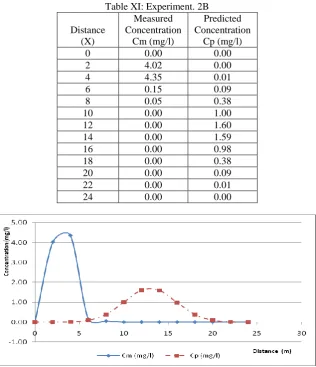
Table XI: Experiment. 2B

Distance (X)

Cm (mg/l)

Cp (mg/l)

0 0.00 0.00

2 4.02 0.00

4 4.35 0.01

6 0.15 0.09

8 0.05 0.38

10 0.00 1.00

12 0.00 1.60

14 0.00 1.59

16 0.00 0.98

18 0.00 0.38

20 0.00 0.09

22 0.00 0.01

(13)

ISSN(Online): 2319-8753

ISSN (Print): 2347-6710

I

nternational

J

ournal of

I

nnovative

R

esearch in

S

cience,

E

ngineering and

T

echnology

Plate 11 showed good agreement between Agunwamba and measured. Agunwamba and measured had maximum concentration of 1.60 and 4.35 respectively In Table 11.

Table X II: Experiment. 3B

Distance (X)

Cm (mg/l)

Cp (mg/l)

0 0.00 0.00

2 3.19 0.00

4 0.15 0.00

6 5.00 0.07

8 2.50 0.34

10 0.00 0.95

12 0.00 1.60

14 0.00 1.65

16 0.00 1.06

18 0.00 0.42

20 0.00 0.10

22 0.00 0.02

24 0.00 0.00

Plate 12 showed good agreement between Agunwamba and measured. In table 11 the maximum concentration for Agunwamba and measured are 1.65 and 5.00 respectively.

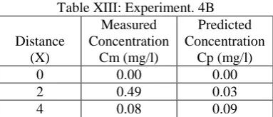
Table XIII: Experiment. 4B

Distance (X)

Cm (mg/l)

Cp (mg/l)

0 0.00 0.00

2 0.49 0.03

(14)

ISSN(Online): 2319-8753

ISSN (Print): 2347-6710

I

nternational

J

ournal of

I

nnovative

R

esearch in

S

cience,

E

ngineering and

T

echnology

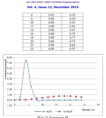
6 0.03 0.18

8 0.00 0.30

10 0.00 0.43

12 0.00 0.56

14 0.00 0.67

16 0.00 0.75

18 0.00 0.77

20 0.00 0.74

22 0.00 0.66

24 0.00 0.55

In Plate 13 there is poor relationship between Agunwamba and measured. Table 13 showed that the maximum concentration of Agunwamba and measured are 1.65 and 5.00 respectively.

Table XIV: Experiment. 5B

Distance (X)

Cm (mg/l)

Cp (mg/l)

0 0.00 0.00

2 4.05 0.00

4 0.47 0.00

6 0.05 0.04

8 0.03 0.18

10 0.00 0.57

12 0.00 1.18

14 0.00 1.67

16 0.00 1.62

18 0.00 1.08

(15)

ISSN(Online): 2319-8753

ISSN (Print): 2347-6710

I

nternational

J

ournal of

I

nnovative

R

esearch in

S

cience,

E

ngineering and

T

echnology

Plate 14 showed good agreement between Agunwamba and measured. Table 14 showed that the maximum concentration for Agunwamba and measured are 1.67 and 4.05 respectively.

Table XV: Experiment. 6B

Distance (X)

Cm (mg/l)

Cp (mg/l)

0 0.00 0.00

2 0.64 0.00

4 0.10 0.04

6 0.00 0.20

8 0.00 0.60

10 0.00 1.28

12 0.00 1.76

14 0.00 1.59

16 0.00 0.95

18 0.00 0.38

20 0.00 0.10

22 0.00 0.02

(16)

ISSN(Online): 2319-8753

ISSN (Print): 2347-6710

I

nternational

J

ournal of

I

nnovative

R

esearch in

S

cience,

E

ngineering and

T

echnology

Plate 15 showed good agreements between Agunwamba and measured. Table 15 showed that the maximum concentration for Agunwamba and measured are 1.76 and 0.64 respectively.

Table XVI: Experiment. 7B

Distance (X)

Cm (mg/l)

Cp (mg/l)

0 0.00 0.00

2 0.08 0.00

4 0.03 0.05

6 0.00 0.23

8 0.00 0.63

10 0.00 1.12

12 0.00 1.35

14 0.00 1.12

16 0.00 0.65

18 0.00 0.26

20 0.00 0.07

22 0.00 0.01

(17)

ISSN(Online): 2319-8753

ISSN (Print): 2347-6710

I

nternational

J

ournal of

I

nnovative

R

esearch in

S

cience,

E

ngineering and

T

echnology

Plate 16 showed poor relationship between Agunwamba and measured. The maximum concentration of Agunwamba and measured are 1.35 and 0.08 respectively in Table 16.

Table XVII: Experiment 8B

Distance (X)

Cm (mg/l)

Cp (mg/l)

0 0.00 0.00

2 0.05 0.00

4 0.03 0.00

6 0.00 0.04

8 0.00 0.17

10 0.00 0.54

12 0.00 1.15

14 0.00 1.67

16 0.00 1.55

18 0.00 1.14

20 0.00 0.54

22 0.00 0.18

(18)

ISSN(Online): 2319-8753

ISSN (Print): 2347-6710

I

nternational

J

ournal of

I

nnovative

R

esearch in

S

cience,

E

ngineering and

T

echnology

Poor relationship between Agunwamba and measured exist in Plate 16. The maximum concentration of Agunwamba and measured are 1.67 and 0.05 respectively in Table 16.

Table XVIII: Experiment 9B

Distance (X)

Cm (mg/l)

Cp (mg/l)

0 0.00 0.00

2 0.15 0.00

4 0.30 0.00

6 0.00 0.03

8 0.00 0.17

10 0.00 0.57

12 0.00 1.22

14 0.00 1.72

16 0.00 1.65

18 0.00 1.04

20 0.00 0.44

22 0.00 0.13

(19)

ISSN(Online): 2319-8753

ISSN (Print): 2347-6710

I

nternational

J

ournal of

I

nnovative

R

esearch in

S

cience,

E

ngineering and

T

echnology

Plate 18 showed poor relationship between Agunwamba and measured. The maximum concentration of Agunwamba and measured are 1.72 and 0.30 respectively in Table 18.

The implication of the foregoing is that while Levenspiel and Liu which give wider bases and larger surface areas are more realistic as discussed in [7] , [8] and [9] because they will give better predictions of concentration of pollutants over a larger area and longer time, Polprasert and Bhattarai and Taylor models are far less likely to do.

Concentration distance curves as predicted by Agunwamba’s model do not have the usual long tail (Plate 10-17). They begin to rise gradually at very short distance, to a peak and then fall gradually to zero. Guasianity is thus approximated at very short distances which is the valid behavior of field ponds.

From the foregoing, while Liu’s model will do well in predicting pond performance, Agunwamba’s will give better measurement of field pond performance. Agunwamba’s model gains advantage over Levenspiel’s because sampling method is less laborious, time saving and therefore cost effective.

V.CONCLUSION

Several models used for the determination of dispersion number d, have been compared. Liu’s model compares most favourably with the measured. It will thus predict pond performance more closely and is therefore better used for design of new ponds. The more recently proposed model by Agunwamba, though mathematically cumbersome, is a better method of measuring d in field ponds than Levenspiel’s because it is less time consuming, economically effective and provides a better picture of concentration of pollutants from inlet to exit ends of the pond. However, unlike Liu’s model it cannot be used in the design of new ponds.

REFERENCES

[1.] Levenspiel O. and Smith, W. K., “Notes on the Diffusion Type Model for Longitudinal Mixing of Thirds in Flow” Chem. Eng. Sci. Vol. 6, (1957) Pp 277 – 233.

[2.] Mara, D. D. and Pearson, H., “Artificial Freshwater Environment Waste Stabilization Pond”, Biotechnology (Edited by Rehm, H. J and Reed G.) Vol. 8 (1986) Pp 178 – 205.

[3.] Polprasert, C. and Bhattarai, K. K., “Dispersion Model for Waste Stabilization Ponds”, J. of Env. Eng. Div. ASCE Vol. III Number 1, (1985) Pp 45 – 49.

[4.] Liu, H., “Predicting Dispersion Coefficient of Streams” J. Env. Eng. Div. ASCE, Vol. 103 Number 1 (1977) Pp. 59 – 60.

(20)

ISSN(Online): 2319-8753

ISSN (Print): 2347-6710

I

nternational

J

ournal of

I

nnovative

R

esearch in

S

cience,

E

ngineering and

T

echnology

[6.] Marcos do Monte, M. H. F. and Mara, D. D. “The Hydraulic Performance of Waste Stabilization Ponds in Portugal” Water Sci. Tech. Vol. 19 Number 12, (1989) Pp 219 – 227.

[7.] Thiriorthy, D., “Design Criteria for Waste Stabilization Ponds”. J. Water Pollution Control. Fed. Vol. 46 (1974), Pp. 2094 – 2106. [8.] Uhlimann, D., Recknagel, F., Saudring, G., Schwarz, S. and Eckelman, G., “A New Design Procedure for Waste Stabilization Ponds”. J.

Water Pollution Control Fed. Vol. 55 Number 10 (1983) Pp. 1252 – 1255.