Analysis on the Azimuth Shift of a Moving Target in SAR Image
Jiefang Yang1, 2, 3, * and Yunhua Zhang1, 2
Abstract—As we know, a moving target’s azimuth shift in synthetic aperture radar (SAR) image is proportional to the projected velocity of its across-track velocity in the slant-range plane. Therefore, we can relocate the moving target in SAR image after estimating its velocity. However, when the Doppler ambiguity occurs due to the limitation of the SAR system’s pulse repetition frequency (PRF), this relationship will not hold any more, in this case, we cannot relocate the moving target to the right position. The Doppler spectrum of a moving target with arbitrary velocity may entirely situate in a PRF band or span in two neighboring PRF bands. In this paper, we conduct a detailed theoretical analysis on the moving target’s azimuth shift for these two scenarios. According to the derived formulas, one can relocate a moving target with arbitrary velocity to the right position no matter the Doppler ambiguity occurs or not. Simulated data are processed to validate the analysis.
1. INTRODUCTION
Since synthetic aperture radar (SAR) can obtain high-resolution image of an interested scene in all times and all weather conditions [1], it has been widely used in both civilian and military applications. However, if there are moving targets exist in the observed scene, the moving targets are usually azimuthally displaced and defocused in SAR image if their echoes are processed in the same way as that for stationary echoes [2]. SAR cannot produce focused images for both stationary and moving targets simultaneously, since they have different Doppler signatures. Therefore, moving targets should be processed specially.
The processing of ground moving targets has been a very hot topic for SAR, including their detection, imaging and relocation, etc.. At present, there have been a lot of literatures dealing with these issues [3–7]. The general processing scheme for a ground moving target is as follows: we first suppress the surrounding stationary clutter and then detect it before imaging, and finally relocate it to the right position in SAR image after focused imaging. The typical moving target detection methods for multi-channels SAR are displaced phase center antenna (DPCA) [8, 9], along-track interferometry (ATI) [10–13], space-time adaptive processing (STAP) [14], etc. Whereas, the typical detection methods for single-channel SAR are Doppler domain filtering [15], reflectivity displacement method (RDM) [16], symmetric defocusing [17], etc. The moving target imaging usually includes range cell migration correction (RCMC) and motion parameters estimation (MPE). The common methods for RCMC include Keystone transform [18–23], Radon transform [24–26], etc. The MPE generally bases on time-frequency techniques, e.g., Wigner-Ville distribution (WVD) [27], fractional Fourier transform (FrFT) [28], polynomial Fourier transform (PFT) [29], etc. As we know, the moving target’s azimuth shift in SAR image is proportional to the projected velocity of the target’s across-track velocity in the slant-range plane [30]. Therefore, one can relocate the moving target in SAR image after obtaining its across-track velocity.
Received 2 April 2015, Accepted 26 May 2015, Scheduled 10 June 2015
* Corresponding author: Jiefang Yang ([email protected]).
1 Key Laboratory of Microwave Remote Sensing, Chinese Academy of Sciences, Beijing 100190, China. 2 Center for Space Science
In real situations, the ground moving target’s Doppler bandwidth is usually smaller than SAR system’s pulse repetition frequency (PRF), i.e., the sampling rate in azimuth. According to the Nyquist Theorem, we can conduct imaging processing to it. However, the processable spectrum range for SAR is [−PRF/2,PRF/2], once the target’s across-track velocity is large enough, the corresponding large Doppler centroid will make the Doppler spectrum out of [−PRF/2, PRF/2], i.e., the Doppler ambiguity will occur. In this case, the proportion relation mentioned above will not hold any more, by which we cannot relocate the moving target to the right position. In general, the Doppler spectrum of a moving target with arbitrary across-track velocity has the following two different scenarios: (1) it is entirely situated in a PRF band; (2) it is spanned in two neighboring PRF bands [31, 32]. In this paper, we will conduct a detailed theoretical analysis on the moving target’s azimuth shift in SAR image for these two scenarios. Simulated data are processed to show that we can obtain the correct azimuth shift in SAR image for a moving target with arbitrary across-track velocity according to the derived formulas, which is beneficial for the moving target relocation in SAR imaging.
The remainder of this paper is organized as follows. In Section 2, the signal model of a SAR observing a moving target is introduced. In Section 3, we present the analysis on the moving target’s azimuth shift in SAR image. In Section 4, the simulated data are processed to validate the analysis. Finally, the conclusion is drawn in Section 5.
2. SIGNAL MODEL
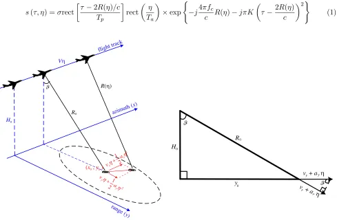
In this section, we briefly introduce the signal model for the received echo of a moving target. Figure 1 shows the geometry of a SAR in observation of a ground moving target. The moving target is modeled as a point target. We use the linear frequency modulated (LFM) signal as the transmitted signal and the baseband echo can be expressed as
s(τ, η) =σrect
τ −2R(η)/c
Tp rect η Ta ×exp
−j4πfc
c R(η)−jπK
τ− 2Rc(η)
2 (1) 2 1 2 y y v a η η + 2 1 2 x x v a η η + 0 H Vη 0 ϑ
(x , y )
R(η)
R flight track azimuth ( x) range ( y) 0 0
Figure 1. SAR geometry in observation of a ground moving target.
0 H 0 ϑ R 0 y ϑ
v y+ a yη
v + a η r
r
Figure 2. Schematic relationship betweenvrand
whereσdenotes the backscattering coefficient of the target, andτ andηare the range-time and azimuth-time, respectively. R(η) is the instantaneous slant range between the SAR and the target. Tp,fc andK denote the LFM signal’s time duration, carrier frequency and slope, respectively. Ta denotes the target exposure time in azimuth.
According to Figure 1,R(η) can be expressed as follows:
R(η) =
V η−x0−vxη− 1 2axη
2
2 +
y0+vyη+ 1 2ayη
2
2 +H2
0 (2)
In Figure 1, V and H0 denote the velocity and height of SAR platform, respectively. ϑ denotes the incident angle of SAR. (x0, y0) denotes the moving target position in the scene at η = 0. vx and
ax denote the target’s along-track velocity and acceleration, respectively. vy and ay denote the target’s across-track velocity and acceleration, respectively. We define the signs of vx and ax as positive when the target moves in the same direction as the SAR platform, otherwise as negative, whereas the signs of vy and ay as positive when the target moves far away from the track of SAR platform, otherwise is negative.
We conduct matched filtering [1] on the baseband echo signal, and the output in (τ, η) domain is expressed as follows:
s1(τ, η) =σ·Tp·sinc
τ −2Rc(η)
exp −j4πfc
c R(η)
(3)
The Doppler centroid determines the target’s azimuth position in SAR image, and the Doppler rate determines the focus degree of its image, which are two most important parameters in SAR processing. The moving target’s Doppler centroidfdc mand Doppler rateKd mare respectively expressed as follows:
fdc m = − 2R(0)
λ =−
2
λ
x0(vx−V) +y0vy
R0
(4)
Kd m = −
2R(0)
λ =−
2
λ
(vx−V)2+vy2+axx0+ayy0
R0 −
[x0(vx−V) +y0vy]2
R3 0
(5)
In (4)–(5), λ denotes the wavelength of the transmitted signal. On the other hand, for a stationary target locating at (x0, y0), its Doppler centroid fdc s and Doppler rate Kd s are expressed as follows, respectively.
fdc s = 2x0V
λR0
(6)
Kd s = − 2V2
λR0
(7)
From (4)–(7) we observe that due to the influence of motion, the moving target’s Doppler centroid and Doppler rate are different from that of stationary targets. In the following Section 3, we will analyze the influence of Doppler centroid on the moving target’s azimuth shift in SAR image.
3. THEORETICAL ANALYSIS ON THE AZIMUTH SHIFT OF A MOVING TARGET IN SAR IMAGE
In SAR imaging processing, we use the stationary target’s Doppler rate Kd s to process the moving target the azimuth position of the moving target in SAR image is then as follows:
ˆ
x0= λR0
2V fdc m=x0
1−vx
V
−y0vy
V (8)
At this moment, the offset of the moving target’s imaging position from its true position is expressed as follows:
Δˆx= ˆx0−x0=−x 0vx
V − y0vy
Since SAR imaging processing is in the slant-range plane, we use vr to denote the projection of
vy in the slant-range plane. The relationship between vr and vy is shown in Figure 2, which can be expressed as
y0
R0 = vr
vy = ar
ay
= sinϑ (10)
For the convenience of analysis, we assume that x0 = 0 in the following description. Then, the moving target’s Doppler centroid can be expressed as
fdc m=− 2vr
λ (11)
and its azimuth shift in SAR image can be expressed as
Δx=−vrR0
V (12)
From (12) we can observe that the azimuth shift is proportional tovr. In general, one can relocate the moving target in SAR image according to (12) [30]. However, (12) is valid only when the Doppler ambiguity does not occur for the moving target. In many real situations, ifvr is large and the PRF is relatively small, the Doppler ambiguity will occur, and (12) will not hold any more.
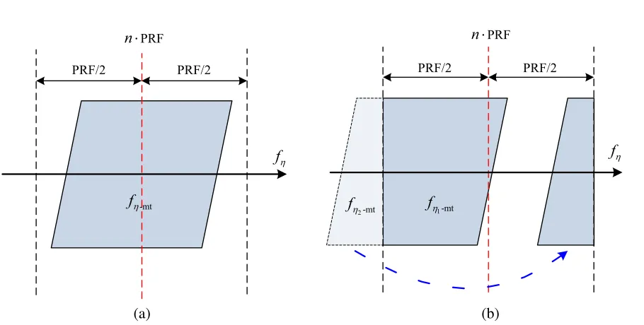
In the following, we will conduct a detailed theoretical analysis about the azimuth shift of a moving target with arbitrary velocity, no matter the Doppler ambiguity occurs nor not. Figure 3 depicts the two scenarios where the spectrum of a moving target with arbitrary velocity may situate.
Case I: entirely within a PRF band. The schematic spectrum is shown in Figure 3(a), in this
case, the target’s spectrum exists as a whole. We use fη−mt to denote the moving target’s spectrum, and it satisfies
fη−mt∈nPRF + [−PRF/2,PRF/2] (13) wheren= 0,±1,±2,±3, . . .. Ifn= 0, it means that the Doppler ambiguity does not occur.
Case II: spans in two neighboring PRF bands. The schematic spectrum is shown in
Figure 3(b), in this case, the target’s spectrum is split into two parts, which are denoted by fη1−mt and fη2−mt, respectively, and satisfy
fη1−mt ∈nPRF + [−PRF/2,PRF/2]
fη2−mt ∈(n−1)·PRF + [−PRF/2,PRF/2] (14)
fη
PRF/2
PRF
n⋅
fη
PRF
n⋅
-mt
fη fη2-mt fη1-mt
(a) (b)
PRF/2 PRF/2 PRF/2
wheren= 0,±1,±2,±3, . . ..
The processable Doppler spectrum range for SAR is [−PRF/2,PRF/2], i.e., the unambiguous range for the Doppler centroid fdc m is [−PRF/2, PRF/2]. Then, we can define the unambiguous range for
vr as follows:
vr∈[−vr prf, vr prf] (15)
wherevr prf =λ·PRF/4, and the azimuth shift corresponding tovr prf is
Δxprf =−vr prfR0
V (16)
At this moment,vr can be expressed as
vr=vr b+n·vr prf (17)
where n = fix(vr/vr prf) is called the ambiguity number, fix(·) denotes the operation of taking a value to the integer towards zero, e.g., fix(−1.9) = −1, fix(2.5) = 2. Meanwhile, we can obtain
vr b∈[−vr prf, vr prf], and the azimuth shift corresponding tovr b is
Δxb =−vr bR0
V (18)
In the following, we will use Δxb and Δxprf to represent the azimuth shift of a moving target corresponding to the above two scenarios.
Case I:entirely within a PRF band.
In this case, the moving target’s Doppler spectrum keeps as a whole. No matter how largevris, the azimuth shift is always within [−|Δxprf|,|Δxprf|]. In the following, we will analyze the two situations wheren is even andnis odd, respectively.
(1)nis even
It can be written asn= 2k (k=±0,±1,±2, . . .), andvr =vr b+ 2k·vr prf. The moving target’s Doppler centroid can be expressed as
fdc m=−
2 (vr b+ 2k·vr prf)
λ =−
2vr b
λ −k·PRF (19)
Sincek·PRF has not any effect on SAR imaging processing, it can be ignored. Then, we obtain
fdc0m =− 2vr b
λ (20)
At this moment, the moving target’s Doppler spectrum entirely locates in [−PRF/2,PRF/2]. The moving target image’s azimuth shift is
Δˆx= λR0
2V fdc0m= Δxr b (21)
(2)nis odd
If n > 0, it can be expressed as n = 2k + 1 (k = 0,1,2, . . .). At present, we have vr =
vr b + (2k+ 1)·vr prf, as well as vr b ≥ 0. The moving target’s Doppler centroid can be expressed as
fdc m=−
2 [vr b+ (2k+ 1)·vr prf]
λ =−
2vr b
λ −
PRF
2 −k·PRF (22)
After removing the k·PRF term, we obtain
fdc−1m =− 2vr b
λ −
PRF
2 (23)
Since vr b ≥ 0, we can conclude that fdc−1m ∈ [−3PRF/2,−PRF/2], i.e., the moving target’s Doppler spectrum entirely locates in [−3PRF/2, −PRF/2]. In SAR imaging processing, the spectrum will be right-shifted for PRF and locate in [−PRF/2,PRF/2], then the corresponding Doppler centroid changes to
fdc0m =fdc−1m+ PRF =− 2vr b
λ +
PRF
The moving target image’s azimuth shift is
Δˆx= λR0
2V fdc0m =
λR0 2V
−2vr b
λ +
PRF 2
= Δxr b+|Δxprf| (25)
If n < 0, it can be written as n = −(2k+ 1) (k = 0,1,2, . . .). At present, we can obtain
vr = vr b −(2k+ 1)·vr prf, and at the same time vr b ≤ 0. The moving target’s Doppler centroid can be expressed as
fdc m=− 2vr
λ =−
2 [vr b−(2k+ 1)·vr prf]
λ =−
2vr b
λ +
PRF
2 +k·PRF (26)
We remove thek·PRF term as before, and obtain
fdc1m=− 2vr b
λ +
PRF
2 (27)
Sincevr b ≤0, we can conclude thatfdc1m ∈[PRF/2,3PRF/2], i.e., the target’s Doppler spectrum entirely locates in [PRF/2,3PRF/2]. In SAR imaging processing, the spectrum will be left-shifted for PRF and locate in [−PRF/2,PRF/2], then the corresponding Doppler centroid changes to
fdc0m =fdc1m−PRF =− 2vr b
λ −
PRF
2 (28)
The azimuth shift of the moving target in SAR image is
Δˆx= λR0
2V fdc0m =
λR0 2V
−2vr b
λ −
PRF 2
= Δxr b− |Δxprf| (29)
Case II: spans in two neighboring PRF bands.
In this case, the moving target’s Doppler spectrum is split into two parts, which respectively correspond to two images in the SAR image. As same as above, in the following we will analyze the two situations, i.e., nis even and nis odd, respectively.
(1)nis even
If n≥ 0, it can be expressed as n = 2k (k = 0,1,2, . . .). At this moment, vr =vr b+ 2k·vr prf, and at the same time, vr b≥0. The moving target’s Doppler centroid can be expressed as
fdc m=− 2vr
λ =−
2 (vr b+ 2k·vr prf)
λ =−
2vr b
λ −k·PRF (30)
Thek·PRF term is removed as above. Sincevr b ≥0, the moving target’s Doppler spectrum spans in the following two neighboring PRF bands: [−PRF/2,PRF/2] and [−3PRF/2,−PRF/2].
The Doppler centroid for the spectrum part in [−PRF/2,PRF/2] is
fdc0m =− 2vr b
λ (31)
The azimuth shift of the moving target’s image corresponding to this spectrum part is
Δˆx0= λR0
2V fdc0m = Δxr b (32)
In SAR imaging processing, the spectrum part in [−3PRF/2,−PRF/2] will be right-shifted for PRF and locate in [−PRF/2,PRF/2], then the corresponding Doppler centroid becomes
fdc1m =fdc0m+ PRF =− 2vr b
λ + PRF (33)
The azimuth shift of the moving target’s image corresponding to this spectrum part is
Δˆx−1= λR0
2V fdc1m=
λR0 2V ·
−2vr b
λ + PRF
= Δxr b+ 2|Δxprf| (34)
If n < 0, it can be expressed as n = −2k (k = 1,2,3, . . .). Right now, we can obtain
vr=vr b+ 2k·vr prf and vr b≤0. The moving target’s Doppler centroid can be expressed as
fdc m=− 2vr
λ =−
2 (vr b−2k·vr prf)
λ =−
2vr b
After taking the k ·PRF term away, and since vr b ≤ 0, we can conclude that the moving target’s Doppler spectrum spans in the following two neighboring PRF bands: [−PRF/2, PRF/2] and [PRF/2,3PRF/2], respectively.
The Doppler centroid for the spectrum part in [−PRF/2,PRF/2] is
fdc0m =− 2vr b
λ (36)
The azimuth shift of the moving target’s image corresponding to this spectrum part is
Δˆx0= λR0
2V fdc0m = Δxr b (37)
In SAR imaging processing, the spectrum part in [PRF/2,3PRF/2] will be left-shifted for PRF and locate in [−PRF/2,PRF/2], then the Doppler centroid of this spectrum part changes to
fdc1m=fdc0m−PRF =− 2vr b
λ −PRF (38)
And the azimuth shift of the moving target’s image corresponding to this spectrum part is
Δˆx1 = λR0
2V fdc1m=
λR0 2V ·
−2vr b
λ −PRF
= Δxr b−2|Δxprf| (39)
(2)nis odd
If n > 0, it can be expressed as n = 2k + 1 (k = 0,1,2, . . .). At present, we have vr =
vr b+ (2k+ 1)·vr prf, and meanwhilevr b ≥0. The moving target’s Doppler centroid can be expressed as
fdc m=−
2 [vr b+ (2k+ 1)·vr prf]
λ =−
2vr b
λ −
PRF
2 −k·PRF (40)
After taking thek·PRF term away, and sincevr b ≥0, the moving target’s Doppler spectrum spans in the following two neighboring PRF bands: [−PRF/2, PRF/2] and [−3PRF/2,−PRF/2], respectively.
The Doppler centroid for the spectrum part in [−PRF/2,PRF/2] is
fdc0m=− 2vr b
λ −
PRF
2 (41)
And the azimuth shift of the moving target’s image corresponding to this spectrum part is
Δˆx0 = Δxr b− |Δxprf| (42)
The spectrum part in [−3PRF/2,−PRF/2] will be right-shifted for PRF and locate in [−PRF/2,PRF/2] in SAR imaging processing, then the corresponding Doppler centroid changes to
fdc1m =fdc0m+ PRF =− 2vr b
λ +
PRF
2 (43)
And the azimuth shift of the moving target’s image corresponding to this spectrum part is
Δˆx−1 = Δxr b+|Δxprf| (44)
If n < 0, it can be expressed as n = −(2k+ 1) (k = 0,1,2, . . .). Now, we can obtain
vr=vr b−(2k+ 1)·vr prf and vr b≤0. The Doppler centroid for the moving target is
fdc m=− 2vr
λ =−
2 [vr b−(2k+ 1)·vr prf]
λ =−
2vr b
λ +
PRF
2 +k·PRF (45)
After taking away thek·PRF term, and sincevr b≤0, the target’s Doppler spectrum spans in the following two neighboring PRF bands: [−PRF/2,PRF/2], respectively.
The Doppler centroid for the spectrum part in [PRF/2,3PRF/2] is
fdc0m=− 2vr b
λ +
PRF
2 (46)
The azimuth shift of the moving target’s image corresponding to this spectrum part is
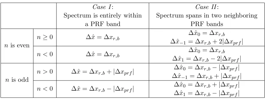
Table 1. Summarization of the moving target’s azimuth shift for the two scenarios.
Case I:
Spectrum is entirely within a PRF band
Case II:
Spectrum spans in two neighboring PRF bands
nis even
n≥0 Δˆx= Δxr b Δˆx0= Δxr b Δˆx−1 = Δxr b+ 2|Δxprf|
n <0 Δˆx= Δxr b Δˆx0= Δxr b Δˆx1 = Δxr b−2|Δxprf|
nis odd
n >0 Δˆx= Δxr b+|Δxprf| Δˆx0 = Δxr b− |Δxprf| Δˆx−1 = Δxr b+|Δxprf|
n <0 Δˆx= Δxr b− |Δxprf| Δˆx0 = Δxr b+|Δxprf| Δˆx1 = Δxr b− |Δxprf|
The spectrum part in [PRF/2,3PRF/2] will be left-shifted for PRF and locate in [−PRF/2, PRF/2] in SAR imaging processing, then the Doppler centroid for this spectrum part changes to
fdc1m =fdc0m−PRF =− 2vr b
λ −
PRF
2 (48)
The corresponding azimuth shift of the moving target’s image is
Δˆx1 = Δxr b− |Δxprf| (49)
We summarize above analysis results in Table 1. According to these formulas, we can relocate a moving target with arbitrary velocity to its correct azimuthal position in SAR image after estimating its velocity.
4. SIMULATION
In this section, we conduct simulations to validate the analysis in Section 3. The simulated system parameters are listed in Table 2. In the simulations, we utilize the range-Doppler algorithm [1] for imaging processing.
According to the SAR system parameters in Table 2, we calculate that vr prf = 6 m/s, and |Δxprf|= 195.16 m. Suppose the moving target locates at the scene center whenη= 0, i.e.,x0 = 0. At this moment, the SAR incident angle on target isϑ= 45◦. We ignore the target’s range cell migration (RCM), and assume its across-track acceleration, along-track velocity and along-track acceleration are all zeros, i.e., ay = 0 m/s2,vx = 0 m/s,ax= 0 m/s2.
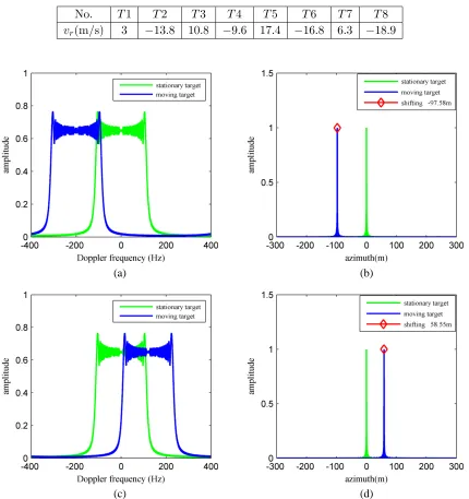
In the following, we will simulate the imaging of moving targets with different velocities in the situations discussed in Section 3. The velocities of the moving targets are listed in Table 3.
(1)T1 andT2 are inCase I and nis even.
We can calculate thatn= 0, vr b = 3 m/s for T1. According to Table 2, the azimuth shift ofT1 is calculated as Δˆx0 =−97.58 m, and the simulated results are shown in Figures 4(a) and (b), respectively.
Table 2. Simulated SAR system parameters.
carrier frequencyfc 10.0 GHz azimuth beamwidth 2◦
bandwidthB 50 MHz PRF 800
pulse durationTp 5µs platform velocity V 100 m/s range sampling rate Fs 75 MHz platform heightH0 2300 m
Whereas forT2,n=−2,vr b=−1.8 m/s, the azimuth shift ofT2 is calculated as Δˆx0 = 58.55 m, and the simulated results are shown in Figures 4(c) and (d), respectively. From Figure 4 we can observe that the Doppler spectra of both T1 and T2 keep as a whole, and the simulated azimuth shifts agree with the theoretic values very well. In Figure 4 and the following figures, the Doppler spectrum and the azimuth profile of a stationary target are also plotted for reference.
(2)T3 andT4 are inCase I and nis odd.
ForT3, we can obtain thatn= 1, vr b= 4.8 m/s, according to Table 2, the azimuth shift of T3 is calculated as Δˆx0= 39.03 m, and the simulated results are shown in Figures 5(a) and (b), respectively.
Table 3. Simulated moving targets’ velocities.
No. T1 T2 T3 T4 T5 T6 T7 T8
vr(m/s) 3 −13.8 10.8 −9.6 17.4 −16.8 6.3 −18.9
(a) (b)
(c) (d)
(a) (b)
(c) (d)
Figure 5. Simulation results for Case I: the target’s spectrum is entirely within a PRF band and n is odd. (a) Doppler spectrum of T3 (vr = 10.8 m/s), (b) azimuth profile of T3 (vr = 10.8 m/s), (c) Doppler spectrum of T4 (vr =−9.6 m/s), (d) azimuth profile of T4 (vr=−9.6 m/s).
Whereas forT4,n=−1 andvr b=−3.6 m/s, according to Table 2, the azimuth shift ofT4 is calculated as Δˆx0 = −78.06 m and the simulated results are shown in Figures 5(c) and (d), respectively. From Figure 5, we can see that the Doppler spectra of T3 and T4 also keep as a whole, and the simulated results agree with the theoretic results very well.
(3)T5 andT6 are inCase II and nis even.
We calculate thatn= 2, vr b = 5.4 m/s forT5. According to Table 2, the azimuth shifts for T5’s two images are calculated as Δˆx0 = −175.65 m and Δˆx−1 = 214.68 m, and the simulated results are shown in Figures 6(a) and (b), respectively. Whereas forT6,n=−2 andvr b=−4.8 m/s are calculated. According to Table 2, the azimuth shifts forT6’s two images are Δˆx0= 156.13 m and Δˆx1 =−234.19 m, and the simulated results are shown in Figures 6(c) and (d), respectively. From Figure 6, we can see that the spectra of T5 and T6 are both split into two parts, and the simulated azimuth shifts agree with the theoretic values.
(4)T7 andT8 are inCase II and nis odd.
(a) (b)
(c) (d)
Figure 6. Simulation results for Case II: the target’s spectrum spans in two neighboring PRF bands, and n is even. (a) Doppler spectrum ofT5 (vr = 17.4 m/s), (b) azimuth profile of T5 (vr = 17.4 m/s), (c) Doppler spectrum ofT6 (vr=−16.8 m/s), (d) azimuth profile of T6 (vr=−16.8 m/s).
(c) (d)
Figure 7. Simulation results for Case II: the target’s spectrum spans in two neighboring PRF bands, and nis odd. (a) Doppler spectrum of T7 (vr = 6.3 m/s), (b) azimuth image of T7 (vr= 6.3 m/s), (c) Doppler spectrum of T8 (vr =−18.9 m/s), (d) azimuth image ofT8 (vr =−18.9 m/s).
T8 is vr = −18.9 m/s, at this time, n = −3 and vr b = −0.9 m/s. According to Table 2, we get Δˆx0 = −165.89 m and Δˆx1 = 224.44 m for T8, respectively. The simulation results are shown in Figures 7(c) and (d), respectively. From Figure 7 we can see that the spectra of T7 andT8 are both split into two parts, and the simulated azimuth shifts also agree with the theoretic values.
5. CONCLUSION
In this paper, we conduct a detailed theoretical analysis on the azimuth shift issue of a moving target in SAR image whose spectrum may entirely situate within a PRF band or spans in two neighboring PRF bands. The analyzed results are summarized and validated by simulations. Based on the derived analytical formulas, one can get the correct azimuth shift for a moving target with arbitrary velocity, which is beneficial for moving targets relocation in SAR image processing.
REFERENCES
1. Cumming, I. G. and F. H. Wong, Digital Signal Processing of Synthetic Aperture Radar Data:
Algorithms and Implementation, Artech House, Boston, MA, 2005.
2. Jao, J. K., “Theory of synthetic aperture radar imaging of a moving target,” IEEE Transactions
on Geoscience and Remote Sensing, Vol. 39, No. 9, 1984–1992, 2001.
3. Zhang, Y., W. Zhai, X. Zhang, X. Shi, X. Gu, and Y. Deng, “Ground moving train imaging by Ku-band radar with two receiving channels,”Progress In Electromagnetics Research, Vol. 130, 493–512, 2012.
4. Yang, J., C. Liu, and Y. F. Wang, “Imaging and parameter estimation of fast-moving targets with single-antenna SAR,”IEEE Geoscience and Remote Sensing Letters, Vol. 11, No. 2, 529–533, 2014. 5. Yang, J., C. Liu, and Y. F. Wang, “Detection and imaging of ground moving targets with real SAR
data,” IEEE Transactions on Geoscience and Remote Sensing, Vol. 53, No. 2, 920–932, 2015. 6. Mao, X., D.-Y. Zhu, and Z.-D. Zhu, “Signatures of moving target in polar format spotlight SAR
image,” Progress In Electromagnetics Research, Vol. 92, 47–64, 2009.
8. Chiu, S. and C. Livingstone, “A comparison of displaced phase centre antenna and along-track interferometry techniques for RADARSAT-2 ground moving target indication,” Canadian Journal
of Remote Sensing, Vol. 31, 37–51, 2005.
9. Cerutti-Maori, D. and I. Sikaneta, “A generalization of DPCA processing for multichannel SAR/GMTI radars,”IEEE Transactions on Geoscience and Remote Sensing, Vol. 51, No. 1, 560– 572, 2013.
10. Moccia, A. and G. Rufino, “Spaceborne along-track SAR interferometry: Performance analysis and mission scenarios,” IEEE Transactions on Aerospace and Electronic Systems, Vol. 37, No. 1, 199–213, 2001.
11. Romeiser, R., H. Breit, M. Eineder, and H. Runge, “Demonstration of current measurements from space by along-track SAR interferometry with SRTM data,” 2002 IEEE International Geoscience
and Remote Sensing Symposium, 2002.
12. Budillon, A., A. Evangelista, and G. Schirinzi, “GLRT detection of moving targets via multibaseline along-track interferometric SAR systems,” IEEE Geoscience and Remote Sensing Letters, Vol. 9, No. 3, 348–352, 2012.
13. Tian, B., D.-Y. Zhu, and Z.-D. Zhu, “A novel moving target detection approach for dual-channel SAR system,” Progress In Electromagnetics Research, Vol. 115, 191–206, 2011.
14. Dipietro, R. C., “Extended factor space-time processing for airborne radar system,”The
Twenty-Sixth Asilomar Conference on Signals, Systems and Computers, 1992.
15. Chen, H. C. and C. D. McGillem, “Target motion compensation by spectrum shifting in synthetic aperture radar,”IEEE Transactions on Aerospace and Electronic Systems, Vol. 28, No. 3, 895–901, 1992.
16. Moreira, J. R. and W. Keydel, “A new MTI-SAR approach using the reflectivity displacement method,”IEEE Transactions on Geoscience and Remote Sensing, Vol. 33, No. 5, 1238–1244, 1995. 17. Lv, G., J. Wang, and X. Liu, “Ground moving target indication in SAR images by symmetric
defocusing,” IEEE Geoscience and Remote Sensing Letters, Vol. 10, No. 2, 241–245, 2013.
18. Perry, R. P., R. C. DiPietro, and R. L. Fante, “SAR imaging of moving targets,”IEEE Transactions
on Aerospace and Electronic Systems, Vol. 35, No. 1, 188–200, 1999.
19. Zhou, F., R. Wu, M. Xing, and Z. Bao, “Approach for single channel SAR ground moving target imaging and motion parameter estimation,”IET Radar Sonar and Navigation, Vol. 1, No. 1, 59–66, 2007.
20. Zhu, D., Y. Li, and Z. Zhu, “A keystone transform without interpolation for SAR ground moving-target imaging,” IEEE Geoscience and Remote Sensing Letters, Vol. 4, No. 1, 18–22, 2007.
21. Li, G., X. G. Xia, and Y. N. Peng, “Doppler keystone transform: an approach suitable for parallel implementation of SAR moving target imaging,” IEEE Geoscience and Remote Sensing Letters, Vol. 5, No. 4, 573–577, 2008.
22. Yang, J. F. and Y. H. Zhang, “Novel compressive sensing-based Dechirp-Keystone algorithm for synthetic aperture radar imaging of moving target,” IET Radar Sonar and Navigation, Vol. 9, No. 5, 509–518, 2015.
23. Yang, J. and Y. Zhang, “A novel Keystone transform based algorithm for moving target imaging with Radon transform and fractional Fourier transform involved,” PIERS Proceedings, 1406–1410, Guangzhou, Aug. 25–28, 2014.
24. Kong, Y. K., B. L. Cho, and Y. S. Kim, “Ambiguity-free Doppler centroid estimation technique for airborne SAR using the Radon transform,”IEEE Transactions on Geoscience and Remote Sensing, Vol. 43, No. 4, 715–721, 2005.
25. Cumming, I. G. and S. Li, “Improved slope estimation for SAR Doppler ambiguity resolution,”
IEEE Transactions on Geoscience and Remote Sensing, Vol. 44, No. 3, 707–718, 2006.
26. Zhu, S., G. Liao, B. Liu, and Y. Qu, “New approach for SAR Doppler ambiguity resolution in compressed range time and scaled azimuth time domain,” IEEE Transactions on Aerospace and
27. Barbarossa, S. and A. Farina, “Detection and imaging of moving objects with synthetic aperture radar. Part 2: Joint time-frequency analysis by Wigner-Ville distribution,”IEE Radar and Signal
Processing, 89–97, 1992.
28. Sun, H., G. S. Liu, H. Gu, and W. M. Su, “Application of the fractional Fourier transform to moving target detection in airborne SAR,” IEEE Transactions on Aerospace and Electronic
Systems, Vol. 38, No. 4, 1416–1424, 2002.
29. Djurovic, I., T. Thayaparan, and L. J. Stankovic, “SAR imaging of moving targets using polynomial Fourier transform,” IET Signal Processing, Vol. 2, 237–246, 2008.
30. Zhang, X. P., G. S. Liao, S. Q. Zhu, C. Zeng, and Y. X. Shu, “Geometry-information-aided efficient radial velocity estimation for moving target imaging and location based on Radon transform,”IEEE
Transactions on Geoscience and Remote Sensing, Vol. 53, No. 2, 1105–1117, 2015.
31. Zhu, S. Q., G. S. Liao, Y. Qu, Z. G. Zhou, and X. Y. Liu, “Ground moving targets imaging algorithm for synthetic aperture radar,” IEEE Transactions on Geoscience and Remote Sensing, Vol. 49, No. 1, 462–477, 2011.